florida public hurricane loss model 5.0 - Florida State Board of ...
florida public hurricane loss model 5.0 - Florida State Board of ...
florida public hurricane loss model 5.0 - Florida State Board of ...

Create successful ePaper yourself
Turn your PDF publications into a flip-book with our unique Google optimized e-Paper software.
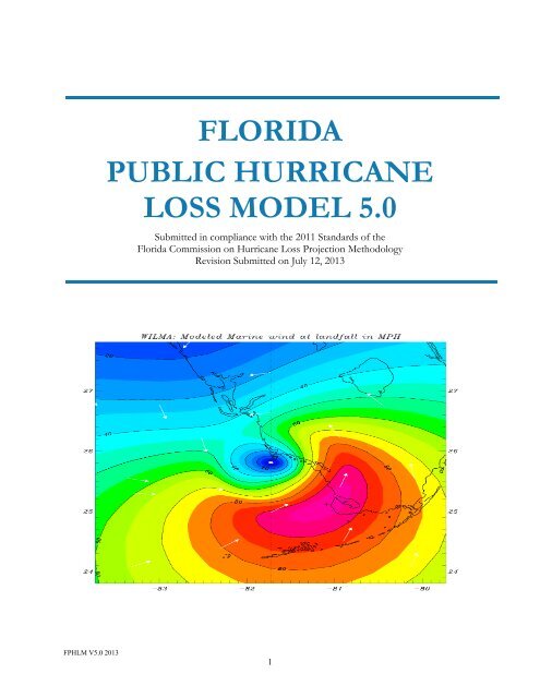
FLORIDAPUBLIC HURRICANELOSS MODEL <strong>5.0</strong>Submitted in compliance with the 2011 Standards <strong>of</strong> the<strong>Florida</strong> Commission on Hurricane Loss Projection MethodologyRevision Submitted on July 12, 2013FPHLM V<strong>5.0</strong> 20131
Model IdentificationName <strong>of</strong> Model and Version: <strong>Florida</strong> Public Hurricane Loss Model <strong>5.0</strong>Name <strong>of</strong> Modeling Organization: <strong>Florida</strong> International UniversityStreet Address: International Hurricane Research Center, MARC 360City, <strong>State</strong>, ZIP Code: Miami, <strong>Florida</strong> 33199Mailing Address, if different from above: Same as aboveContact Person: Shahid S. HamidPhone Number: 305-348-2727 Fax: 305-348-1761E-mail Address: hamids@fiu.eduDate: July 12, 2013FPHLM V<strong>5.0</strong> 20132
July 12, 2013Chair, <strong>Florida</strong> Commission on Hurricane Loss Projection Methodologyc/o Donna Sirmons<strong>Florida</strong> <strong>State</strong> <strong>Board</strong> <strong>of</strong> Administration1801 Hermitage Boulevard, Suite 100Tallahassee, FL 32308Dear Commission Chairman:I am pleased to inform you that the final version <strong>of</strong> <strong>5.0</strong> <strong>of</strong> <strong>Florida</strong> Public Hurricane Loss Modelis ready for review by the Commission. The FPHLM <strong>model</strong> has been reviewed by pr<strong>of</strong>essionalshaving credentials and/or experience in the areas <strong>of</strong> meteorology, engineering, actuarial science,statistics and computer science; for compliance with the Standards, as documented by the expertcertification forms G1-G7.Enclosed are 7 bound copies <strong>of</strong> our submission, which includes the summary statement <strong>of</strong>compliance with the standards, the forms, and the submission checklist.Please contact me if you have any questions regarding this submission.Sincerely,Shahid Hamid, Ph.D., CFAPr<strong>of</strong>essor <strong>of</strong> Finance, andDirector, Laboratory for Insurance, Economic and Financial ResearchInternational Hurricane Research CenterRB 202B, Department <strong>of</strong> Finance, College <strong>of</strong> Business<strong>Florida</strong> International UniversityMiami, FL 33199tel: 305 348 2727 fax: 305 348 4245Cc: Kevin M. McCarty, Insurance CommissionerFPHLM V<strong>5.0</strong> 20133
<strong>State</strong>ment <strong>of</strong> Compliance and Trade Secret DisclosureItemsThe <strong>Florida</strong> Public Hurricane Loss Model v<strong>5.0</strong> is intended to comply with each Standard <strong>of</strong> the2011 Report <strong>of</strong> Activities released by the <strong>Florida</strong> Commission on Hurricane Loss ProjectionMethodology. The required disclosures, forms, and analysis are contained herein.The source code for the <strong>loss</strong> <strong>model</strong> will be available for review by the Pr<strong>of</strong>essional Team.FPHLM V<strong>5.0</strong> 20134
Model Submission Checklist1. Please indicate by checking below that the foll owing has been include d in your subm issiondocumentation to the <strong>Florida</strong> Commission on Hurricane Loss Projection Methodology.Yes No ItemX 1. Letter to the Commissiona. Refers to the certification forms and s tates that pr<strong>of</strong>essionals ha ving credentialsand/or experience in the areas <strong>of</strong> meteorology, engineering, actuarial science,statistics, and computer science have reviewed the <strong>model</strong> for compliance with theXstandardsXb. <strong>State</strong>s <strong>model</strong> is ready to be reviewed by the Pr<strong>of</strong>essional TeamXc. Any caveats to the above statements noted with a complete explanation2. Summary state ment <strong>of</strong> co mpliance with each individual standard and the data andXanalyses required in the disclosures and forms3. General description <strong>of</strong> any trade secret information the <strong>model</strong>ing organization intendsXto present to the Pr<strong>of</strong>essional TeamX 4. Model IdentificationX 5. Seven (7) Bound Copies (duplexed)X 6. Link containing:Xa. Submission text in PDF formatXb. PDF file highlightable and bookmarked by standard, form, and sectionc. Data file names include abbreviated name <strong>of</strong> m odeling organization, standardsXyear, and form name (when applicable)Xd. Form S-6 (if required) in ASCII and PDF formatXe. Forms M-1, M-3, V-2, A-1, A-2, A-3, A-4, A-5, A-7, and A-8 in Excel formatX 7. Table <strong>of</strong> Contents8. Materials consecutively numbered from beginning to end starting with the first pageX(including cover) using a single numbering system9. All tables, graphs, and o ther non-text items consecutively num bered using wholeXnumbersX 10. All tables, graphs, and other non-text items specifically listed in Table <strong>of</strong> ContentsX 11. All tables, graphs, and other non-text items clearly labeled with abbreviations defined12. All column headings shown and repeated at the top <strong>of</strong> every subsequent page for formsXand tables13. Standards, disclosures, and forms in italics, <strong>model</strong>ing organization responses in nonitalicsXX 14. Graphs accompanied by legends and labels for all elementsX 15. All units <strong>of</strong> measurement clearly identified with appropriate units used16. Hard copy <strong>of</strong> all forms included in a submission document Appendix exceptXForms V-3, A-6, and S-6FPHLM V<strong>5.0</strong> 20135
2. Explanation <strong>of</strong> “No” responses indicated above. (Attach additional pages if needed.)<strong>Florida</strong> Public Hurricane LossModel <strong>5.0</strong>July 12, 2013Model Name Modeler Signature DateFPHLM V<strong>5.0</strong> 20136
Table <strong>of</strong> ContentsGENERAL STANDARDS ......................................................................................................... 16G-1 Scope <strong>of</strong> the Computer Model and Its Implementation ................................................. 16G-2 Qualifications <strong>of</strong> Modeling Organization Personnel and Consultants ......................... 117G-3 Risk Location ............................................................................................................... 125G-4 Independence <strong>of</strong> Model Components ........................................................................... 127G-5 Editorial Compliance .................................................................................................... 128Form G-1 ................................................................................................................................. 129Form G-2 ................................................................................................................................. 130Form G-3 ................................................................................................................................. 131Form G-4 ................................................................................................................................. 132Form G-5 ................................................................................................................................. 133Form G-6 ................................................................................................................................. 134Form G-7 ................................................................................................................................. 135METEOROLOGICAL STANDARDS .................................................................................... 136M-1 Base Hurricane Storm Set ............................................................................................ 136M-2 Hurricane Parameters and Characteristics .................................................................... 138M-3 Hurricane Probabilities ................................................................................................. 146M-4 Hurricane Windfield Structure ..................................................................................... 148M-5 Landfall and Over-Land Weakening Methodologies ................................................... 156M-6 Logical Relationships <strong>of</strong> Hurricane Characteristics ..................................................... 161Form M-1: Annual Occurrence Rates ..................................................................................... 163Form M-2: Maps <strong>of</strong> Maximum Winds ................................................................................... 168Form M-3: Radius <strong>of</strong> Maximum Winds and Radii <strong>of</strong> Standard Wind Thresholds ................. 174VULNERABILITY STANDARDS ........................................................................................... 179V-1 Derivation <strong>of</strong> Vulnerability Functions ......................................................................... 179V-2 Derivation <strong>of</strong> Contents and Time Element Vulnerability Functions ............................ 237V-3 Mitigation Measures ..................................................................................................... 241Form V-1: One Hypothetical Event ........................................................................................ 245Form V-2: Mitigation Measures – Range <strong>of</strong> Changes in Damage ......................................... 252Form V-3: Mitigation Measures – Mean Damage Ratio ........................................................ 255ACTUARIAL STANDARDS ................................................................................................... 266A-1 Modeling Input Data .................................................................................................... 266A-2 Event Definition ........................................................................................................... 275A-3 Modeled Loss Cost and Probable Maximum Loss Considerations .............................. 276A-4 Policy Conditions ......................................................................................................... 280A-5 Coverages ..................................................................................................................... 283A-6 Loss Output .................................................................................................................. 286Form A-1: Zero Deductible Personal Residential Loss Costs by ZIP Code ........................... 290Form A-2: Base Hurricane Storm Set <strong>State</strong>wide Loss Costs .................................................. 294Form A-3: Cumulative Losses from the 2004 Hurricane Season ........................................... 295FPHLM V<strong>5.0</strong> 20137
Form A-4: Output Ranges ....................................................................................................... 301Form A-5: Percentage Change in Output Ranges ................................................................... 302Form A-6: Personal Residential Output Ranges ..................................................................... 311Form A-7: Percentage Change in Logical Relationship to Risk ............................................. 312Form A-8: Probable Maximum Loss for <strong>Florida</strong> .................................................................... 312STATISTICAL STANDARDS ................................................................................................. 316S-1 Modeled Results and Goodness-<strong>of</strong>-Fit ......................................................................... 316S-2 Sensitivity Analysis for Model Output......................................................................... 328S-3 Uncertainty Analysis for Model Output ....................................................................... 331S-4 County Level Aggregation ........................................................................................... 334S-5 Replication <strong>of</strong> Known Hurricane Losses ..................................................................... 335S-6 Comparison <strong>of</strong> Projected Hurricane Loss Costs .......................................................... 339Form S-1: Probability and Frequency <strong>of</strong> <strong>Florida</strong> Landfalling Hurricanes per Year .............. 340Form S-2: Examples <strong>of</strong> Loss Exceedance Estimates ............................................................. 341Form S-3: Distributions <strong>of</strong> Stochastic Hurricane Parameters ................................................ 342Form S-4: Validation Comparisons ....................................................................................... 343Form S-5: Average Annual Zero Deductible <strong>State</strong>wide Loss Costs – Historical versusModeled .................................................................................................................................. 349Form S-6: Hypothetical Events for Sensitivity and Uncertainty Analysis ............................ 351COMPUTER STANDARDS .................................................................................................... 358C-1 Documentation ............................................................................................................. 358C-2 Requirements ................................................................................................................ 360C-3 Model Architecture and Component Design ................................................................ 361C-4 Implementation............................................................................................................. 362C-5 Verification ................................................................................................................... 364C-6 Model Maintenance and Revision ................................................................................ 367C-7 Security ......................................................................................................................... 370Appendix A – Expert Review Letters ..................................................................................... 371Appendix B – Form A-2: Base Hurricane Storm Set <strong>State</strong>wide Loss Costs .......................... 379Appendix C – Form A-3: Cumulative Losses from the 2004 Hurricane Season ................... 382Appendix D – Form A-4: Output Ranges ............................................................................... 399Appendix E – Form A-5: Percentage Change in Output Ranges ........................................... 420Appendix F – Form A-6: Logical Relationship to Risk .......................................................... 422Appendix G – Form A-7: Percentage Change in Logical Relationship to Risk ..................... 467Appendix H – Form A-8: Probable Maximum Loss for <strong>Florida</strong> ............................................ 476FPHLM V<strong>5.0</strong> 20138
List <strong>of</strong> FiguresFIGURE 1. PROCESS TO ASSURE CONTINUAL AGREEMENT AND CORRECT CORRESPONDENCE. ........ 17FIGURE 2. FLORIDA PUBLIC HURRICANE LOSS MODEL DOMAIN. CIRCLES REPRESENT THE THREATZONE. BLUE COLOR INDICATES WATER DEPTH EXCEEDING 656 FT (200 M). .......................... 19FIGURE 3. EXAMPLES OF SIMULATED HURRICANE TRACKS. NUMBERS REFER TO THE STOCHASTICTRACK NUMBER, AND COLORS REPRESENT STORM INTENSITY BASED ON CENTRAL PRESSURE.DASHED LINES REPRESENT TROPICAL STORM STRENGTH WINDS, AND CAT 1-5 WINDS AREREPRESENTED BY BLACK, BLUE, ORANGE, RED, AND TURQUOISE, RESPECTIVELY................... 21FIGURE 4. COMPARISON BETWEEN THE MODELED AND OBSERVED WILLOUGHBY AND RAHN (2004)B DATASET. ............................................................................................................................ 22FIGURE 5. OBSERVED AND EXPECTED DISTRIBUTION FOR RMAX. THE X-AXIS IS THE RADIUS INSTATUTE MILES, AND THE Y-AXIS IS THE FREQUENCY OF OCCURRENCE. ................................. 23FIGURE 6. COMPARISON OF 100,000 RMAX VALUES SAMPLED FROM THE GAMMA DISTRIBUTION FORCATEGORY 1-4 STORMS TO THE EXPECTED VALUES. .............................................................. 24FIGURE 7. TYPICAL SINGLE-FAMILY HOMES (GOOGLE EARTH). ..................................................... 27FIGURE 8. MANUFACTURED HOMES (GOOGLE EARTH). ................................................................. 28FIGURE 9. REGIONAL CLASSIFICATION OF FLORIDA WITH THE CORRESPONDING SAMPLE COUNTIES(BLUE AND STAR). .................................................................................................................. 28FIGURE 10. MONTE CARLO SIMULATION PROCEDURE TO PREDICT EXTERNAL DAMAGE. ................ 33FIGURE 11. PROCEDURE TO CREATE VULNERABILITY MATRIX. ...................................................... 37FIGURE 12. WEIGHTED MASONRY STRUCTURE VULNERABILITIES IN THE CENTRAL WIND-BORNEDEBRIS REGION. ...................................................................................................................... 41FIGURE 13. TYPICAL LOW-RISE BUILDINGS (LB)............................................................................ 49FIGURE 14. EXAMPLES OF MID- AND HIGH-RISE BUILDINGS (MHB)............................................... 49FIGURE 15. APARTMENT TYPES ACCORDING TO LAYOUT (LEFT: CLOSED BUILDING WITH INTERIORENTRY DOOR; RIGHT: OPEN BUILDING WITH EXTERIOR ENTRY DOOR). ................................... 52FIGURE 16. FLOWCHART OF THE INTERIOR DAMAGE MODEL. ......................................................... 56FIGURE 17. MEAN ACCUMULATED IMPINGING RAIN AS A FUNCTION OF PEAK 3-SECOND WIND GUST................................................................................................................................................ 61FIGURE 18. EXTERIOR AND INTERIOR DAMAGE ASSESSMENT FOR MHB. ....................................... 66FIGURE 19. FLOW DIAGRAM OF THE COMPUTER MODEL. ................................................................ 72FIGURE 20. PERSONAL RESIDENTIAL AND COMMERCIAL RESIDENTIAL COUNTY WIDE PERCENTAGECHANGE DUE TO UPDATE OF PROBABILITY DISTRIBUTION FUNCTIONS. ................................. 112FIGURE 21. PERSONAL RESIDENTIAL AND COMMERCIAL RESIDENTIAL COUNTY WIDE PERCENTAGECHANGE DUE TO UPDATE OF ZIP CODE CENTROIDS. ............................................................. 113FPHLM V<strong>5.0</strong> 20139
FIGURE 22. PERSONAL RESIDENTIAL AND COMMERCIAL RESIDENTIAL COUNTY WIDE PERCENTAGECHANGE DUE TO CHANGE IN HURRICANE PBL HEIGHT. ........................................................ 114FIGURE 23. COUNTY WIDE PERCENTAGE CHANGE DUE TO VULNERABILITY FUNCTIONS PERSONALRESIDENTIAL MODEL. ........................................................................................................... 115FIGURE 24. COUNTY WIDE PERCENTAGE CHANGE DUE TO NEW VULNERABILITY FUNCTIONSCOMMERCIAL RESIDENTIAL MODEL. ..................................................................................... 116FIGURE 25. ORGANIZATIONAL STRUCTURE. ................................................................................. 118FIGURE 26. FLORIDA PUBLIC HURRICANE LOSS MODEL WORKFLOW. ......................................... 122FIGURE 27. COMPARISON OF OBSERVED LANDFALL RMAX (SM) DISTRIBUTION TO A GAMMADISTRIBUTION FIT OF THE DATA............................................................................................ 140FIGURE 28. COMPARISON OF 100,000 RMAX VALUES SAMPLED FROM THE GAMMA DISTRIBUTIONFOR CAT 1–4 STORMS TO THE EXPECTED VALUES. ............................................................... 141FIGURE 29. ANALYSIS OF 742 GPS DROPSONDE PROFILES LAUNCHED FROM 2-4 KM WITH FLIGHT-LEVEL WINDS AT LAUNCH GREATER THAN HURRICANE FORCE AND WITH MEASURED SURFACEWINDS. UPPER FIGURE: DEPENDENCE OF THE RATIO OF 10 M WIND SPEED (U10) TO THE MEANBOUNDARY LAYER WIND SPEED (MBL) ON THE SCALED RADIUS (RATIO OF RADIUS OF LASTMEASURED WIND (RLMW) TO THE RADIUS OF MAXIMUM WIND AT FLIGHT LEVEL (RMAXFL).LOWER FIGURE: SURFACE WIND FACTOR (U10/MBL) DEPENDENCE ON MAXIMUM FLIGHTLEVEL WIND SPEED (VFLMAX, IN UNITS OF MILES PER HOUR / 2.23). .................................... 143FIGURE 30. AXISYMMETRIC ROTATIONAL WIND SPEED (MPH) VS. SCALED RADIUS FOR B = 1.38,DELP = 49.1 MB. .................................................................................................................. 149FIGURE 31. UPSTREAM FETCH WIND EXPOSURE PHOTOGRAPH FOR CHATHAM, MS (LEFT, LOOKINGNORTH), AND PANAMA CITY, FL (RIGHT, LOOKING NORTHEAST). AFTER POWELL ET AL.(2004). ................................................................................................................................. 151FIGURE 32. COMPARISON OF MODELED (LEFT) AND OBSERVED (H*WIND, RIGHT) LANDFALL WINDFIELDS OF HURRICANE CHARLEY (2004, TOP) AND HURRICANE JEANNE (2004, BOTTOM). LINESEGMENT INDICATES STORM HEADING. HORIZONTAL COORDINATES ARE IN UNITS OF R/RMAXAND WINDS UNITS OF MILES PER HOUR. ALL WIND FIELDS ARE FOR MARINE EXPOSURE. ..... 153FIGURE 33. AS IN FIG. 33 BUT FOR HURRICANE WILMA OF 2005. ................................................ 154FIGURE 34. OBSERVED (GREEN) AND MODELED (BLACK) MAXIMUM SUSTAINED SURFACE WINDS ASA FUNCTION OF TIME FOR 2004 HURRICANES FRANCES (LEFT) AND CHARLEY (RIGHT).LANDFALL IS REPRESENTED BY THE VERTICAL DASH-DOT RED LINE AT THE LEFT AND TIME OFEXIT AS THE RED LINE ON THE RIGHT. ................................................................................... 157FIGURE 35. OBSERVED (GREEN) AND MODELED (BLACK) MAXIMUM SUSTAINED SURFACE WINDS ASA FUNCTION OF TIME FOR HURRICANES JEANNE (2004, TOP LEFT), KATRINA (2005 IN SOUTHFLORIDA, TOP RIGHT), AND WILMA (2005, LOWER LEFT). LANDFALL IS REPRESENTED BY THEVERTICAL DASH-DOT RED LINE AT THE LEFT AND TIME OF EXIT AS THE RED LINE ON THE RIGHT.............................................................................................................................................. 158FIGURE 36. FORM M-1 COMPARISON OF MODELED AND HISTORICAL LANDFALLING HURRICANEFREQUENCY (STORMS OCCURRING IN 112 YEARS) FOR REGIONS A–F, FL STATEWIDEFPHLM V<strong>5.0</strong> 201310
LANDFALLS (ONE PER FL REGION), FL BYPASSING STORMS, AND FL STATE-WIDE HURRICANES.............................................................................................................................................. 166FIGURE 37. MAXIMUM ZIP CODE WIND SPEED FOR OPEN TERRAIN WIND EXPOSURE BASED ONSIMULATIONS OF THE HISTORICAL STORM SET. ..................................................................... 170FIGURE 38. MAXIMUM ZIP CODE WIND SPEED FOR ACTUAL TERRAIN WIND EXPOSURE BASED ONSIMULATIONS OF THE HISTORICAL STORM SET. ..................................................................... 171FIGURE 39. 100- AND 250-YEAR RETURN PERIOD WIND SPEEDS AT FLORIDA ZIP CODES FOR OPENTERRAIN WIND EXPOSURE. ................................................................................................... 172FIGURE 40. 100- AND 250-YEAR RETURN PERIOD WIND SPEEDS AT FLORIDA ZIP CODES FORACTUAL TERRAIN WIND EXPOSURE. ...................................................................................... 173FIGURE 41. REPRESENTATIVE SCATTER PLOT OF THE MODEL INPUT RADIUS OF MAXIMUM WIND (YAXIS) VERSUS MINIMUM SEA-LEVEL AIR PRESSURE AT LANDFALL (MB). RELATIVEHISTOGRAMS FOR EACH QUANTITY ARE ALSO SHOWN. ......................................................... 177FIGURE 42. ONE WAY BOX PLOT (LEFT) OF RMAX (CONTINUOUS) RESPONSE ACROSS 10 MB PMINGROUPS. BOXES (AND WHISKERS) ARE IN RED; STANDARD DEVIATIONS ARE IN BLUE.HISTOGRAMS (RIGHT) FOR EACH PMIN GROUP. .................................................................... 177FIGURE 43. MONTE CARLO SIMULATION PROCEDURE TO PREDICT DAMAGE. ............................... 182FIGURE 44. PROCEDURE TO CREATE VULNERABILITY MATRIX. .................................................... 183FIGURE 45. EXTERIOR AND INTERIOR DAMAGE ASSESSMENT FOR MHB. ..................................... 185FIGURE 46. FLOWCHART OF THE INTERIOR DAMAGE MODEL. ....................................................... 217FIGURE 47. MEAN ACCUMULATED IMPINGING RAIN AS A FUNCTION OF PEAK 3-SECOND WIND GUST.............................................................................................................................................. 221FIGURE 48. F REDROOF REPRESENTS THE BREACHED ROOF AREA THAT IS EXPOSED TO IMPINGING RAINAS A FUNCTION OF WIND ANGLE OF ATTACK. ....................................................................... 223FIGURE 49. DIAGRAM OF WATER INTRUSION THROUGH BREACHES, DEFICIENCIES ANDPERCOLATION IN A 3-STORY BUILDING. ................................................................................ 224FIGURE 50. COMPONENTS OF THE VULNERABILITY MODEL. ARROWS INDICATE EMPIRICALRELATIONSHIPS. ................................................................................................................... 229FIGURE 51. MODEL VS. ACTUAL-STRUCTURAL LOSS. ................................................................. 232FIGURE 52. MODEL VS. ACTUAL-CONTENTS LOSS....................................................................... 233FIGURE 53. MODEL VS. ACTUAL-ALE LOSS. ............................................................................... 234FIGURE 54. MODEL VS. ACTUAL-APP LOSS. ............................................................................... 235FIGURE 55. MODELED VS. ACTUAL RELATIONSHIP BETWEEN STRUCTURE AND CONTENT DAMAGERATIOS FOR HURRICANE ANDREW. ...................................................................................... 238FIGURE 56. STRUCTURE DAMAGE VS. 3 SEC ACTUAL TERRAIN WIND SPEED. ................................ 249FIGURE 57. STRUCTURE DAMAGE VS. 1 MINUTE SUSTAINED WIND SPEED. ................................... 249FIGURE 58. STRUCTURE DAMAGE VS. 3 SEC ACTUAL TERRAIN WIND SPEED. ................................ 250FPHLM V<strong>5.0</strong> 201311
FIGURE 59. STRUCTURE DAMAGE VS. 1 MINUTE SUSTAINED WIND SPEED. ................................... 250FIGURE 60. STRUCTURE DAMAGE VS. 3 SEC ACTUAL TERRAIN WIND SPEED. ................................ 251FIGURE 61. STRUCTURE DAMAGE VS. 1 MINUTE SUSTAINED WIND SPEED. ................................... 251FIGURE 62. MITIGATION MEASURES FOR MASONRY HOMES. ........................................................ 259FIGURE 63. MITIGATION MEASURES FOR MASONRY HOMES. ........................................................ 261FIGURE 64. MITIGATION MEASURES FOR FRAME HOMES. ............................................................. 263FIGURE 65. MITIGATION MEASURES FOR FRAME HOMES. ............................................................. 265FIGURE 66. MODELED VS. ACTUAL RELATIONSHIP BETWEEN STRUCTURE AND CONTENT DAMAGERATIOS FOR HURRICANE ANDREW. ...................................................................................... 284FIGURE 67. ZERO DEDUCTIBLE LOSS COSTS BY ZIP CODE FOR FRAME. ........................................ 291FIGURE 68. ZERO DEDUCTIBLE LOSS COSTS BY ZIP CODE FOR MASONRY. ................................... 292FIGURE 69. ZERO DEDUCTIBLE LOSS COSTS BY ZIP CODE FOR MOBILE HOMES. ........................... 293FIGURE 70. PERCENTAGE OF RESIDENTIAL TOTAL LOSSES BY ZIP CODE OF HURRICANE CHARLEY(2004). ................................................................................................................................. 296FIGURE 71. PERCENTAGE OF RESIDENTIAL TOTAL LOSSES BY ZIP CODE OF HURRICANE FRANCES(2004). ................................................................................................................................. 297FIGURE 72. PERCENTAGE OF RESIDENTIAL TOTAL LOSSES BY ZIP CODE OF HURRICANE IVAN(2004). ................................................................................................................................. 298FIGURE 73. PERCENTAGE OF RESIDENTIAL TOTAL LOSSES BY ZIP CODE OF HURRICANE JEANNE(2004). ................................................................................................................................. 299FIGURE 74. PERCENTAGE OF RESIDENTIAL TOTAL LOSSES BY ZIP CODE OF THE CUMULATIVELOSSES FROM THE 2004 HURRICANE SEASON. ..................................................................... 300FIGURE 75. PERCENTAGE CHANGE IN OUTPUT RANGES BY COUNTY FOR OWNERS FRAME (2%DEDUCTIBLE). ...................................................................................................................... 303FIGURE 76. PERCENTAGE CHANGE IN OUTPUT RANGES BY COUNTY FOR OWNERS MASONRY (2%DEDUCTIBLE). ...................................................................................................................... 304FIGURE 77. PERCENTAGE CHANGE IN OUTPUT RANGES BY COUNTY FOR MOBILE HOMES (2%DEDUCTIBLE). ...................................................................................................................... 305FIGURE 78. PERCENTAGE CHANGE IN OUTPUT RANGES BY COUNTY FOR RENTERS FRAME (2%DEDUCTIBLE). ...................................................................................................................... 306FIGURE 79. PERCENTAGE CHANGE IN OUTPUT RANGES BY COUNTY FOR RENTERS MASONRY (2%DEDUCTIBLE). ...................................................................................................................... 307FIGURE 80. PERCENTAGE CHANGE IN OUTPUT RANGES BY COUNTY FOR CONDO FRAME (2%DEDUCTIBLE). ...................................................................................................................... 308FIGURE 81. PERCENTAGE CHANGE IN OUTPUT RANGES BY COUNTY FOR CONDO MASONRY (2%DEDUCTIBLE). ...................................................................................................................... 309FPHLM V<strong>5.0</strong> 201312
FIGURE 82. PERCENTAGE CHANGE IN OUTPUT RANGES BY COUNTY FOR COMMERCIAL RESIDENTIAL(3% DEDUCTIBLE). ............................................................................................................... 310FIGURE 83. COMPARISON OF RETURN PERIODS. ........................................................................... 314FIGURE 84. COMPARISON OF MODELED VS. HISTORICAL OCCURRENCES. ..................................... 317FIGURE 85. COMPARISON BETWEEN THE MODELED AND OBSERVED WILLOUGHBY AND RAHN(2004) B DATA SET. .............................................................................................................. 317FIGURE 86. OBSERVED AND EXPECTED DISTRIBUTION USING A GAMMA DISTRIBUTION. .............. 318FIGURE 87. COMPARISON OF MODELED (LEFT) AND OBSERVED (RIGHT) SWATHS OF MAXIMUMSUSTAINED MARINE SURFACE WINDS FOR HURRICANE ANDREW OF 1992 IN SOUTH FLORIDA.THE HURRICANE ANDREW OBSERVED SWATH IS BASED ON ADJUSTING FLIGHT-LEVEL WINDSWITH THE SFMR-BASED WIND REDUCTION METHOD. .......................................................... 321FIGURE 88. HISTOGRAM OF CVS FOR ALL COUNTIES COMBINED. ................................................. 326FIGURE 89. SRCS FOR EXPECTED LOSS COST FOR ALL INPUT VARIABLES FOR ALL HURRICANECATEGORIES. ........................................................................................................................ 329FIGURE 90. EPRS FOR EXPECTED LOSS COST FOR ALL INPUT VARIABLES FOR ALL HURRICANECATEGORIES. ........................................................................................................................ 332FIGURE 91. SCATTER PLOT BETWEEN TOTAL ACTUAL LOSSES VS. TOTAL MODELED LOSSES. ....... 338FIGURE 92. SCATTER PLOT FOR COMPARISON # 1. ........................................................................ 345FIGURE 93. SCATTER PLOT FOR COMPARISON # 2. ........................................................................ 345FIGURE 94. SCATTER PLOT FOR COMPARISON # 3. ........................................................................ 346FIGURE 95. SCATTER PLOT FOR COMPARISON # 4. ........................................................................ 346FIGURE 96. SCATTER PLOT FOR COMPARISON # 5. ........................................................................ 347FIGURE 97. SCATTER PLOT FOR COMPARISON # 1. ........................................................................ 348FIGURE 98. COMPARISON OF CDFS OF LOSS COSTS FOR ALL HURRICANE CATEGORIES. ............. 352FIGURE 99. CONTOUR PLOT OF LOSS COST FOR A CATEGORY 1 HURRICANE. ............................. 353FIGURE 100. CONTOUR PLOT OF LOSS COST FOR A CATEGORY 3 HURRICANE. ........................... 354FIGURE 101. CONTOUR PLOT OF LOSS COST FOR A CATEGORY 5 HURRICANE. ........................... 355FIGURE 102. SRCS FOR EXPECTED LOSS COST FOR ALL INPUT VARIABLES FOR ALL HURRICANECATEGORIES. ........................................................................................................................ 356FIGURE 103. EPRS FOR EXPECTED LOSS COST FOR ALL INPUT VARIABLES FOR ALL HURRICANECATEGORIES. ....................................................................................................................... 357FPHLM V<strong>5.0</strong> 201313
List <strong>of</strong> TablesTABLE 1A. WEAK AND MEDIUM MODELS ...................................................................................... 30TABLE 1B. STRONG MODELS ......................................................................................................... 31TABLE 2. DESCRIPTION OF VALUES GIVEN IN THE DAMAGE MATRICES FOR SITE-BUILT HOMES. ..... 34TABLE 3. DESCRIPTION OF VALUES GIVEN IN THE DAMAGE MATRICES FOR MANUFACTURED HOMES................................................................................................................................................ 35TABLE 4. PARTIAL EXAMPLE OF VULNERABILITY MATRIX. ............................................................ 39TABLE 5. ASSIGNMENT OF VULNERABILITY MATRIX DEPENDING ON DATA AVAILABILITY ININSURANCE PORTFOLIOS. ....................................................................................................... 42TABLE 6. AGE CLASSIFICATION OF THE MODELS PER REGION. ........................................................ 46TABLE 7. DESCRIPTION OF DAMAGE MATRICES FOR LB. ................................................................ 54TABLE 8. DESCRIPTION OF THE DAMAGE MATRICES FOR MHB APARTMENTS. ............................... 55TABLE 9. PARAMETER DISTRIBUTIONS USED IN THE RAIN STUDY. ................................................ 59TABLE 10. PROFESSIONAL CREDENTIALS. .................................................................................... 119TABLE 11. RANGE OF OUTER WIND RADII (SM) AS A FUNCTION OF CENTRAL SEA LEVEL PRESSURE(MB). .................................................................................................................................... 175TABLE 12. EXTENDED BEST-TRACK AND H*WIND WIND RADII RANGES BASED ON ATLANTIC BASINHURRICANES. ....................................................................................................................... 176TABLE 13. SUMMARY OF PROCESSED CLAIMS DATA (NUMBER OF CLAIMS PROVIDED). ................ 186TABLE 14. COMPANY 1: CLAIM NUMBER FOR EACH YEAR-BUILD CATEGORY .............................. 188TABLE 15. COMPANY 2: CLAIM NUMBER FOR EACH YEAR-BUILT CATEGORY. .............................. 189TABLE 16. COMPANY 1 AND COMPANY 2: CLAIM NUMBERS COMBINED. ..................................... 190TABLE 17A. DISTRIBUTION OF COVERAGE FOR COMPANY 1. ....................................................... 191TABLE 17B. DISTRIBUTION OF COVERAGE FOR COMPANY 2. ........................................................ 191TABLE 18A. PR04A-Q 2004 PERSONAL RESIDENTIAL CLAIM DATA ............................................ 191TABLE 18B. PR05A-Q 2005 PERSONAL RESIDENTIAL CLAIM DATA ............................................ 196TABLE 18C. CR04-LRA-Q 2004 LOW RISE COMMERCIAL RESIDENTIAL CLAIM DATA .................. 200TABLE 18D. CR05-LRA-Q 2005 LOW RISE COMMERCIAL RESIDENTIAL CLAIM DATA .................. 204TABLE 18E. CR04-MRA-N 2004 MID/HIGH RISE COMMERCIAL RESIDENTIAL CLAIM DATA ........ 207TABLE 18F. CR05-MRA-K 2005 MID/HIGH RISE COMMERICAL RESIDENTIAL CLAIM DATA ........ 211TABLE 19. DEFECTS VALUES FOR MID-/HIGH-RISE BUILDING OPENINGS. ...................................... 218TABLE 20. VALUE OF F RUNWAT FOR LOW-RISE BUILDINGS WALLS ................................................. 224FPHLM V<strong>5.0</strong> 201314
TABLE 21. AGE CLASSIFICATION OF THE MODELS PER REGION. .................................................... 228TABLE 22. ASSIGNMENT OF VULNERABILITY MATRIX DEPENDING ON DATA AVAILABILITY ININSURANCE PORTFOLIOS. ..................................................................................................... 231TABLE 23. MODELED VS. HISTORICAL LOSS BY CONSTRUCTION TYPE. ......................................... 235TABLE 24. OUTPUT REPORT FOR OIR DATA PROCESSING. ............................................................ 267TABLE 25. CHECKLIST FOR THE PRE-PROCESSING. ....................................................................... 273TABLE 26. VALIDATION TABLE BASED ON ZIP CODE WIND SWATH COMPARISON OF THE PUBLICWIND FIELD MODEL TO H*WIND. MEAN ERRORS (BIAS) OF MODEL FOR THE SET OFVALIDATION WIND SWATHS. ERRORS (UPPER NUMBER IN EACH CELL) ARE COMPUTED ASMODELED – OBSERVED (OBS) AT ZIP CODES WERE MODELED WINDS WERE WITHIN WINDTHRESHOLDS (MODEL THRESHOLD) OR WHERE OBSERVED WINDS WERE WITHIN RESPECTIVEWIND SPEED THRESHOLD (H*WIND THRESHOLD). NUMBER OF ZIP CODES FOR THECOMPARISONS IS INDICATED AS THE LOWER NUMBER IN EACH CELL. ................................... 322TABLE 27. VALIDATION TABLE BASED ON ZIP CODE WIND SWATH COMPARISON OF THE PUBLICWIND FIELD MODEL TO H*WIND. ROOT MEAN SQUARE (RMS) WIND SPEED ERRORS (MPH) OFMODEL FOR THE SET OF VALIDATION WIND SWATHS. ERRORS ARE BASED ON MODELED –OBSERVED (OBS) AT ZIP CODES WHERE MODELED WINDS WERE WITHIN WIND THRESHOLDS(MODEL THRESHOLD) OR WHERE OBSERVED WINDS WERE WITHIN RESPECTIVE WIND SPEEDTHRESHOLD (H*WIND THRESHOLD). ................................................................................... 323TABLE 28. 95% CONFIDENCE INTERVALS FOR MEAN LOSS FOR SELECTED COUNTIES (BASED ON56,000) YEAR SIMULATION. ................................................................................................. 326TABLE 29. TOTAL ACTUAL VS. TOTAL MODELED LOSSES - PERSONAL RESIDENTIAL ................. 335TABLE 30. COMPARISON OF TOTAL VS. ACTUAL LOSSES - COMMERCIAL RESIDENTIAL .............. 337FPHLM V<strong>5.0</strong> 201315
GENERAL STANDARDSG-1 Scope <strong>of</strong> the Computer Model and Its ImplementationA. The computer <strong>model</strong> shall project <strong>loss</strong> costs and probable maximum<strong>loss</strong> levels for residential property insured damage from <strong>hurricane</strong>events.The <strong>Florida</strong> Public Hurricane Loss Model estimates <strong>loss</strong> costs and probable maximum <strong>loss</strong> levelsfrom <strong>hurricane</strong> events for personal lines and commercial lines <strong>of</strong> residential property. The <strong>loss</strong>esare estimated for building, appurtenant structure, contents, and additional living expense (ALE).B. The <strong>model</strong>ing organization shall maintain a documented process toassure continual agreement and correct correspondence <strong>of</strong> databases,data files, and computer source code to slides, technical papers, and/or<strong>model</strong>ing organization documents.The FPHLM group members follow the process specified in the flowchart <strong>of</strong> Figure 1 in order toassure continual agreement and correct correspondence <strong>of</strong> databases, data files, and computersource code to slides, technical papers, and FPHLM documents.FPHLM V<strong>5.0</strong> 201316
Figure 1. Process to assure continual agreement and correct correspondence.FPHLM V<strong>5.0</strong> 201317
Disclosures1.Specify the <strong>model</strong> and program version number.The <strong>model</strong> name is <strong>Florida</strong> Public Hurricane Loss Modell (FPHLM). The currentversion is <strong>5.0</strong>.2.Provide a comprehensive summary<strong>of</strong> the <strong>model</strong>. This summary shall include atechnical description <strong>of</strong> the <strong>model</strong> ncluding each major component <strong>of</strong>the <strong>model</strong> usedtoproduce residential <strong>loss</strong> costs and probablee maximumm <strong>loss</strong> levelsin the <strong>State</strong> <strong>of</strong><strong>Florida</strong>. Describe the theoretical basis <strong>of</strong> the <strong>model</strong> and include a description <strong>of</strong> themethodology,particularly the windcomponents, the damage components, andtheinsured <strong>loss</strong> componentsused in the<strong>model</strong>. The description shall be complete and notreference unpublished work.The <strong>model</strong> is a very complex set <strong>of</strong> computerprograms. The programs simulate probable future<strong>hurricane</strong>activity, including where and when<strong>hurricane</strong>s form; their tracks and intensities; theirwind fields and sizes; how they decay and how they are affected by the terrain along the tracksafter landfall; how the winds interact with different typess <strong>of</strong> residential structures; how muchthey can damage ro<strong>of</strong>s, windows, doors, interior, and contents, etc.; how much itwill cost torebuild the damaged parts; and how much <strong>of</strong>the <strong>loss</strong> will be paid byinsurers. The <strong>model</strong> consists<strong>of</strong> three major components: windhazard (meteorology),vulnerability(engineering), and insured<strong>loss</strong> cost (actuarial). It has over a dozen subcomponents.The major components are developedindependently beforee being integrated. The computer platform is designed to accommodatefuture subcomponents or enhancements. Following is thee description<strong>of</strong> each <strong>of</strong> the majorcomponents and the computer platform.METEOROLOGY COMPONENTHurricane Track and IntensityThe stormtrack <strong>model</strong> generates storm tracks and intensities on the basis <strong>of</strong> historical stormconditions and motions. The initial seeds for the storms are derived from the HURDAT database.For historical landfalling storms in <strong>Florida</strong> and neighboring states, the initial positions,intensities, and motions are takenfrom the track fix 36 hours prior t<strong>of</strong>irst landfall. For historicalstorms that do not make landfall but come within 62 sm (100 km) <strong>of</strong>f the coast, the initialconditions are taken from the track fix 36 hours prior to the point at which the storm first comeswithin 62sm <strong>of</strong> the coast (threat zone) and has a central pressure below 1005 mb. Small, uniformrandom error terms are added to the initial position, the storm motionchange, and the stormintensity change. Theinitial conditions derived from HURDAT are recycled as necessary togenerate thousands <strong>of</strong> years <strong>of</strong> stochastic tracks. After the storm is initiated, the subsequentmotion and intensity changes aresampled from empirically derived probability distributionfunctionsover the <strong>model</strong> domain(Figure 2).FPHLM V<strong>5.0</strong>201318
Figure 2. <strong>Florida</strong> Public Hurricane Loss Model domain. Circles represent the threat zone. Blue colorindicates water depth exceeding 656 ft (200 m).The time evolution <strong>of</strong> the stochastic storm tracks and intensity are governed by the followingequationsx ccos()t/ cos( y)y csin( ) tp wtwhere (x,y) are the longitude and latitude <strong>of</strong> the storm, ( c , )are the storm speed and heading (inconventional mathematical sense), p is central pressure, w is the rate <strong>of</strong> change in p, and Δt is thetime step. The time step <strong>of</strong> the <strong>model</strong> is currently one hour. The storm speed and direction( ,c)are sampled at every 24-hour interval from a probability distribution function (PDF).The intensity change after the initial 24 hours <strong>of</strong> track evolution is sampled every six hours tocapture the more detailed evolution over the continental shelf (shallow water). From the 24-hourchange in speed and heading angle, we determine the speed and heading angle at each one-hourtime step by assuming the storm undergoes a constant acceleration that gives the 24-hoursampled change in velocity. For changes in pressure, we first sample from a PDF <strong>of</strong> relativeintensity changes, r, for the six-hour period and then determine the corresponding rate <strong>of</strong>pressure change, w. The relative intensity is a function <strong>of</strong> the climatological sea surfacetemperatures and the upper tropospheric 100 mb temperatures. The PDFs <strong>of</strong> the changesFPHLM V<strong>5.0</strong> 201319
( c, , r)depend on spatial location, as well as the current storm motion and intensity. ThesePDFs are <strong>of</strong> the formPDF( a) A(a,a,x,y)where a is either c, θ, or r and are implemented as discrete bins that are represented by multidimensionalmatrices (arrays), A(l,m,i,j). The indices (i,j) are the storm location bins. The <strong>model</strong>domain (100W to 70W, 15N to 40N) is divided into 0.5-degree boxes. The index m representsthe bin interval that a falls into. That is, the range <strong>of</strong> all possible values <strong>of</strong> a are divided intodiscrete bins, the number <strong>of</strong> which depends on the variable, and the index m represents theparticular bin a is in at the current time step. As with a, the range <strong>of</strong> all possible values <strong>of</strong> thechange in a are also discretely binned. Given a set <strong>of</strong> indices (m,i,j), which represent the currentstorm location and state, the quantity A(l,m,i,j) represents the probability that the change in a, a ,will fall into the l'th bin. When A is randomly sampled, one <strong>of</strong> the bins represented by the lindex, e.g. l', is chosen. The change <strong>of</strong> a is then assigned the midpoint value <strong>of</strong> the bin associatedwith l'. A uniform random error term equal to the width <strong>of</strong> bin l' is added to a , so thatamayassume any value within the bin l'.The PDFs described above were generated by parsing the HURDAT database and computing foreach track the storm motion and relative intensity changes at every 24- and 6-hour interval,respectively, and then binning them. Once the counts are tallied, they are then normalized toobtain the distribution function. For intensity reports for which pressure is not available, a windpressure relation developed by Landsea et al. (2004) is used. In cases where there is no pressurereport for a track fix in the historical data but there are two pressure reports within a 24-hourperiod that includes the track fix, the pressures are derived by linear interpolation. Otherwise thepressure is derived by using the wind-pressure relation. Extra-tropical systems, lows, waves, anddepressions are excluded. Intensity changes over land are also excluded from the PDFs. Toensure a sufficient density <strong>of</strong> counts to represent the PDFs for each grid box, counts from nearestneighbor boxes, ranging up to 2 to 5 grid units away (both north-south and east-west direction),are aggregated. Thus, the effective size <strong>of</strong> the boxes may range from 1.5 to 5.5 degrees but aregenerally a fixed size for a particular variable. The sizes <strong>of</strong> the bins were determined by finding acompromise between large bin sizes, which ensure a robust number <strong>of</strong> counts in each bin todefine the PDF, and small bin sizes, which can better represent the detail <strong>of</strong> the distribution <strong>of</strong>storm motion characteristics. Detailed examinations <strong>of</strong> the distributions, as well as sensitivitytests, were done. Bin sizes need not be <strong>of</strong> equal width, and a nonlinear mapping function is usedto provide unequal-sized bins. For example, most storm motion tends to be persistent, with smallchanges in direction and speed. Thus, to capture this detail, the bins are more fine-grained atlower speed and direction changes.For intensity change PDFs, boxes which are centered over shallow water (defined to be less than656 ft deep, see Figure 2) are not aggregated with boxes over deeper waters. Deeper waters mayhave significantly higher ocean heat content, which can lead to more rapid intensification [see,for example, Shay et al. (2000); DeMaria et al. (2005); Wada and Usui (2007)]. The depth thatdefines deep and shallow waters is not too critical, as the continental shelf drops rather sharply.The 200 m (656 ft) bathymetric contour line appears to distinguish well estimates <strong>of</strong> regions withhigh and low tropical cyclone heat potential (see http://www.aoml.noaa.gov/phod/cyclone/data/).FPHLM V<strong>5.0</strong> 201320
When gridded long-term analyses <strong>of</strong> tropical cyclone heat potential, or similar characterization<strong>of</strong> oceanic heat content, become available, we intend to use that data in lieu <strong>of</strong> bathymetry.In Figure 3 we show a sample <strong>of</strong> tracks generated by the stochastic track and intensity <strong>model</strong>.Figure 3. Examples <strong>of</strong> simulated <strong>hurricane</strong> tracks. Numbers refer to the stochastic track number, andcolors represent storm intensity based on central pressure. Dashed lines represent tropical stormstrength winds, and Cat 1‐5 winds are represented by black, blue, orange, red, and turquoise,respectively.When a storm is started, the parameters for radius <strong>of</strong> maximum winds and Holland B arecomputed and appropriate error terms are added as described below. The Holland B term is<strong>model</strong>ed as follows: 1.74425 0.007915 0.0000084 0.005024FPHLM V<strong>5.0</strong> 201321
where Lat is the current latitude (degrees) <strong>of</strong> the storm center, DelP is the central pressuredifference (mb), and Rmax is the radius <strong>of</strong> maximum winds (km). The random error term for theHolland B is <strong>model</strong>ed using a Gaussian distribution with a standard deviation <strong>of</strong> 0.286. Figure 4shows a comparison between the Willoughby and Rahn (2004) B dataset (see Standard M-2.1)and the <strong>model</strong>ed results (scaled to equal the 116 measured occurrences in the observed dataset).The <strong>model</strong>ed results with the error term have a mean <strong>of</strong> about 1.38 and are consistent with theobserved results. The figure indicates excellent agreement between <strong>model</strong> and observations.OccurrenceDistribution <strong>of</strong> the B parameter1615141312111098765432100.5 1 1.5 2B param eterObservedModel ScaledFigure 4. Comparison between the <strong>model</strong>ed and observed Willoughby and Rahn (2004) B dataset.We developed an Rmax <strong>model</strong> using a landfall Rmax database, which includes more than 100measurements for storms up to 2010. We have opted to <strong>model</strong> the Rmax at landfall rather thanthe entire basin for a variety <strong>of</strong> reasons. One is that the distribution <strong>of</strong> landfall Rmax may bedifferent than that over open water. An analysis <strong>of</strong> the landfall Rmax database and the 1988–2007 DeMaria extended best track data shows that there appears to be a difference in thedependence <strong>of</strong> Rmax on central pressure (Pmin) between the two datasets (Demuth et al., 2006).The landfall dataset provides a larger set <strong>of</strong> independent measurements, more than 100 stormscompared to about 31 storms affecting the <strong>Florida</strong> threat area region in the best track data. Sincelandfall Rmax is most relevant for <strong>loss</strong> cost estimation and has a larger independent sample size,we have chosen to <strong>model</strong> the landfall dataset. Future studies will examine how the extended besttrack data can be used to supplement the landfall dataset.We <strong>model</strong>ed the distribution <strong>of</strong> Rmax using a gamma distribution. Using an approximatemaximum likelihood estimation method, we found the estimated parameters for the gammadistribution, k ˆ 5. 44035 and ˆ 4. 71464 . With these estimated values, we show a plot <strong>of</strong> theobserved and expected distribution in Figure 5. The Rmax values are binned in 5 sm intervals,with the x-axis showing the end value <strong>of</strong> the interval.FPHLM V<strong>5.0</strong> 201322
Figure 5. Observed and expected distribution for Rmax. The x‐axis is the radius in statute miles, andthe y‐axis is the frequency <strong>of</strong>f occurrence.An examination <strong>of</strong> the Rmax database showss that intensee storms, essentially Category 5 storms,have rather small radii. Thermodynamic considerations (Willoughby, 1998) alsosuggest thatsmaller radii are more likely for these storms. Thus, we <strong>model</strong> Category 5 (DelP>90 mb, whereDelP=1013-Pmin andPmin is the central pressure <strong>of</strong> the storm) storms using a gammadistribution, but witha smaller value <strong>of</strong> the θ parameter, which yields a smaller mean Rmax aswell as smaller variance. We have found thatt for Category 1–4 (DelP
Figure 6.Comparison<strong>of</strong> 100,000 Rmax values sampled fromthe gammaa distributionfor Category1‐4storms to the expected values.For Category 5 and intermediateCategory 4– –5 storms, we use the property that the gammacumulative distribution function is a functionn <strong>of</strong> (k,x/θ). Thus, by rescaling θ, wecan use thesame function (lookup table), butjust rescalee x (Rmax). The rescaledRmax will still have agamma distribution but with different mean and variance.The storms in the stochastic <strong>model</strong> will undergo central pressure changes duringthe storm lifecycle. When a storm is generated, an appropriate Rmax is sampled for the storm.To ensure theappropriate mean values <strong>of</strong> Rmaxas pressuree changes, the Rmax is rescaled every time step asnecessary. As long asthe storm has DelP < 80 mb, there is in effect no rescaling. In thestochastic storm generator, we limit the range <strong>of</strong> Rmax from 4 sm to 60 sm.Storm landfall and decay over land are determined by comparing thestorm location (x,y) with a0.6 sm resolution land-sea mask. This land mask is obtained from theU.S. Geological Survey(USGS) land use cover data, andinland bodies <strong>of</strong> water have been reclassified as land to avoidspurious landfalls. Landfall occurs every time the storm moves froman ocean point to a landpoint as determined by this land mask. During landfall, the central pressure is <strong>model</strong>ed by afilling <strong>model</strong> described in Vickery (2005) and is no longer sampled from the intensity changePDFs. The Vickery (2005) <strong>model</strong> basically uses an exponentially decaying, in time, functionn <strong>of</strong>the central pressure difference with the decaycoefficients varying byregion on the basis <strong>of</strong>historicaldata. The pressure filling <strong>model</strong> also takes intoo account thespeed and size <strong>of</strong> the storm.When thestorm exitsto sea, the land-filling <strong>model</strong> is turned <strong>of</strong>f and sampling <strong>of</strong>the intensitychange PDFs begins again. A storm is dissipated when its central pressure exceeds 1011 mb.FPHLM V<strong>5.0</strong>201324
Wind Field ModelOnce a simulated <strong>hurricane</strong> moves to within a threshold distance <strong>of</strong> a <strong>Florida</strong> ZIP Code, the windfield <strong>model</strong> is turned on. The <strong>model</strong> is based on the slab boundary layer concept originallyconceived by Ooyama (1969) and implemented by Shapiro (1983). Similar <strong>model</strong>s based on thisconcept have been developed by Thompson and Cardone (1996), Vickery et al. (1995), andVickery et al. (2000a). The <strong>model</strong> is initialized by a boundary layer vortex in gradient balance.Gradient balance represents a circular flow caused by balance <strong>of</strong> forces on the flow whereby theinward directed pressure gradient force is balanced by outward directed Coriolis and centripetalaccelerations. The coordinate system translates with the <strong>hurricane</strong> vortex moving at velocity c.The vortex translation is assumed to equal the geostrophic flow associated with the large-scalepressure gradient. In cylindrical coordinates that translate with the moving vortex, equations fora slab <strong>hurricane</strong> boundary layer under a prescribed pressure gradient are 2 , 0 2 , 0 where u and v are the respective radial and tangential wind components relative to the movingstorm; p is the sea level pressure, which varies with radius (r); f is the Coriolis parameter, whichvaries with latitude; ϕ is the azimuthal coordinate; K is the eddy diffusion coefficient; and F(c,u),F(c,v) are frictional drag terms. All terms are assumed to be representative <strong>of</strong> means through theboundary layer. The motion <strong>of</strong> the vortex is determined by the <strong>model</strong>ed storm track. Thesymmetric pressure field p(r) is specified by the Holland (1980) pressure pr<strong>of</strong>ile with the centralpressure specified according to the intensity <strong>model</strong>ing in concert with the storm track. The <strong>model</strong>for the Holland B pressure pr<strong>of</strong>ile and the radius <strong>of</strong> maximum wind are described above. Thewind field is solved on a polar grid with a 0.1 R/Rmax resolution. The input Rmax is adjusted toremove a bias caused by a tendency <strong>of</strong> the wind field solution to place Rmax one grid pointradially outward from the input value.The marine surface winds from the slab <strong>model</strong> are adjusted to land surface winds using a surfacefriction <strong>model</strong>. The FPHLM includes the ability to <strong>model</strong> <strong>loss</strong>es at the "street level." Toincorporate this feature, the treatment <strong>of</strong> land surface friction in the <strong>model</strong> has been enhanced toprovide surface winds at high resolution and to take advantage <strong>of</strong> recent developments in<strong>hurricane</strong> boundary layer theory. The 10-minute winds from the slab <strong>model</strong> are interpolated to a1 km (0.62 sm) fixed grid covering the entire state <strong>of</strong> <strong>Florida</strong> at every time step to obtain a windswath for each storm. Surface friction is <strong>model</strong>ed using an effective roughness <strong>model</strong> (Axe,2004) based on the Source Area Model <strong>of</strong> Schmidt and Oke (1990) that takes into accountupstream surface roughness elements. The surface roughness elements are derived from theMulti-Resolution Land Characteristics Consortium (MRLC) National Land ClassificationDatabase (NLCD) 2001 land cover/land use dataset (Homer et al., 2004) and the <strong>State</strong>wide 2004<strong>Florida</strong> Water Management District land use classification data (available from the <strong>Florida</strong>FPHLM V<strong>5.0</strong> 201325
Department <strong>of</strong> Environmental Protection). The effective roughness elements are computed foreight incoming wind directions on a grid <strong>of</strong> approximately 90 m (295 ft) resolution covering theentire state <strong>of</strong> <strong>Florida</strong>.For <strong>model</strong>ing <strong>loss</strong>es at the ZIP Code level, the effective roughness elements are aggregated overthe ZIP Code by a weighted summation <strong>of</strong> the roughness elements according to populationdensity determined from census block data. The methodology for converting marine winds toactual terrain winds is based on Powell et al. (2003) and Vickery et al. (2009). This methodassumes that wind at the top <strong>of</strong> the marine boundary layer is similar to the wind at the top <strong>of</strong> theboundary layer over land, and a modified log-wind pr<strong>of</strong>ile is then used to determine the windnear the land surface. The winds are computed at various height levels that are needed for thevulnerability functions for residential and commercial residential structures.The effect <strong>of</strong> the sea-land transition <strong>of</strong> <strong>hurricane</strong> winds coming onshore is <strong>model</strong>ed by modifyingthe terrain conversion methodology <strong>of</strong> Vickery et al. (2009). This modification is based on theconcept <strong>of</strong> an internal boundary layer (IBL) (Arya, 1988) that develops as wind transitions fromsmooth to rough surface conditions. Winds above the IBL are assumed to be in equilibrium withmarine roughness. In the equilibrium layer (EL), defined to be one-tenth <strong>of</strong> the IBL, the windsare assumed to be in equilibrium with the local effective roughness. Between the EL and IBL thewinds are assumed to be in equilibrium with vertically varying step-wise changes in roughnessassociated with upstream surface conditions. This concept <strong>of</strong> multiple equilibrium layers issimilar in philosophy to the method prescribed by the Engineering Sciences Data Unit (ESDU).The coastal transition function produces wind transitions that are very close to the ESDU andmodified ESDU values reported in Vickery et al. (2009).VULNERABILITY COMPONENT: PERSONAL RESIDENTIAL MODELThe engineering component performs several tasks: (1) it estimates the physical damage toexterior components <strong>of</strong> typical buildings, including ro<strong>of</strong> cover, ro<strong>of</strong> decking, walls, andopenings; (2) it assesses the interior and utilities damage and contents damage due to waterpenetration through exterior damage and defects to interior walls, ceiling, doors, etc.; (3) itcombines the exterior and interior damage to estimate the building and content vulnerabilities;(4) it estimates additional living expenses; and (5) it estimates the appurtenant structurevulnerability (Pinelli et al., 2003a, 2003b, 2004a, 2004b, 2005a, 2005b, 2006, 2007a, 2007b,2008a, 2008b, 2009a, 2010a, 2011a, 2011b; Cope, 2004; Cope et al., 2003a, 2003b, 2004b, 2005;Gurley et al., 2003, Torkian at al., 2011).Exposure StudyPersonal residential single-family home buildings (PRB), either site built (Figure 7) ormanufactured (Figure 8), are categorized into typical generic groups with similar structuralcharacteristics, layout, and materials within each group. These buildings can suffer substantialexternal structural damage (in addition to envelope and interior damage), including collapseunder <strong>hurricane</strong> winds. The approach to assessing damage for each <strong>of</strong> these building types is to<strong>model</strong> the building as a whole so that interactions among components can be accounted for. The<strong>model</strong>s are intended to represent the majority <strong>of</strong> the PRB’s in <strong>Florida</strong>.FPHLM V<strong>5.0</strong> 201326
An extensive survey <strong>of</strong> the <strong>Florida</strong> building stock was carried out to develop a manageablenumber <strong>of</strong> building <strong>model</strong>s that represent the majority <strong>of</strong> the <strong>Florida</strong> residential building stock.The <strong>model</strong>ers analyzed several sources <strong>of</strong> data for building stock information. One source wasthe <strong>Florida</strong> Hurricane Catastrophe Fund (FHCF) exposure database. Another source was the<strong>Florida</strong> counties’ property tax appraisers’ databases. Although the database contents and formatvary county to county, many <strong>of</strong> these databases contain the structural information needed todefine common structural types. The 52 most populous counties were contacted to acquire theirtax appraiser database, producing information from 33 counties. These 33 counties account formore than 90% <strong>of</strong> <strong>Florida</strong>’s population. The residential buildings in each county database weredivided into single-family residential buildings and mobile homes.County property tax appraiser (CPTA) databases contain large quantities <strong>of</strong> building information,and it was necessary to extract those characteristics related to the vulnerability <strong>of</strong> buildings towind. The available building characteristics vary from county to county and include somecombination <strong>of</strong> the following: exterior wall material, interior wall material, ro<strong>of</strong> shape, ro<strong>of</strong>cover, floor covering, foundation, opening protection, year built, number <strong>of</strong> stories, area perfloor, area per unit, and geometry <strong>of</strong> the building. The parameters important for <strong>model</strong>ing arero<strong>of</strong> cover, ro<strong>of</strong> shape, exterior wall material, number <strong>of</strong> stories, year built, and building area.For each <strong>of</strong> these categories, the authors extracted statistical information. The dependencybetween critical building characteristics was also investigated. For example, it was found thatro<strong>of</strong> shape and area <strong>of</strong> the building are strongly dependent on the year built. The survey statisticswere calculated for different eras to account for the correlation between various factors and yearbuilt.Figure 7. Typical single‐family homes (Google Earth).FPHLM V<strong>5.0</strong> 201327
Figure 8. Manufactured homes (Google Earth).The <strong>model</strong>ers divided <strong>Florida</strong> into four regions: North, Central, South, and the Keys. Geographyand the statistics from the <strong>Florida</strong> Hurricane Catastrophe Fund (FHCF) provided guidance fordefining regions that would have a similar building mix. For example, North <strong>Florida</strong> hasprimarily wood frame houses while South <strong>Florida</strong> primarily has masonry houses. Figure 9shows the regions. Each county for which data were available is marked with a star and shaded.Figure 9. Regional Classification <strong>of</strong> <strong>Florida</strong> with the corresponding sample counties (blue and star).Structural types are delineated by a combination <strong>of</strong> four characteristics: number <strong>of</strong> stories (eitherone or two), ro<strong>of</strong> cover (either shingle, tile, or metal), ro<strong>of</strong> shape (either gable or hip), andFPHLM V<strong>5.0</strong> 201328
exterior wall material (either concrete blocks or timber). Statistics were computed for eachstructural type in every sampled county. Weighted average techniques were used to extrapolatethe results to the remaining counties in each region.Building ModelsSite-Built Home ModelsIn addition to a classification <strong>of</strong> building by structural types (wood or masonry walls, hip orgable ro<strong>of</strong>), it was also necessary to classify the buildings by relative strength to reflect changesin construction practice over many years. The vulnerability team has developed strong, medium,and weak strength <strong>model</strong>s for each site-built structural type to represent relative quality <strong>of</strong>original construction as well as post-construction mitigation. The weak and medium <strong>model</strong>s haveadditional variants that reflect historical building practices, ro<strong>of</strong> retr<strong>of</strong>its, and rero<strong>of</strong>ing <strong>of</strong>existing structures as mandated by the newer building standards. The strong <strong>model</strong> has twovariants to delineate code requirements that are regionally dependent. One strong variant reflectsinland and wind-borne debris region (WBDR) construction, and another (stronger) variantreflects construction in the high velocity <strong>hurricane</strong> zone (HVHZ).The three strength categories are based on the same <strong>model</strong> framework, in which strength isrepresented by the capacities assigned to the <strong>model</strong>ed building components. For example, thestrong <strong>model</strong>s differ from the weak <strong>model</strong>s by stronger assigned capacities for ro<strong>of</strong>-to-wall (r2w)and stud to sill connections, garage pressure capacity, cracking capacity <strong>of</strong> masonry walls, gableend walls, decking and shingle capacities. The medium <strong>model</strong>s differ from the weak <strong>model</strong>s byincreasing the strength <strong>of</strong> the ro<strong>of</strong>-to-wall connections (toe nails vs. clips), ro<strong>of</strong> decking capacity(nailing schedule), and masonry wall strength (un-reinforced vs. reinforced).Any given strong, medium, or weak <strong>model</strong> may be altered by additional mitigation or retr<strong>of</strong>itmeasures individually or in combination. For example, from the base weak <strong>model</strong>, additional<strong>model</strong>s were derived to represent historical building practices and mitigation techniques. Themodified weak W10 <strong>model</strong> accounts for the use <strong>of</strong> tongue-and-groove plank decking in pre-1960s buildings. These buildings tend to exhibit higher deck strength capacities than thebuildings with the plywood decking implemented in the base weak <strong>model</strong>, referred to as W00(Shanmugam et al., 2009).A modified medium <strong>model</strong> M10 was adopted that reflects the use <strong>of</strong> oriented strand board (OSB)decking with staples in the 1980s and pre-Andrew 1990s. This was considered an adequatealternative to nailed plywood at the time. It was, however, weaker in terms <strong>of</strong> wind resistanceand was assigned a weaker deck attachment capacity than the standard medium <strong>model</strong>.Additionally, retr<strong>of</strong>itted weak W01 and medium M01 <strong>model</strong>s were derived from the base weakand medium <strong>model</strong>s. They represent the case in which a structure has been rero<strong>of</strong>ed and thedecking re-nailed according to current code requirements. On the basis <strong>of</strong> the average lifespan <strong>of</strong>a ro<strong>of</strong>, rero<strong>of</strong>ing would be required periodically throughout the structure’s lifetime and wouldresult in an increase in the deck attachment capacity and shingle ratings to meet current buildingcode requirements. The deck attachment capacities <strong>of</strong> these <strong>model</strong>s were therefore upgraded toFPHLM V<strong>5.0</strong> 201329
produce the retr<strong>of</strong>itted weak W01 and medium M01 cases. The ro<strong>of</strong> cover was also upgraded torated shingles.The base, retr<strong>of</strong>itted and modified versions <strong>of</strong> the weak and medium <strong>model</strong>s were developed inorder to provide a fine <strong>model</strong> resolution <strong>of</strong> quality <strong>of</strong> construction for homes constructed prior to1994 and a portion <strong>of</strong> the homes prior to 2002. Weak and medium <strong>model</strong>s representapproximately 80% <strong>of</strong> the existing single-family residential inventory in <strong>Florida</strong>, and aredescribed in Table 1a.Two basic variations <strong>of</strong> the strong <strong>model</strong> represent construction quality for the remainingapproximately 20% <strong>of</strong> the single-family residential inventory. The base strong <strong>model</strong>, S00,represents modern construction in locations inland, as well as the WBDR that is not overlappingthe HVHZ. The difference in strong <strong>model</strong>s between inland, S00, and WBDR, S00-OP, is due tothe presence <strong>of</strong> metal shutters in WBDR. This base strong <strong>model</strong> incorporates modernrequirements for nailing schedules, ro<strong>of</strong> to wall connection products, masonry reinforcing, andro<strong>of</strong> shingle products and installation methods. The second strong <strong>model</strong>, S01, has upgrades tothe capacity for ro<strong>of</strong> cover, ro<strong>of</strong> decking and ro<strong>of</strong> to wall connections to reflect additional coderequirements for HVHZ construction. The strong <strong>model</strong>s are described in Table 1b.All <strong>model</strong>s may be run without opening protection, with plywood opening protection, or withmetal panel shutter opening protection installed, with increasing protection respectively.The distribution <strong>of</strong> the weak, medium and strong <strong>model</strong> variations with respect to year built willbe presented later in Table 6 and in the discussion <strong>of</strong> the <strong>model</strong>s’ distribution in time.W00(base)Table 1a. Weak and Medium ModelsWeakW01(retr<strong>of</strong>itted*)W10(modified**)M00(base)MediumM01(retr<strong>of</strong>itted*)M10(modified***)Ro<strong>of</strong> to wall Weak Weak Weak Medium Medium MediumStud to sill Weak Weak Weak Medium Medium MediumRo<strong>of</strong> cover Weak Strong Weak Weak Strong WeakRo<strong>of</strong> deck Weak Strong Strong Medium Strong WeakWall Weak Weak Weak Medium Medium MediumGable end Weak Weak Weak Weak Weak WeakGarage Weak Weak Weak Weak Weak Weak*retr<strong>of</strong>itted refers to re-ro<strong>of</strong> and re-nailed decking, occurring post-1993 for HVHZ and Monroe, and post-2001 foreverywhere else. No other retr<strong>of</strong>its are included.**modified weak refers to the base weak <strong>model</strong> with stronger decking to reflect the use <strong>of</strong> plank decking***modified medium refers to the base medium <strong>model</strong> with weak decking to reflect the use <strong>of</strong> staples and/or OSBFPHLM V<strong>5.0</strong> 201330
Table 1b. Strong ModelsS00Strong - inlandS00-OPStrong - WBDRS01Strong - HVHZRo<strong>of</strong> to wall Strong Strong Upgraded StrongStud to sill Strong Strong StrongRo<strong>of</strong> cover Strong Strong Upgraded StrongRo<strong>of</strong> deck Strong Strong Upgraded StrongWall Strong Strong StrongGable end Strong Strong StrongGarage Strong Strong StrongShutters no shutters metal metalManufactured Homes ModelOn the basis <strong>of</strong> the exposure study, it was decided to <strong>model</strong> four manufactured home (MH)types: (1) pre-1994—fully tied down, (2) pre-1994—not tied down, (3) post-1994—Housing andUrban Development (HUD) Zone II, and (4) post-1994—HUD Zone III. The partially tied-downhomes are assumed to have a vulnerability that is an average <strong>of</strong> the vulnerabilities <strong>of</strong> fully tieddownand not tied-down homes. Because little information is available regarding the distribution<strong>of</strong> manufactured home types by size or geometry, it is assumed that all <strong>model</strong> types are singlewidemanufactured homes. The <strong>model</strong>ed single-wide manufactured homes are 56 ft x 13 ft, havegable ro<strong>of</strong>s, eight windows, a front entrance door, and a sliding-glass back door.Damage MatricesExterior DamageThe <strong>model</strong> accounts for a number <strong>of</strong> construction factors that influence the vulnerability <strong>of</strong>single-family dwellings, including classification (site-built or manufactured home), size, ro<strong>of</strong>shape, location, age, and a variety <strong>of</strong> construction details and mitigation measures. The effects <strong>of</strong>mitigation measures such as code revisions and post-construction upgrades to the wind resistance<strong>of</strong> homes (e.g., new ro<strong>of</strong> cover on an older home, shutter protection against debris impact, bracedgarage door, re-nailed ro<strong>of</strong> decking, etc.) are accounted for both individually and in combinationby selecting the desired statistical descriptors <strong>of</strong> the capacities <strong>of</strong> the various components. Thusthe comparative vulnerability <strong>of</strong> older homes as built, older homes with combinations <strong>of</strong>mitigation measures, and homes constructed to the new code requirements can be estimated.The vulnerability <strong>model</strong> uses a component-based Monte Carlo simulation to determine theexternal vulnerability at various wind speeds for the different building <strong>model</strong>s. The approachaccounts for the resistance capacity <strong>of</strong> the various building components, the wind-load effectsfrom different directions, and associated uncertainties <strong>of</strong> capacity and loads to predict exteriordamage at various wind speeds. The simulation relates probabilistic strength capacities <strong>of</strong>building components to a series <strong>of</strong> three-second peak gust wind speeds through a detailed windand structural engineering analysis that includes effects <strong>of</strong> wind-borne debris. Damage to thestructure occurs when the loads from wind or flying debris are greater than the components’capacity to resist them. The vulnerability <strong>of</strong> a structure at various wind speeds is estimated byquantifying the amount <strong>of</strong> damage to the <strong>model</strong>ed components. Damage to a given componentFPHLM V<strong>5.0</strong> 201331
may influence the loads on other components, e.g., a change in ro<strong>of</strong> loading from internalpressurization due to a damaged opening. These influences are accounted for through an iterativeprocess <strong>of</strong> loading, damage assessment, load redistribution, and reloading until convergence isreached. The flow chart in Figure 10 summarizes the Monte Carlo procedure used to predict theexternal damage. The random variables include wind speed, pressure coefficients, debris impact,and the resistances <strong>of</strong> the building components (ro<strong>of</strong> cover, ro<strong>of</strong> sheathing, openings, walls,connections).The damage estimations are affected by uncertainties regarding the behavior and strength <strong>of</strong> thevarious components and the load effects produced by <strong>hurricane</strong> winds. Field and laboratory datathat better define these uncertain behaviors can thus be directly included in the <strong>model</strong> by refiningthe statistical descriptors <strong>of</strong> the capacities, load paths, and applied wind loads.FPHLM V<strong>5.0</strong> 201332
Figure 10. Monte Carlo simulation procedure to predict external damage.FPHLM V<strong>5.0</strong> 201333
The output <strong>of</strong> the Monte Carlo simulation <strong>model</strong> is an estimate <strong>of</strong> physical damage to structuraland exterior components <strong>of</strong> the <strong>model</strong>ed home. The results are presented in the form <strong>of</strong> a damagematrix, where each row presents the output <strong>of</strong> an individual simulation. The 15 rows <strong>of</strong> thismatrix (Table 2) correspond to damage to 14 components, and the internal pressure <strong>of</strong> thebuilding upon completion <strong>of</strong> that simulation (column 11). A separate matrix is created for eachpeak three-second gust wind speed between 50 and 250 mph in 5 mph increments (50, 55, …,250 mph) and for each wind angle between 0 and 315 degrees in 45-degree increments. Adescription <strong>of</strong> the values in each <strong>of</strong> the nine columns <strong>of</strong> the manufactured home damage matrix isgiven in Table 3. Note that internal pressure is not included as an output from the manufacturedhome <strong>model</strong> (Table 3). Changes in internal pressure due to breach are accounted for and utilizedto quantify damage, but the final internal pressure value is not needed as an output.Table 2. Description <strong>of</strong> values given in the damage matrices for site-built homes.Col# Description <strong>of</strong> ValueMinValue Max Value1 % failed ro<strong>of</strong> sheathing 0 1002 % failed ro<strong>of</strong> cover 0 1003 % failed ro<strong>of</strong> to wall connections 0 1004 # <strong>of</strong> failed walls 0 45 # <strong>of</strong> failed windows 0 156 # <strong>of</strong> failed doors 0 27 y or n failed garage 0 = no 1 = yes8 y or n envelope breached 0 = no 1 = yes9 # <strong>of</strong> windows broken by debris impact 0 1510 % <strong>of</strong> gable end panels broken 0 10011 internal pressure 0Notdefined12 % failed wall panels – front 0 10013 % failed wall panels – back 0 10014 % failed wall panels – side 0 10015 % failed wall panels – side 0 100FPHLM V<strong>5.0</strong> 201334
Table 3. Description <strong>of</strong> values given in the damage matrices for manufactured homes.Col # Description <strong>of</strong> ValueMinValue Max Value1 # <strong>of</strong> failed windows (out <strong>of</strong> 8 for single wide) 0 82 # <strong>of</strong> broken windows that were broken by impact load case 0 83 # <strong>of</strong> failed doors (front and back = 2 total) 0 24 % <strong>of</strong> ro<strong>of</strong> sheathing failed 0 1005 % <strong>of</strong> ro<strong>of</strong> cover failed 0 1006 % <strong>of</strong> wall sheathing failed 0 1007 # <strong>of</strong> failed ro<strong>of</strong> to wall connections (out <strong>of</strong> 58) 0 588sliding (0 = no sliding, 1 = minor sliding, 2 = majorsliding) 0 29 overturning (0 = not overturned, 1 = overturned) 0 1Interior and Utilities DamageOnce the external damage has been calculated for a given Monte Carlo simulation, the internal,utilities, and contents damages to the building are then extrapolated from the external damage.For the interior and utilities <strong>of</strong> a home, there is no explicit means by which to compute damage.Damage to the interior and utilities occurs when the building envelope is breached, allowingwind and rain to enter. Damage to ro<strong>of</strong> sheathing, ro<strong>of</strong> cover, walls, windows, doors, and gableends present the greatest opportunities for interior damage. For manufactured homes, sliding andoverturning are additional factors.Interior damage equations were derived as functions <strong>of</strong> each <strong>of</strong> the external components. Theseequations are developed primarily on the basis <strong>of</strong> experience and engineering judgment.Observations <strong>of</strong> homes damaged during the 2004 <strong>hurricane</strong> season helped to validate thesepredictions. The interior equations are derived by estimating typical percentages <strong>of</strong> damage toeach interior component, given a percentage <strong>of</strong> damage to an external component. The interiordamage as a function <strong>of</strong> each <strong>model</strong>ed component is the same for both site-built andmanufactured homes.To <strong>model</strong> the uncertainties inherent in the determination <strong>of</strong> interior damage, the output <strong>of</strong> theequations is multiplied by a random factor with mean unity. The factor is assumed to have aWeibull distribution with tail length parameter 2. For the factor to have mean unity, the scaleparameter must be 0.7854, resulting in a variance <strong>of</strong> 0.2732. This choice <strong>of</strong> Weibull parametersis assumed to be reasonable, and a sensitivity study was done to confirm that assumption and toshow that it has no effect on the mean vulnerability, as expected.To compute the total interior damage for each <strong>model</strong> simulation, all values in the damagematrices are converted to percentages <strong>of</strong> component damage. The interior equations are appliedto each component, one at a time. The total interior damage for each simulation is the maximuminterior damage value produced by these equations. The maximum value is used instead <strong>of</strong> asummation to avoid the possibility <strong>of</strong> counting the same interior damage more than once. That is,FPHLM V<strong>5.0</strong> 201335
once water intrusion from one breach <strong>of</strong> the envelope has thoroughly damaged any part <strong>of</strong> theinterior, further water intrusion from other sources will not increase the cost <strong>of</strong> the damage <strong>of</strong>that part.Utilities damage is estimated on the basis <strong>of</strong> interior damage. A coefficient is defined for eachutility (electrical, plumbing, and mechanical), which multiplies the interior equations defined foreach component. As in the case <strong>of</strong> interior damage, the maximum value is retained as the totaldamage. The utilities coefficients are based on engineering judgment. In both site-built andmanufactured homes, it is assumed that electrical damage occurs at half the rate <strong>of</strong> interiordamage (0.5). Plumbing damage is set to 0.35 <strong>of</strong> interior damage for site-built homes and formanufactured homes. Mechanical damage is set to 0.4 <strong>of</strong> interior damage for site-built homesand for manufactured homes.Contents DamageAs with the interior and utilities, the contents <strong>of</strong> the home are not <strong>model</strong>ed by Monte Carlosimulations. Contents damage is assumed to be a function <strong>of</strong> the interior damage caused by eachfailed component that causes a breach <strong>of</strong> the building envelope. The functions are based onengineering judgment and are validated using actual claims data.Additional Living ExpensesAdditional Living Expense (ALE) coverage covers only expenses actually paid by the insured.This coverage pays only the increase in living expenses that results directly from the covereddamage and having to live away from the insured location. The value <strong>of</strong> an ALE claim isdependent on the time required to repair a damaged home and the surrounding utilities andinfrastructure.The equations and methods used for manufactured and residential homes are identical. However,it seems logical to reduce the manufactured home ALE predictions because typically a fasterrepair or replacement time may be expected for these home types. Therefore, an ALE multiplierfactor <strong>of</strong> 0.75 was introduced into the manufactured home <strong>model</strong>.Vulnerability MatricesThe estimates <strong>of</strong> total building damage result in the formulation <strong>of</strong> vulnerability matrices foreach <strong>model</strong>ed building type. The flowchart in Figure 11 summarizes the procedure used toconvert the Monte Carlo simulations <strong>of</strong> physical external damage into a vulnerability matrix.FPHLM V<strong>5.0</strong> 201336
Figure 11. Procedure to create vulnerability matrix.FPHLM V<strong>5.0</strong> 201337
For each Monte Carlo <strong>model</strong>, 5000 simulations are performed for each <strong>of</strong> 8 different wind anglesand 41 different wind speeds. This is 5000 x 8 x 41 = 1,640,000 simulations <strong>of</strong> external damageper <strong>model</strong>, which are then expanded to cover interior, utilities, and contents damage, plus ALE,as explained above.Knowing the components <strong>of</strong> a home and the typical square footage, the cost <strong>of</strong> repairing alldamaged components is estimated using cost estimation resources [e.g., RSMeans ResidentialCost Data and Construction Estimating Institute (Langedyk & Ticola, 2002)] and expert advice.These resources provide cost data from actual jobs based on estimates and represent typicalconditions. Un<strong>model</strong>ed nonstructural interior, plumbing, mechanical, and electrical utilities makeup a significant portion <strong>of</strong> repair costs for a home.Replacement cost ratios provide a link between <strong>model</strong>ed physical damage and the correspondingmonetary <strong>loss</strong>es. They can be defined as the cost <strong>of</strong> replacing a damaged component or assembly<strong>of</strong> a home divided by the cost <strong>of</strong> constructing a completely new home <strong>of</strong> the same type. The sum<strong>of</strong> the replacement cost ratios for all the components <strong>of</strong> a home is greater than 100% because thereplacement costs include the additional costs <strong>of</strong> removal, repair, and re<strong>model</strong>ing.An explicit procedure is used to convert physical damage <strong>of</strong> the <strong>model</strong>ed components tomonetary damage. Since the replacement ratio <strong>of</strong> each <strong>model</strong>ed component is known, themonetary damage resulting from damage to a component expressed as a percentage <strong>of</strong> thehome’s value can be obtained by multiplying the damaged percentage <strong>of</strong> the component by thecomponent’s replacement ratio. For example, if 30% <strong>of</strong> the ro<strong>of</strong> cover is damaged, and for thisparticular home type the replacement ratio <strong>of</strong> ro<strong>of</strong> cover is 14%, the value <strong>of</strong> the home lost as aresult <strong>of</strong> the damaged ro<strong>of</strong> cover would be 0.30 x 0.14 = 4.2%. If the value <strong>of</strong> this home were$150,000, the cost to replace 30% <strong>of</strong> the ro<strong>of</strong> would be $150,000 x 0.042 = $6,300. In addition,the costs will be adjusted as necessary because <strong>of</strong> certain requirements <strong>of</strong> the <strong>Florida</strong> buildingcode that might result in an increase <strong>of</strong> the repair costs (for example, the code might requirereplacement <strong>of</strong> the entire ro<strong>of</strong> if 30% or more is damaged).After the simulation results have been translated into damage ratios, they are then transformedinto vulnerability matrices. A total <strong>of</strong> 4356 matrices for site-built homes is created for differentcombinations <strong>of</strong> wall type (frame or masonry), region (North, Central, or South), subregion (highwind velocity zone, wind-borne debris region, or other), ro<strong>of</strong> shape (gable or hip), ro<strong>of</strong> cover(tile or shingle), window protection (shuttered or not shuttered), number <strong>of</strong> stories (one or two),and strength (base weak W00, modified weak W10, retr<strong>of</strong>itted weak W01, base medium M00,modified medium M10, retr<strong>of</strong>itted medium M01, or strong S).The cells <strong>of</strong> a vulnerability matrix for a particular structural type represent the probability <strong>of</strong> agiven damage ratio occurring at a given wind speed. The columns <strong>of</strong> the matrix represent threesecondgust wind speeds at 10 m, from 50 mph to 250 mph in 5 mph bands. The rows <strong>of</strong> thematrix correspond to damage ratios (DR) in 2% increments up to 20%, and then in 4%increments up to 100%. If a damage ratio is DR= 15.3%, it is assigned to the interval14%
speed. These percentages are the conditional probabilities <strong>of</strong> occurrence <strong>of</strong> a level <strong>of</strong> damage,given a certain wind speed. A partial example <strong>of</strong> a vulnerability matrix is shown in Table 4.Table 4. Partial example <strong>of</strong> vulnerability matrix.Damage\Wind Speed (mph) 47.5 to 52.5 52.5 to 57.5 57.5 to 62.5 62.5 to 67.5 67.5 to 72.50% to 2% 1 0.99238 0.91788 0.77312 0.610252% to 4% 0 0.00725 0.0806 0.21937 0.361384% to 6% 0 0.00037 0.001395 0.007135 0.02356% to 8% 0 0 0.000125 0.000375 0.00258% to 10% 0 0 0 0 0.00037510% to 12% 0 0 0 0 0.00037512% to 14% 0 0 0 0 0.00062514% to 16% 0 0 0 0 0.000516% to 18% 0 0 0 0 0.00012518% to 20% 0 0 0 0 0.0001220% to 24% 0 0 0 0 0.0002524% to 28% 0 0 0 0 0One important plot derived from the vulnerability matrix is the vulnerability curve. Thevulnerability curve for any structural type is the plot <strong>of</strong> the mean damage ratio vs. wind speed.The <strong>model</strong> can also generate fragility curves (the probability <strong>of</strong> exceedance <strong>of</strong> any given damagelevel as a function <strong>of</strong> the wind speed) for each vulnerability matrix, although these curves are notused in the <strong>model</strong>.Similar vulnerability matrices and vulnerability curves are developed for contents and ALE, onefor each structural type. The whole process is also applied to manufactured homes.Weighted Vulnerability MatricesBuilding vulnerability matrices were created for every combination <strong>of</strong> region (Keys, South,Central, and North), construction type (masonry, wood, or other), ro<strong>of</strong> shape (gable or hip), ro<strong>of</strong>cover (tile or shingle or metal), number <strong>of</strong> stories (one or two), shutters (with or without), andsubregion (inland, wind-borne debris region, or high velocity <strong>hurricane</strong> zone). However, ingeneral, there is little information available in an insurance portfolio file regarding the structuralcharacteristics and the wind resistance <strong>of</strong> the insured property. Instead, insurance companies relyon the Insurance Services Office’s (ISO) fire resistance classification. Portfolio files haveinformation on ZIP Code and year built. The ISO classification is used to determine if the homeis constructed <strong>of</strong> masonry, timber, or other. The ZIP Code is used to define the region andsubregion. The year the home was built is used to assist in defining the strength to be assigned tothe home.Region, subregion, construction type, and year built are determined from the insurance files. Thisleaves the ro<strong>of</strong> shape, ro<strong>of</strong> cover, and shutter options undefined. From the exposure study <strong>of</strong> 33<strong>Florida</strong> counties, the distribution <strong>of</strong> number <strong>of</strong> stories, ro<strong>of</strong> shapes, and ro<strong>of</strong> cover by age perregion can be extrapolated. For each age group, we define a weighted matrix for eachFPHLM V<strong>5.0</strong> 201339
construction type in each county belonging to a region and subregion. The weighted matrices arethe sum <strong>of</strong> the corresponding vulnerability <strong>model</strong> matrices weighted on the basis <strong>of</strong> theirstatistical distribution. For example, consider a masonry home built in the wind-borne debrisregion <strong>of</strong> central <strong>Florida</strong> in 1990. The exposure study indicates that 66% <strong>of</strong> such homes havegable ro<strong>of</strong>s, 85% have shingle ro<strong>of</strong> cover, and 20% have window shutters. Weight factors can becomputed for each <strong>model</strong> matrix based on these statistics. For example, the Central <strong>Florida</strong>,gable, tile, no shutters, masonry matrix would have a weight factor <strong>of</strong> 66% (masonry percentgable) x 15% (percent tile) x 80% (percent without shutters) = 7.9%; this is the percentage <strong>of</strong> thathome type that would be expected in this region, for that year built. Each <strong>model</strong> matrix ismultiplied by its weight factor, and the results are summed. The final result is a weighted matrixthat is a combination <strong>of</strong> all the <strong>model</strong> matrices and can be applied to an insurance policy if onlythe ZIP Code, year built, and ISO classification are known. As a result, for each county in eachsubregion (inland, wind-borne debris region, and high velocity <strong>hurricane</strong> zone) <strong>of</strong> each region(Keys, South, Central, and North), there will be sets <strong>of</strong> weighted matrices (masonry, wood, andothers) for weak, medium, and strong structures.Age-Weighted MatricesThe year built or year <strong>of</strong> last upgrade <strong>of</strong> a structure in a portfolio might not be available whenperforming a portfolio analysis to estimate <strong>hurricane</strong> <strong>loss</strong>es in a certain region. In that case, itbecomes necessary to assume a certain distribution <strong>of</strong> ages in the region to develop an averagevulnerability by combining weak, medium, and strong.The tax appraisers’ databases include effective year <strong>of</strong> construction and thus provide guidance asto how to weigh the combined weak, medium, and strong <strong>model</strong> results when year builtinformation is not available in other portfolio files. In each region, the data were analyzed toprovide the age statistics. These statistics were used to weigh the average <strong>of</strong> weak, medium, andstrong vulnerabilities in each region. The results are shown in Figure 12 for the wind-bornedebris zone in the Central region. The different weighted vulnerability curves are shown for theweak, medium, and strong <strong>model</strong>s, superimposed with the age-weighted vulnerability curve.FPHLM V<strong>5.0</strong> 201340
Figure12. Weighted masonry structure vulnerabilities inn the central wind‐borne debris region.Mapping<strong>of</strong> Insurance Policies toVulnerability MatricessThe FPHLM processes insuranceportfolios from many different insurance companies. Sincethere is no universal way to classify buildingcharacteristics, each company assigns differentnames orclassifications to the building variables. In many cases most <strong>of</strong> the building structuralinformation in a portfolio is unknown since, in general, detailed records <strong>of</strong> buildingcharacteristics are missing. In a minority <strong>of</strong> cases, parameters are known, but they do not matchany valuein the library <strong>of</strong> the FPHLM. In this case thesee parameters are classified as “other.”For example, the FPHLM <strong>model</strong>s only timber or masonry residentiall single-family homes. Asteel structure wouldbe classified as other.This makes the mapping <strong>of</strong> existing portfolioo policies to available vulnerability matriceschallenging. The engineering team designed a mapping tool that can be used to read a policyandassign building characteristics, ifunknown or other, on the basis <strong>of</strong> building population statisticsand year built, wheree the year built serves as a proxy for the strength<strong>of</strong> the building. The processis summarized in Table 5. Once all the unknown parameters in the policy have been defined, anunweighted vulnerability matrix based on thecorresponding combination <strong>of</strong> parameters can thenbe assigned. If the number <strong>of</strong> unknown parameters exceeds a certainthreshold defined by theuser <strong>of</strong> the program, he or she always has thechoice <strong>of</strong> using a weighted matrix or age-weightedmatrix instead.FPHLM V<strong>5.0</strong>201341
In the few cases in which a policy in a portfolio has a combination <strong>of</strong> parameters that wouldresult in a vulnerability matrix different than any <strong>of</strong> the existing matrices in the library <strong>of</strong> theFPHLM, the program assigns to the policy a so-called “other” weighted matrix (see Table 5below). The “other” matrices are an average <strong>of</strong> timber and masonry matrices.Table 5. Assignment <strong>of</strong> vulnerability matrix depending on data availability in insurance portfolios.Data inInsurancePortfolioYearBuiltExteriorWallNo. <strong>of</strong>StoryRo<strong>of</strong>ShapeRo<strong>of</strong>CoverOpeningProtectionVulnerability MatrixCase 1 known known known known known known Use unweightedvulnerability matrixCase 2 known known orunknownAny combination <strong>of</strong> the fourparameters is either unknown or otheruse weighted matrixorreplace all unknown andothers randomly based onstats and use unweightedCase 3 known other Any combination <strong>of</strong> the fourparameters is either unknown or othervulnerability matrixuse the “other” weightedmatrixCase 4 unknown known Any combination <strong>of</strong> the fourparameters is either unknown or otherCase 5 unknown other Any combination <strong>of</strong> the fourparameters is either unknown or otheruse age weighted matrixorreplace all unknown andothers randomly based onstats and use unweightedvulnerability matrixUse age weightedmatrices for “other”Models’ Distribution in TimeOver time the codes used for construction in <strong>Florida</strong> have evolved to reduce wind damagevulnerability. The weak W00, modified weak W10, retr<strong>of</strong>itted weak W01, medium M00,modified medium M10, retr<strong>of</strong>itted medium M01, and strong <strong>model</strong>s represent this evolution intime <strong>of</strong> relative quality <strong>of</strong> construction in <strong>Florida</strong>. Each <strong>model</strong> is representative <strong>of</strong> the prevalentbuilding type for a certain historical period. However, the assignment <strong>of</strong> a building strength (itsrelative vulnerability to wind damage) based on its year <strong>of</strong> construction is not a straightforwardtask. The appropriate relationship between age and strength is a function <strong>of</strong> location within<strong>Florida</strong>, code in place in that location, and code enforcement policy (also regional). It is thereforeimportant to define the cut-<strong>of</strong>f date between the different periods since the overall aggregate<strong>loss</strong>es in any region are determined as a mixture <strong>of</strong> homes <strong>of</strong> various strengths (ages). The cut-FPHLM V<strong>5.0</strong> 201342
<strong>of</strong>f dates are based on both the evolution <strong>of</strong> the building code and the prevailing localbuilder/community code enforcement standards in each era.Given the importance <strong>of</strong> these issues in the estimation <strong>of</strong> wind damage vulnerability, a briefhistory <strong>of</strong> codes and enforcement is presented next.Construction practice in South <strong>Florida</strong> recognized the importance <strong>of</strong> truss-to-wall connection asearly as the 1950s, when it became common to use clips rather than toe nails. The clips were notas strong as modern straps, but they were an improvement over nails. North <strong>Florida</strong> has fewerhistorical occurrences <strong>of</strong> severe <strong>hurricane</strong> impact, resulting in weaker construction in generalthan in the south within the same given era. The use <strong>of</strong> clips became relatively standardstatewide by the mid-1980s. The use <strong>of</strong> improved shingle products and resistant garage doorsbecame more common after Hurricane Andrew.The issue <strong>of</strong> code enforcement has also evolved over time. The <strong>State</strong> <strong>of</strong> <strong>Florida</strong> took an activerole in uniform enforcement only recently. Prior to Hurricane Andrew, a given county may havebuilt to standards that were worse than or exceeded the code in place at the time. Followingconsultation with building code development experts, which included the director <strong>of</strong> the Miami-Dade building department, the president <strong>of</strong> an engineering consulting firm and consultant to theSouth <strong>Florida</strong> Building Code, the consensus was that the issue was not only the contents <strong>of</strong> thecode, but also enforcement <strong>of</strong> the code.In an attempt to standardize construction, some cities and counties in <strong>Florida</strong> adopted buildingcodes, some <strong>of</strong> the earliest being Clearwater, which adopted a draft <strong>of</strong> the Standard BuildingCode (SBC) in 1945 (Cox, 1962); Daytona Beach in 1946 (The Morning Journal, 1946);Bradenton and Manatee counties by 1950; Sarasota County in 1956 (Sarasota Journal, 1956), andRiviera Beach in Palm Beach County in 1957 (The Palm Beach Post, 1957). Miami-Dade andBroward counties adopted the South <strong>Florida</strong> Building Code (SFBC) in 1957 and 1961,respectively. The SFBC, one <strong>of</strong> the most stringent codes in the United <strong>State</strong>s, had some windprovisions since its inception. SBC made wind-load provisions mandatory in 1986. Modern winddesign started in 1972 and improved considerably for low-rise construction in 1982 (Mehta,2010). In addition, <strong>Florida</strong>’s construction boom <strong>of</strong> the 1970s led the state authorities to promotea statewide uniformity <strong>of</strong> building standards. The first attempt was Chapter 553, “BuildingConstruction Standards,” <strong>of</strong> the <strong>Florida</strong> Statutes (F.S.), which was enacted in 1974 and requiredall counties to adopt a code by January 1 st , 1975. The statute selected four allowable minimumcodes as the pool from which jurisdictions needed to adopt their <strong>of</strong>ficial building codes, namely:(1) SBC (Southern Building Code Congress International, 1975), (2) the SFBC (South <strong>Florida</strong>Building Code, 1957), (3) the One and Two Family Dwelling Code, (CABO) (ICC, 1992) and(4) the EPCOT code (enforced in Walt Disney World and based on the SBC, SFBC, andUniform Building Code) (Reedy Creek Improvement District, 2002). However, the responsibilityfor the administration and enforcement was left to the discretion <strong>of</strong> 400 local jurisdictions asdiverse as local governments, local school boards, and state agencies (Governor’s Report, 1996).The <strong>State</strong> allowed the jurisdictions to choose any code from the four allowed codes and grantedthem the authority to amend the code according to their needs, as long as the amendmentsresulted in more stringent requirements and the power to enforce it.FPHLM V<strong>5.0</strong> 201343
Problems in the Building Code SystemAfter 1975, there were two main codes in use in <strong>Florida</strong> before the 1990s: the SFBC in Miami-Dade and Broward counties and the SBC in most <strong>of</strong> the rest <strong>of</strong> the state. Although the SFBC wasthe most stringent code in <strong>Florida</strong>, this was uncorrelated with compliance and enforcement frommany builders, design pr<strong>of</strong>essionals, and inspectors. To a lesser extent, some <strong>of</strong> the codestringency was eroded for almost three decades (Getter, 1992; Fronstin & Holtmann, 1994).Some measures that watered down the code included the allowance <strong>of</strong> power-driven staplesinstead <strong>of</strong> nails for ro<strong>of</strong> decking, thinner ro<strong>of</strong>ing-felt, 63 mph resisting shingles, and waferboards(pressed wood) as a replacement for plywood for ro<strong>of</strong> decking. A study by <strong>Florida</strong> A&MUniversity published in 1987 also highlighted deficiencies in code compliance and enforcementin the rest <strong>of</strong> <strong>Florida</strong>. Furthermore, the local amendments created a state <strong>of</strong> confusion, making itdifficult for engineers, architects, and contractors to identify the locally administered codes andtheir jurisdictions (Shingle, 2007; Barnes et al., 1991).The aftermath <strong>of</strong> Hurricane Andrew confirmed the concerns reported above. Post-storm damagesurveys revealed innumerable violations to the SFBC (the absence <strong>of</strong> corner columns, verticalreinforcement, and gypsum board used as wall sheathing to name a few) that producedcatastrophic failures <strong>of</strong> buildings (Khan & Suaris, 1993; Siddiq Khan & Associates, 1993).Clearly there were serious shortcomings in the compliance and enforcement process.For later <strong>hurricane</strong>s like Opal and Erin in 1995, the rebuild process was also delayed because <strong>of</strong>the intricacies <strong>of</strong> the jurisdictional, enforcement, and compliance issues <strong>of</strong> the codes,exacerbating <strong>loss</strong>es. An expeditious and unambiguous system would have eased propercompliance and enforcement and therefore would have drastically reduced <strong>loss</strong>es (Governor’sReport, 1996).Post-Andrew Building Code Development EnforcementThe South <strong>Florida</strong> Building CodeThree to four months after Hurricane Andrew, South <strong>Florida</strong> began to reform the code and thecode enforcement system. Engineers became directly involved in the design <strong>of</strong> residentialstructures. OSB decking and staples were banned. Wind-rated shingles were required. In 1994the whole SFBC was reformed and adopted the ASCE 7 wind provisions.FPHLM V<strong>5.0</strong> 201344
The <strong>Florida</strong> Building CodeAfter Hurricane Andrew, local and state agencies were unsure about how to guarantee buildingsafety. Concerns arose that a diminution <strong>of</strong> insurance availability would occur, which threatenedthe continuity <strong>of</strong> economic growth. In response, Governor Lawton Chiles established a BuildingCodes Study Commission in 1996 to review the current system <strong>of</strong> codes. The Governor’sCommission found that the existing system had led to a “patchwork <strong>of</strong> technical andadministrative processes.” Its recommendations led to the formation <strong>of</strong> the <strong>Florida</strong> BuildingCommission in 1998, which was responsible for creating a unified <strong>Florida</strong> Building Code(Governor’s Report, 1996).For the new unified <strong>Florida</strong> Building Code (FBC), the Commission selected the SBC, developedin Alabama from 1940 to 1945 (Ratay, 2009), as the base code because 64 out <strong>of</strong> 67 countieswere already using the 1973 and the 1997 versions <strong>of</strong> the code with amendments (Shingle,2007). The SFBC was later included as an additional base code in 1999 to meet South <strong>Florida</strong>’sspecial requirements. The Building Commission worked to reach a consensus among allstakeholders, and the first version <strong>of</strong> a unified FBC was made effective on March 1, 2002 (Blair,2009). Studies indicate that the <strong>loss</strong>es due to <strong>hurricane</strong>s have decreased since the enactment <strong>of</strong>the FBC (Gurley et al., 2006).Application <strong>of</strong> the Building Code HistoryThe history above clearly indicates that a completely accurate accounting <strong>of</strong> all buildingpractices in every region <strong>of</strong> <strong>Florida</strong> going back many decades is not possible, given the limitedpolicy information <strong>of</strong> age and location. To accommodate the history <strong>of</strong> residential buildingconstruction practice in <strong>Florida</strong>, buildings were classified into different eras. The classificationsshown in Table 6 were adopted for characterizing the regions by age and <strong>model</strong>. The strengthdescriptions within Table 6 are provided at the bottom <strong>of</strong> Table 6 in terms <strong>of</strong> the nomenclatureused in Tables 1a and 1b. The specific building eras and classifications per region are based onthe evolution <strong>of</strong> the building codes in <strong>Florida</strong> and the opinions <strong>of</strong> the experts consulted.FPHLM V<strong>5.0</strong> 201345
Table 6. Age classification <strong>of</strong> the <strong>model</strong>s per region.HVHZPre-1960 1960-1970 1971-1980 1981-1993 1994-2001 2002-pres.⅔ modified ⅔ Weak, ½ Weak, ⅔ Weak, Modified ModifiedWeak, ⅓ Medium ½ modified ⅓ modified Strong Strong⅓ MediumMedium MediumKeys½ modifiedWeak,½ MediumMedium Medium Medium ⅓ Medium⅔ Strong_OPStrong_OPWBDRInlandmodifiedWeakmodifiedWeak⅔ Weak,⅓ Medium⅔ Weak,⅓ Medium⅓ Weak,⅔ Medium½ Weak,½ Medium⅓ Weak,⅔ Medium½ Weak,½ Medium½ Medium,½ Strong_OP½ Medium,½ StrongStrong_OPStrongTable 6 Nomenclature with respect to Tables 1a and 1bStrong:Strong_OP:Modified Strong:Medium:Modified Medium:Weak:Modified Weak:S00S00-OPS01M00M10W00W10Note: HVHZ means high velocity <strong>hurricane</strong> zone; WBDR means wind borne debris region.Appurtenant StructuresAppurtenant structures are not attached to the dwelling or main residence <strong>of</strong> the home but arelocated on the insured property. These types <strong>of</strong> structures could include detached garages,guesthouses, pool houses, sheds, gazebos, patio covers, patio decks, swimming pools, spas, etc.Insurance claims data reveal no obvious relationship between building damage and appurtenantstructure claims. The variability <strong>of</strong> the structures covered by an appurtenant structure policy maybe responsible for this result.Since the appurtenant structures damage is not derived from the building damage, only onevulnerability matrix is developed for appurtenant structures. To <strong>model</strong> appurtenant structuredamage, three equations were developed. Each determines the appurtenant structure insureddamage ratio as a function <strong>of</strong> wind speed. One equation predicts damage for structures highlysusceptible to wind damage, the second predicts damage for structures moderately susceptible towind damage, and the third predicts damage for structures that are affected only slightly by wind.Because a typical insurance portfolio file gives no indication <strong>of</strong> the type <strong>of</strong> appurtenant structureFPHLM V<strong>5.0</strong> 201346
covered under a particular policy, a distribution <strong>of</strong> the three types (slightly vulnerable,moderately vulnerable, and highly vulnerable) must be assumed and is validated against theclaim data.FPHLM V<strong>5.0</strong> 201347
VULNERABILITY COMPONENT: COMMERCIAL RESIDENTIAL MODELGiven the <strong>hurricane</strong> hazard defined by the atmospheric component, the engineering componentperforms several tasks: (1) it estimates the physical damage to exterior components <strong>of</strong> typicalbuildings or apartment units; (2) it assesses the interior and utilities damage and contents damagedue to water penetration through exterior damage and defects to interior walls, ceiling, doors,etc.; (3) it combines the exterior and interior damage to estimate the building and contentvulnerabilities; (4) it estimates the time related expenses; and (5) it estimates appurtenantstructure vulnerability (Pita et al., 2008, 2009a, 2009b, 2009c, 2010, 2011a, 2011b, 2011c,2012a, 2012b; Pinelli et al., 2009b, 2010b ; Weekes et al., 2009).Exposure StudyMost low-rise commercial residential buildings (LB) (Figure 13) can be categorized into a fewgeneric groups having similar structural characteristics, layout, and materials, although they maydiffer somewhat in dimensions. These buildings can suffer substantial external structuraldamage, in addition to envelope and interior damage, from <strong>hurricane</strong> winds. The <strong>model</strong>ingapproach to assessing damage for these building types is the same as that for assessing damagefor single-family homes, <strong>model</strong>ing the building as a whole.However, commercial residential mid- and high-rise buildings (MHB) (Figure 14) are verydifferent from low-rise buildings and single-family homes. The mid-/high-rise buildings areengineered structures, which suffer few structural failures during a windstorm are subject towater ingress from cladding and opening failures. These buildings, which come in manydifferent types, shapes, height, and geometries, consist <strong>of</strong> steel, reinforced concrete, timber,masonry, or a combination <strong>of</strong> different structural materials.It is not realistic to perform damage simulations on a reduced collection <strong>of</strong> ‘base’ buildings, as isdone for single-family residential and low-rise commercial residential buildings, because thatwill necessarily leave out a majority <strong>of</strong> existing mid- and high-rise typologies. For instance, forsteel frame structures alone there are a wide variety <strong>of</strong> possible building shapes andconfigurations. These different shapes lead to very different wind-loading scenarios andtherefore different vulnerabilities. Equally important, the number <strong>of</strong> MHB is at least an order <strong>of</strong>magnitude smaller than the number <strong>of</strong> PRB or LB. It is therefore not feasible to average the<strong>loss</strong>es over a very large number <strong>of</strong> buildings and compensate small differences betweenbuildings, as in the case <strong>of</strong> PRB. On the contrary, the analyst is faced with a relatively smallnumber <strong>of</strong> buildings, each <strong>of</strong> which is different from the other.As a result, the FPHLM has adopted a modular approach to <strong>model</strong> mid- and high-rise buildings.Rather than considering a structure as a whole, the <strong>model</strong> treats the building as a collection <strong>of</strong>apartment units. The base modules are typical apartment units, divided as corner and middleunits. Thus, buildings with any number <strong>of</strong> stories and any number <strong>of</strong> units per floor can be<strong>model</strong>ed by aggregating the corresponding apartment units’ vulnerabilities and accounting forcorrelation <strong>of</strong> damage among units (e.g., water ingress through an envelope breach in a fifthfloorunit creates problems for lower units with no failures).FPHLM V<strong>5.0</strong> 201348
To summarize, in the case <strong>of</strong> LB (low rise buildings), typical <strong>model</strong>s <strong>of</strong> the whole structure thatare representative <strong>of</strong> the vast majority <strong>of</strong> this building population in <strong>Florida</strong> were defined. In thecase <strong>of</strong> MHB (mid-high rise buildings), typical <strong>model</strong>s <strong>of</strong> individual units that are representative<strong>of</strong> the vast majority <strong>of</strong> units in <strong>Florida</strong> were defined.An extensive survey <strong>of</strong> the commercial residential <strong>Florida</strong> building stock was carried out togenerate a manageable number <strong>of</strong> these building and apartment <strong>model</strong>s to represent the majority<strong>of</strong> the <strong>Florida</strong> residential building stock. The <strong>model</strong>ers analyzed <strong>Florida</strong> counties’ property taxappraisers’ (CPTA) databases for building stock information. Although the database contents andformat vary from county to county, many <strong>of</strong> the databases contain the structural informationneeded to define the most common structural types. Information from 21 counties was collectedfor commercial residential buildings. The <strong>model</strong>ers extracted information on several buildingcharacteristics for classification, including ro<strong>of</strong> cover, ro<strong>of</strong> shape, exterior wall material, number<strong>of</strong> stories, year built, building area, foundation type, floor plan, shape, and opening protection.Figure 13. Typical low‐rise buildings (LB).Figure 14. Examples <strong>of</strong> mid‐ and high‐rise buildings (MHB).Commercial Residential Building SurveyIn the case <strong>of</strong> the commercial residential buildings, the CPTAs classify the buildings either ascondominiums or as multifamily residential (MFR) based only on the type <strong>of</strong> ownership. Condobuildings are such that each unit or apartment has a different owner. The condo unit can then beoccupied by the owner or by a renter. The CPTAs do not record if the condo unit is rented orowned. Condo owners’ expenses include the maintenance and use <strong>of</strong> the common areas andcommon facilities because the condo owner actually owns a percentage <strong>of</strong> the entire facility. TheFPHLM V<strong>5.0</strong> 201349
condo buildings relevant to this survey are all classified by the CPTAs as residential.Commercial <strong>of</strong>fice condo buildings are out <strong>of</strong> the scope <strong>of</strong> the survey.A MFR building has a single owner who rents the units to tenants. The CPTAs classify MFRbuildings with fewer than 10 units (duplex, triplex, and quadruplex) as residential buildings;MFR buildings with 10 units or more are classified as commercial buildings. Both residentialand commercial MFR buildings were considered in this survey. MFR buildings areinterchangeably referred to as apartment buildings by CPTAs. Residential MFR buildings (fewerthan 10 units) account for approximately 70% <strong>of</strong> the MFR building stock, and the remaining30% are commercial MFR buildings (10 units or more).The commercial-residential buildings, regardless <strong>of</strong> whether they are condos or MFR buildings,were divided in two categories: low-rise (one–three stories) and mid-high rise (four stories andmore). Low-rise buildings have three stories or fewer. The survey shows these buildings, whichrepresent the majority <strong>of</strong> the building stock, have different characteristics than taller buildings.Unanwa (1997) uses a similar definition in his study. The mid- and high-rise buildings tend to bemore heterogeneous and necessitate a different treatment in the vulnerability <strong>model</strong>. Owned aswell as rented apartment units are included in this survey; the CPTAs do not distinguish betweenthe two.Appraisers have confirmed that MFR buildings tend to have fewer stories than condo buildingsand the majority <strong>of</strong> MFR buildings are duplexes, triplexes, and quadruplexes. Also, theproportion <strong>of</strong> MFR buildings that can be classified as mid-/high-rise is negligible according toavailable information and consultation with CPTAs.Building ModelsDistinctly different construction characteristics and modes <strong>of</strong> damage in high winds led to thedevelopment <strong>of</strong> separate <strong>model</strong>s for low-rise commercial residential construction (LB) and mid-/high-rise commercial residential construction (MHR).Low-Rise Commercial Residential ModelsThe LB <strong>model</strong> was developed to represent typical apartment and town-house style structures <strong>of</strong>three stories or fewer (Figure 13). The <strong>model</strong> framework is based on the single-family, site-builtresidential <strong>model</strong>, which uses a probabilistic description <strong>of</strong> wind loads and exterior and structuralcomponent capacities to project physical damage as a function <strong>of</strong> wind speed. The componentsin the LB damage <strong>model</strong> include ro<strong>of</strong> cover, ro<strong>of</strong> sheathing, ro<strong>of</strong>-to-wall connections, wall type,wall sheathing, windows, entry doors, sliding-glass doors, s<strong>of</strong>fits, and gable end truss integrity.Given the large array <strong>of</strong> sizes and geometries for low-rise commercial residential structures, theprogram is developed to provide flexibility in choosing a building layout and dimensioningdetails (footprint, overhang length, ro<strong>of</strong> slope, ro<strong>of</strong> shape, etc.). The changes in constructionpractice over decades in <strong>Florida</strong> also necessitate flexibility when choosing construction qualitywith regard to <strong>hurricane</strong> wind resistance. The <strong>model</strong> allows the selection <strong>of</strong> building componentsFPHLM V<strong>5.0</strong> 201350
with a variety <strong>of</strong> strength options to represent a range from low to high wind resistance (bracedor unbraced gable ends, old or new ro<strong>of</strong> cover, sheathing nailing schedules, etc.).A standard (default) <strong>model</strong> was developed based on the building exposure study that quantifiedaverage square footage per story, units per story, and other descriptors. Default settings were alsodeveloped to represent weak, medium, and strong construction practice. Any given strong,medium, or weak <strong>model</strong> may be altered by additional mitigation or retr<strong>of</strong>it measures individuallyor in combination. For example, rero<strong>of</strong>ing an older apartment can be represented by increasingthe probabilistic descriptor <strong>of</strong> capacity for the ro<strong>of</strong> cover.Outputs (damage matrices) have been produced for each combination <strong>of</strong> the following: buildingheight (one, two, or three stories), wall type (timber or masonry), ro<strong>of</strong> shape (hip or gable),strength (weak, medium, or strong), and window protection (no protection or with metalshutters).Mid-/High-Rise Commercial Residential ModelsThe mid-/high-rise <strong>model</strong> uses the Monte Carlo simulation concept, but it differs from the lowrise<strong>model</strong> in significant ways. There is a high level <strong>of</strong> variability among mid-/high-risebuildings because <strong>of</strong> the combination <strong>of</strong> the number <strong>of</strong> stories, the number <strong>of</strong> units per floor,intentionally unique geometries, and the materials used for the exterior. This makes theapplication <strong>of</strong> a “standard” or default <strong>model</strong> unfeasible. Because <strong>of</strong> the construction methods andmaterials used in these structures, damage to the superstructure and exterior surfaces <strong>of</strong> thebuildings tends to be relatively minor. The majority <strong>of</strong> damage accumulation in mid-/high-risestructures is due to water penetration and failure <strong>of</strong> openings. The <strong>model</strong> reflects this by focusingon the failure <strong>of</strong> windows and doors, the ingress <strong>of</strong> rain water, and the proliferation <strong>of</strong> waterfrom the source <strong>of</strong> the ingress to adjacent living units. The structure in whole is not <strong>model</strong>ed.Rather, individual units are <strong>model</strong>ed in isolation. That is, the vulnerability <strong>of</strong> a single unit isexplicitly <strong>model</strong>ed, and damage is assessed to openings as a function <strong>of</strong> wind speed.Two different mid-/high-rise classifications are <strong>model</strong>ed for this study: “closed building” and“open building.” Closed buildings are characterized by the location <strong>of</strong> the unit entry doors at theinterior <strong>of</strong> the building. The sliding-glass doors and windows are all facing the exterior <strong>of</strong> thebuilding. For the open building <strong>model</strong> there is exterior corridor access to each unit entry door onone side <strong>of</strong> the building, and the patio areas are situated on the opposite side <strong>of</strong> the building(Figure 15). The type <strong>of</strong> building chosen can increase or decrease the vulnerability <strong>of</strong> a selectedunit because <strong>of</strong> the exposure <strong>of</strong> the exterior openings. Middle units in a closed or open buildinghave one or two exterior walls, respectively.There are three main differences between the low-rise and mid-/high-rise <strong>model</strong>s: (1) the use <strong>of</strong> amodular (i.e., per unit rather than per building) approach, (2) the exterior components beinganalyzed for failure, and (3) the use <strong>of</strong> two basic floor plans. Location <strong>of</strong> unit within the planview <strong>of</strong> the building, unit square footage, and number <strong>of</strong> available openings are some <strong>of</strong> theimportant factors that separate one unit from another.FPHLM V<strong>5.0</strong> 201351
Corner units are subjected to higher wind pressures that are present along the edges <strong>of</strong> thebuilding, compared to the middle units, which are located within lower pressure zones at thecenter <strong>of</strong> the wall area (Figure 15). Increased square footage typically results in an increase inexterior wall frontage and the number <strong>of</strong> openings vulnerable to damage.The MHB <strong>model</strong> uses the same analysis and output technique as the LB <strong>model</strong>. The difference isthe number <strong>of</strong> failure types <strong>model</strong>ed. The MHB <strong>model</strong> analyzes only the damage to theopenings, which include the windows, sliding doors, and entry doors. Each <strong>of</strong> the componentscan fail due to pressure or debris impact.Figure 15. Apartment types according to layout (left: closed building with interior entry door; right:open building with exterior entry door).Damage MatricesExterior DamageThe vulnerability <strong>model</strong> uses a Monte Carlo simulation based on a component approach todetermine the external vulnerability (as shown in Figure 10) at various wind speeds <strong>of</strong> buildingsin the case <strong>of</strong> LB, or apartment units in the case <strong>of</strong> MHB. For the case <strong>of</strong> LB, the procedure isidentical to the one described for single-family residential (PRB). In the case <strong>of</strong> MHB, thesimulations address only wind pressure and debris impact on the openings.The damage assessment is conducted over a range <strong>of</strong> wind speeds and wind directions, andresults are stored in a damage matrix. Probabilistic damage assessment is conducted by firstcreating an individual building realization by mapping each component according to typicalconstruction practice. Random capacity values are assigned to the various components on thebasis <strong>of</strong> a probability distribution for each component type. This realization is subjected to a peakthree-second gust wind speed from a particular direction. Directional loads are calculated usingFPHLM V<strong>5.0</strong> 201352
andomized pressure coefficients based on directional modifications to ASCE 7 as well as windtunnel data (NIST Aerodynamic Database - http://fris2.nist.gov/winddata), and a comparison <strong>of</strong>resulting surface and internal loads to component capacities is conducted. Damage occurs whenthe assigned capacity <strong>of</strong> a component is exceeded by its loading. Once the openings have beenchecked for failure due to pressure, the damage due to the impact <strong>of</strong> windborne debris is alsoevaluated. Damaged components are removed, and a series <strong>of</strong> checks are performed to determineif lost components will redistribute loading to adjacent components or change the overallloading. For example, <strong>loss</strong> <strong>of</strong> a ro<strong>of</strong>-to-wall connection places additional load on adjacentconnections, whereas an envelope breach will potentially alter internal loading—changing theoverall loading on most components. Iterative convergence is used to produce the final damagestate for that building realization. The results <strong>of</strong> this single simulation are documented on thebasis <strong>of</strong> the final iteration, another realization <strong>of</strong> that building is constructed by assigning newrandom capacities to each component, and the process repeats for the same three-second gust,same wind direction, and newly randomized pressure coefficients based on the number <strong>of</strong> desiredsimulations the user would like to run. The process is repeated for eight wind directions and aseries <strong>of</strong> three-second wind speeds between 50 and 250 mph in 5 mph increments.The output <strong>of</strong> the Monte Carlo simulation <strong>model</strong> is an estimate <strong>of</strong> physical damage to structuraland exterior components. The results are in the form <strong>of</strong> a four-dimensional damage matrix. Eachrow <strong>of</strong> the matrix lists the results <strong>of</strong> one simulation. The amount <strong>of</strong> damage to each <strong>of</strong> the<strong>model</strong>ed components for a simulation is listed in 75 columns. The third dimension represents thepeak three-second gust wind speed between 50 and 250 mph in 5 mph increments, and the fourthdimension represents the eight angles between 0 and 315 degrees in 45-degree increments. Table7 delineates the damage matrix contents for the case <strong>of</strong> the LB. A description <strong>of</strong> each <strong>of</strong> the ninecolumns <strong>of</strong> the MHB damage matrix is given in Table 8.FPHLM V<strong>5.0</strong> 201353
Table 7. Description <strong>of</strong> damage matrices for LB.Column # Timber Models Masonry ModelsCol 1Percent ro<strong>of</strong> cover (shingles or tiles) failedCol 2 Percent field ro<strong>of</strong> sheathing lost (field ro<strong>of</strong> sheathing is all but overhang)Col 3Percent edge (overhang) ro<strong>of</strong> sheathing failedCol 4Percent ro<strong>of</strong>-to-wall connections failedCol 5 Collapse <strong>of</strong> gable end trusses (0 = no, 1 to 20) starting from side 1Col 6 Collapse <strong>of</strong> gable end trusses (0 = no, 1 to 20) starting from side 2Col 7-8Percent gable end wall covering failed (side 1 and 2, positive forwindward, negative for leeward)Col 9-10Percent gable end sheathing failed (side 1 and 2, positive for windward,negative for leeward)Col 11- 14Percent wall covering failedShear Damage Ratio for Masonry Walls-– 1st floor (walls 1-4,1st Floor (walls 1-4, positive forpositive for windward,windward, negative for leeward)negative for Leeward)Col 15-18Percent wall sheathing failed– 1st floor (walls 1-4,positive for windward,negative for leeward)Bending Damage Ratio for MasonryWalls- 1st Floor (walls 1-4, positive forwindward, negative for leeward)Col 19-22Number <strong>of</strong> windows failed from wind pressure – 1st floor - (walls 1-4,positive for windward, negative for leeward)Col 23-26 Number <strong>of</strong> windows failed from wind Debris– 1st floor - (walls 1-4)Col 27Number <strong>of</strong> sliding glass doors failed from wind pressure – 1st floor (+ forwindward - for leeward)Col 28 Number <strong>of</strong> sliding glass doors failed from debris impact – 1st floorCol 29Number <strong>of</strong> entry doors failed from wind pressure – 1st floor (+ forwindward - for leeward)Col 30 Number <strong>of</strong> entry doors failed from debris impact – 1st floorCol 31-50Repeat Col 11 - Col 30 for 2nd FloorCol 51-70Repeat Col 11 - Col 30 for 3nd FloorCol 71 Garage Door Damage (positive for windward, negative for leeward)Col 72-75 Percent S<strong>of</strong>fit Damage (walls 1-4)FPHLM V<strong>5.0</strong> 201354
CLIPER <strong>model</strong>. The terminal velocity depends on the rain drop size (D), which in turn has adistribution based on rain rate. We use a rain drop distribution based on Willis and Tattelman(1989):ND=NGDαe γDwhereNGγ = 5.5880/ Dα = 2.160D = 0.1571M0M = 0.062rr512.85M10=4D00.913600.1681 1 D 0 The term N G is the concentration parameter, γ is the slope parameter, α is the curvatureparameter, M is the water content, and D 0 is the median volume diameter.The terminal velocity is based on Dingle and Lee (1972):α23V t( D ) .166033 4.91844 D .888016 D 0.54888 DWe compute an average V t based on the mass flux contribution <strong>of</strong> each drop size to the rain rateV =V NtD3D Vt 3NDD VttdDdDWe define the Driving Rain Factor (DRF) as1DRF rr =The DRF is a function <strong>of</strong> the rain rate. The R-CLIPER <strong>model</strong>, as mentioned above, produces arain rate that is based on the azimuthal average <strong>of</strong> rain rate as a function <strong>of</strong> radius to center <strong>of</strong> thestorm. Thus the averaged rain rate includes locations where there is very little or no rain. So theDRF could have a high bias if based solely on an average rain rate, since the terminal velocityincreases with drop size, which in turn increases with rain rate. We seek to compute an effectiveDRF that is an average <strong>of</strong> the DRF weighted by the distribution <strong>of</strong> rain rates that contribute to theaverage rain rate estimated by R-CLIPER, as followsV tFPHLM V<strong>5.0</strong> 201357
The parameters used to specify the storm characteristics are based on statistical distributionsrelevant to <strong>Florida</strong>. For each storm simulation, a set <strong>of</strong> parameters were sampled from theirrespective distributions. Table 9 provides a list <strong>of</strong> parameters and their associated distributionsused in the <strong>model</strong>, as well as the reference. Please refer to the references provided in the table fordetails on the distributions. In the table below, the reference “FPHLM” refers to the presentdocument, particularly the discussion above in this disclosure under Meteorology Component.Table 9. Parameter Distributions used in the Rain Study.Parameter Description Distribution ReferenceB Pressure shape pr<strong>of</strong>ile Gaussian FPHLM (Standard G-1.2)dp central pressure deficit Weibull Huang et al. (2001)c translation speed Log Normal Huang et al. (2001)Rmax radius maximum winds Gamma FPHLM (Standard G-1.2)e_decay pressure filling error term Gaussian Vickery (2005)Dshore distance to shore Uniform Present StudyThe <strong>model</strong> simulates the duration <strong>of</strong> the event from the time a location enters the storm affectedarea (defined as being within 450 km <strong>of</strong> the storm center) until exit. The number <strong>of</strong> stormsimulations was 100,000 and for each simulation, 91 locations were selected to record theaccumulated impinging rain ("IR") and maximum three-second wind gust at 10 m. Each locationwas specified to be a multiple <strong>of</strong> 10 km away from the storm closest approach to center (from450 km to the left <strong>of</strong> the storm to 450 km to the right <strong>of</strong> the storm, in steps <strong>of</strong> 10 km. A direct hitis at 0 km). The time step <strong>of</strong> the <strong>model</strong> was 0.1 hr. In addition to the total impinging rain duringthe event, separate accumulations were recorded starting at the time that a location experiencesthe peak wind <strong>of</strong> the storm event ("IR 2 "). The impinging rain accumulated prior to the maximumpeak gust ("IR 1 ") is computed as the difference: IR 1 =IR-IR 2 . The resulting accumulations arethen distributions <strong>of</strong> impinging rain as a function <strong>of</strong> the peak three-second wind gust for 10 meterheight.The product <strong>of</strong> the areas <strong>of</strong> the breaches and defects by the impinging rain conveys the amount<strong>of</strong> water that enters the building. The water penetration is computed as follows.Water penetration through defects:FPHLM V<strong>5.0</strong> 201359
IR 11816y = 1.178E‐09x 5 ‐ 4.094E‐07x 4 + 3.693E‐05x 3 + 4.625E‐04x 2 ‐ 1.355E‐02x +1.364E‐01R² = 9.999E‐0114Rain fall (inch)121086IR1Poly. (IR1)4200 50 100 150Actual terrain 3 sec gust (10m)201816IR 2y = ‐6.533E‐06x 3 + 1.863E‐03x 2 ‐ 1.706E‐02xR² = 9.996E‐01Rain fall (inch)14121086420IR2Poly. (IR2)0 50 100 150Actual terrain 3 sec gust (10m)Figure 17. Mean accumulated impinging rain as a function <strong>of</strong> peak 3‐second wind gust.FPHLM V<strong>5.0</strong> 201361
This approach estimates the amount <strong>of</strong> water that enters through each component <strong>of</strong> theenvelope. The total amount <strong>of</strong> water is calculated by adding the contribution <strong>of</strong> all componentsfor a given wind speed, and by estimating the water which percolates from story to story. Thefinal step maps water inside the building to interior damage with a bilinear relationship, wheretotal interior damage is achieved for a certain threshold <strong>of</strong> height <strong>of</strong> accumulated water (currentlyset at 1 inch).Contents DamageContents include anything in the building that is not attached to the structure itself. As in the case<strong>of</strong> interior and utilities damage, the contents damage is assumed to be a function <strong>of</strong> the amount <strong>of</strong>water that penetrates the building, and it is therefore proportional to interior damage. Thefunction is based on engineering judgment and is validated using claims data. In the case <strong>of</strong> acondo building, only the contents <strong>of</strong> the common areas are covered by the policy. In the case <strong>of</strong>an apartment building, the personal contents <strong>of</strong> the renters are not covered by the building policy.Time Related ExpensesTime Related Expenses refer to <strong>loss</strong> <strong>of</strong> rent for owners <strong>of</strong> apartment buildings, which are mainlylow-rise commercial residential buildings. As in the case <strong>of</strong> interior and utilities damage, theTime Related Expenses are assumed to be a function <strong>of</strong> the amount <strong>of</strong> water that penetrates intothe building, and they are therefore proportional to interior damage. The function is based onengineering judgment and should be validated using claims data, which is almost non-existent.Vulnerability Matrices for Low-Rise BuildingsUnweighted Vulnerability Matrices <strong>of</strong> LBA description <strong>of</strong> the process to estimate the total vulnerability <strong>of</strong> low-rise buildings is displayedin Figure 10. Given a particular building type, the Monte Carlo simulation-generated damagearray that expresses the exterior damage in the envelope is loaded. For a particular wind speedand wind direction, each component’s physical damage is normalized to a percentage value. Forinstance, the number <strong>of</strong> damaged doors, windows, and sliding doors is divided by the totalnumber <strong>of</strong> the corresponding openings; collapsed trusses are divided over the total number <strong>of</strong>trusses, etc. The cost <strong>of</strong> the damage is then assessed.Interior damage is estimated by (1) simulating the amount <strong>of</strong> wind-driven rain that enters throughthe breaches and defects in the building envelope, (2) propagating water from floor to floor, and(3) converting to damage to interior and utilities.Replacement cost ratios provide the link between <strong>model</strong>ed physical damage and thecorresponding monetary <strong>loss</strong>es. They can be defined as the cost <strong>of</strong> replacing a damagedcomponent or assembly <strong>of</strong> a building divided by the cost <strong>of</strong> constructing a completely newbuilding <strong>of</strong> the same type. An explicit procedure is used to convert physical damage <strong>of</strong> the<strong>model</strong>ed components to monetary damage. The procedure is almost identical to the one alreadydescribed for single-family residential buildings. The damage ratio (DR) as a function <strong>of</strong> windFPHLM V<strong>5.0</strong> 201362
speed for the exterior, interior, and utilities is calculated by adding the corresponding costs <strong>of</strong>damaged exterior plus damaged interior plus damaged utilities divided over the overall buildingcost that is contingent upon the type and size <strong>of</strong> the building.Derivation <strong>of</strong> the probability distribution functions <strong>of</strong> damage at each wind speed interval is thefinal step <strong>of</strong> the process. For each wind speed interval, the probability <strong>of</strong> damage given that windspeed interval (i.e., the cells <strong>of</strong> the vulnerability matrices) is computed as the summation <strong>of</strong>specific damage ratios for all wind directions divided by the total number <strong>of</strong> simulations at thatparticular wind speed interval.Weighted Vulnerability Matrices <strong>of</strong> LBIn the case <strong>of</strong> LB, vulnerability matrices were created for every combination <strong>of</strong> construction type(masonry, timber, or other), ro<strong>of</strong> shape (gable or hip), ro<strong>of</strong> cover (tile or shingle or metal),shutters (with or without), number <strong>of</strong> stories (one, two, or three), and subregion (inland, windbornedebris region, and high velocity zone). However, in general, there is little informationavailable in an insurance portfolio file regarding the structural characteristics and the windresistance <strong>of</strong> the insured property. Instead, insurance companies rely on the ISO fire resistanceclassification. Portfolio files have information on ZIP Code and year built. The ISO classificationis used to determine if the home is constructed <strong>of</strong> masonry, timber, or other. The ZIP Code isused to define the subregion. The year built is used to assist in defining whether a buildingshould be considered weak, medium, or strong.From the insurance files, sub-region, construction type, and year built are determined. Thisleaves the ro<strong>of</strong> shape, ro<strong>of</strong> cover, number <strong>of</strong> stories, and shutter options undefined. From theexposure study <strong>of</strong> 21 <strong>Florida</strong> counties, the distribution <strong>of</strong> these parameters can be extrapolated.For each age group, we define a weighted matrix for each construction type in each sub-region.The procedure is identical to the one already described for single-family buildings.Age-Weighted Matrices <strong>of</strong> LBThe year built or year <strong>of</strong> last upgrade <strong>of</strong> a structure in a portfolio may not be available whenperforming a portfolio analysis to estimate <strong>hurricane</strong> <strong>loss</strong>es in a certain region. In that case, itbecomes necessary to assume a certain distribution <strong>of</strong> ages in the region to develop an averagevulnerability by combining weak, medium, and strong. Here again, the procedure is identical tothe one described for single-family residential buildings.Mapping <strong>of</strong> Insurance Policies to Vulnerability Matrices for LBThe mapping <strong>of</strong> the low-rise vulnerability matrices to the insurance policies in any givenportfolio is also very similar to the process already reported for single-family buildings.LB Models’ Distribution in TimeThe low-rise building <strong>model</strong>s’ distribution in time is similar to that <strong>of</strong> the single-familybuildings.FPHLM V<strong>5.0</strong> 201363
Vulnerability <strong>of</strong> Mid-/High-Rise BuildingsMHB opening vulnerabilitiesIn the case <strong>of</strong> MHB, a process similar to the one described above is followed to derive exteriorvulnerability and breach curves for different openings <strong>of</strong> typical apartment units. These curvesare derived for the cases <strong>of</strong> open and closed buildings, for corner and middle units, with differentopening protections (with or without impact-resistant glass; with or without metal shutters). Eachvulnerability curve for openings <strong>of</strong> corner or middle apartment units (window, door, or slider)gives the number or fraction <strong>of</strong> opening damaged as a function <strong>of</strong> wind speed. Each breachcurve for openings <strong>of</strong> corner or middle apartment units (window, door, or slider) gives the breacharea in ft 2 <strong>of</strong> opening damaged as a function <strong>of</strong> wind speed.MHB building vulnerabilityUnlike the single-family home <strong>loss</strong> <strong>model</strong> in which interior and exterior damage was aggregatedinside the vulnerability module, the aggregation for mid-/high-rise buildings is performed outsidethat module because <strong>of</strong> the interior damage propagation. The modular approach producesindependent assessments <strong>of</strong> exterior damage for each unit while also considering the interiorwater damage that can spread from unit to unit and trigger damage far from its source. Therefore,interior damage is treated in two stages: the first stage occurs as a direct result <strong>of</strong> the exteriordamage, and the second occurs as a consequence <strong>of</strong> propagation between units. The separate<strong>model</strong>ing <strong>of</strong> exterior and interior damage is also well suited to dealing with the insurance issue <strong>of</strong>different insurance coverage for apartment and condo buildings.The process for damage estimation for MHB is presented in Figure 18. For each policy in theportfolio, the program reads the information on the building (location and number <strong>of</strong> stories andunits) and assigns a wind speed pr<strong>of</strong>ile based on its location (i.e., surrounding terrain). Thealgorithm calculates the number <strong>of</strong> corner and middle units per floor (a c and a M ) and loads thecorresponding opening vulnerability and breach curves (V C,M and B C,M ). The vulnerabilitycurves, combined with the wind speed value at every story, W i , yield the number <strong>of</strong> openings <strong>of</strong>each kind damaged at each story, which are then assigned a replacement cost, C W,D,S . The resultis the cost <strong>of</strong> damage to the openings at each story (CDO s ), which is then accumulated over allthe stories as the total expected cost <strong>of</strong> damage to the openings (TECDO).For the interior damage estimation the process is similar. From the wind pr<strong>of</strong>ile, thecorresponding wind speed, W i , is calculated at each story. For a given story and itscorresponding wind speed, the value <strong>of</strong> the expected breach size for windows, entry door, andsliding door, B C W.D,S and B M W.D,S, , are retrieved from the corresponding breach curves. Thebreach size <strong>of</strong> each component is added to get the total breach size per story. The next step is toestimate the amount <strong>of</strong> water that will enter a particular story with a given breach size, asdescribed in the section describing the interior damage <strong>model</strong>. Note that for the sake <strong>of</strong>simplification, defects are not represented in the flow chart.A scheme for vertical propagation <strong>of</strong> water between floors was implemented. The water contentis then transformed at each story into an interior damage ratio (ID) based on the bilinearFPHLM V<strong>5.0</strong> 201364
elationship described in Standard V-1. The final product <strong>of</strong> the interior damage assessment isthe Expected Interior Damage Ratio (EIDR).At this point in the process, the algorithm has computed expected damages, both exterior(TECDO) and interior (EIDR), for the particular building <strong>of</strong> the policy under study. The EIDR isthen multiplied by the interior insured value expressed as a percentage <strong>of</strong> the total insured valueBV, thanks to a coefficient k I which varies for condos and apartment buildings. The final value isthe total expected damage value (EDV).FPHLM V<strong>5.0</strong> 201365
Figure 18. Exterior and interior damage assessment for MHB.FPHLM V<strong>5.0</strong> 201366
Contents VulnerabilityContents include anything in the building that is not attached to the structure. In the case <strong>of</strong> acondo building only the contents <strong>of</strong> the common areas are covered by the policy. In the case <strong>of</strong>an apartment building, the personal contents <strong>of</strong> the renters are not covered by the building policy.In both cases, the contents vulnerability is proportional to the interior vulnerability. The constant<strong>of</strong> proportionality is based on engineering judgment and is validated using claims data.Time-Related ExpensesTime-related expenses are coverage for <strong>loss</strong> <strong>of</strong> income due to the building damage. The value <strong>of</strong>a claim is obviously dependent on the time it takes to repair a damaged building as well as thesurrounding utilities and infrastructure. This coverage applies only to apartment buildings, wherethe <strong>loss</strong> <strong>of</strong> income is the <strong>loss</strong> <strong>of</strong> rent. The time-related expenses are <strong>model</strong>ed as directlyproportional to the interior vulnerability.Appurtenant StructuresFor commercial residential structures, appurtenant structures might include a clubhouse oradministration building, which are treated like additional buildings. For other structures such aspools, etc., the appurtenant structures <strong>model</strong> developed for residential buildings is applicable.ACTUARIAL COMPONENTThe actuarial component consists <strong>of</strong> a set <strong>of</strong> algorithms. The process involves a series <strong>of</strong> steps:rigorous check <strong>of</strong> the input data; selection and use <strong>of</strong> the relevant output produced by themeteorology component; selection and use <strong>of</strong> the appropriate vulnerability matrices for buildingstructure, contents, appurtenant structure, and additional living expenses; running the actuarialalgorithm to produce expected <strong>loss</strong>es; aggregating the <strong>loss</strong>es in a variety <strong>of</strong> manners to produce aset <strong>of</strong> expected annual <strong>hurricane</strong> wind <strong>loss</strong>es; and producing probable maximum <strong>loss</strong>es forvarious return periods. The expected <strong>loss</strong>es can be reported by construction type (e.g., masonry,frame, manufactured homes), by county or ZIP Code, by policy form (e.g., HO-3, HO-4, etc.), byrating territory, and combinations there<strong>of</strong>.Expected annual <strong>loss</strong>es are estimated for individual policies in the portfolio. They are estimatedfor building structure, appurtenant structure, contents, and ALE on the basis <strong>of</strong> their exposuresand by using the respective vulnerability matrices or vulnerability curves for the constructiontypes. For each policy, <strong>loss</strong>es are estimated for all the <strong>hurricane</strong>s in the stochastic set by usingappropriate damage matrices and policy exposure data. The <strong>loss</strong>es are then summed over all<strong>hurricane</strong>s and divided by the number <strong>of</strong> years in the simulation to get the annual expected <strong>loss</strong>.These are aggregated at the ZIP Code, county, territory, or portfolio level and then divided by therespective level <strong>of</strong> aggregated exposure to get the <strong>loss</strong> costs. This is a computationallydemanding method. Each portfolio must be run through the entire stochastic set <strong>of</strong> <strong>hurricane</strong>s.The distribution <strong>of</strong> <strong>loss</strong>es is driven by both the distribution <strong>of</strong> damage ratios generated by theengineering component and by the distribution <strong>of</strong> wind speeds generated by the meteorologyFPHLM V<strong>5.0</strong> 201367
component. The meteorology component provides, for each lat-long grid, the associatedprobabilities for a common set <strong>of</strong> wind speeds. Thus, locations are essentially differentiated bytheir probability distribution <strong>of</strong> wind speeds. The meteorology component uses up to 56,000 yearsimulations to generate a stochastic set <strong>of</strong> storms. The storms are <strong>hurricane</strong> events at landfall orwhen bypassing closely. Each simulated storm has a track and a set <strong>of</strong> <strong>model</strong>ed windfields atsuccessive time intervals. The windfields generate the one-minute maximum sustained windspeeds for the storm at various locations (lat-long grid) along its track. These one-minutemaximum sustained winds are then converted to three-second peak gust winds and corrected forterrain roughness by using the gust wind <strong>model</strong> and the terrain roughness <strong>model</strong>.For each lat-long grid, an accounting is then made <strong>of</strong> all the simulated storms that pass throughit. On the basis <strong>of</strong> the number <strong>of</strong> pass-through storms and their peak wind speeds, a distribution<strong>of</strong> the wind speed is then generated for the grid. On the basis <strong>of</strong> this distribution, probabilities aregenerated for each 5-mph interval <strong>of</strong> wind speeds, starting at 20 mph. These 5-mph binsconstitute the column headings <strong>of</strong> the damage matrices generated by the engineering component.The engineering group has produced vulnerability matrices for personal residential buildings andvulnerability curves for commercial residential buildings.Vulnerability matrices are provided for personal residential building structure, contents,appurtenant structures and additional living expenses for a variety <strong>of</strong> residential constructiontypes and for different policy types. The construction types are masonry, frame, mobile home,and other. The vulnerability matrices are also developed for weak, medium, and strongconstruction as proxy by year built.Within each broad construction category, the vulnerability matrices are specific to the ro<strong>of</strong> typesand number <strong>of</strong> stories, etc. Since the policy data do not provide this level <strong>of</strong> specificity, weightedmatrices are used instead, where the weights are the proportion <strong>of</strong> different ro<strong>of</strong> types in givenregion as determined by a survey <strong>of</strong> the building blocks and exposure data. The vulnerabilitymatrices are used as input in the actuarial <strong>model</strong>.The starting point for the computations <strong>of</strong> personal residential <strong>loss</strong>es is the vulnerability matrixwith its set <strong>of</strong> damage intervals and associated probabilities. Appropriate vulnerability matricesare applied separately for building structure, content, appurtenant structure, and ALE. Once thematrix is selected, for a given wind speed, for each <strong>of</strong> the midpoint <strong>of</strong> the damage intervals, theground up <strong>loss</strong> is computed, the appropriate deductibles and limits are applied, and the <strong>loss</strong> net <strong>of</strong>deductible is calculated. More specifically, for each damage outcome the damage ratio ismultiplied by insured value to get dollar damages, the deductible is deducted, and net <strong>of</strong>deductible <strong>loss</strong> is estimated, subject to the constraints that net <strong>loss</strong> is 0 and limit – deductible.Percentage deductibles are converted into dollar amounts. Both the replacement cost and actualcash value are generally assumed to equal the coverage limit. Furthermore, if there are multiple<strong>hurricane</strong>s in a year in the stochastic set, the wind deductibles are applied to the first <strong>hurricane</strong>,and any remaining amount is then applied to the second <strong>hurricane</strong>. If none remains then thegeneral peril deductible can be applied.FPHLM V<strong>5.0</strong> 201368
The net <strong>of</strong> deductible <strong>loss</strong> is multiplied by the probability in the corresponding cell to get theexpected <strong>loss</strong> for the given damage ratio. The results are then averaged across the possibledamages for the given wind speed. Next, the wind probability weighted <strong>loss</strong> is calculated toproduce the expected <strong>loss</strong> for the property. The expected <strong>loss</strong>es are then adjusted by theappropriate expected demand surge factor.In the case <strong>of</strong> low-rise commercial residential structures, the expected damage ratios (EDR) arederived from the vulnerability curves for the maximum wind in the given storms. The EDRs aremultiplied by the respective coverage limits to produce the expected ground up building damagevalue (EDV B ), and expected ground up content damage value (EDV C ) for the storm. Thedeductible is then applied to these damage values on a pro-rata basis to generate the net <strong>of</strong>deductible expected <strong>loss</strong>es. The process is repeated across all the storms in the stochastic set toproduce the average <strong>loss</strong> for the policy. The expected <strong>loss</strong>es are then adjusted by the appropriateexpected demand surge factor.In the case <strong>of</strong> mid-high rise commercial residential buildings, the vulnerability componentproduces, for a given storm (or given vertical maximum wind pr<strong>of</strong>ile) and across all the floors inthe building, the total expected cost <strong>of</strong> damage to the openings (TECDO) and the expectedinterior damage ratio (EIDR). The EIDR is then multiplied by the fraction <strong>of</strong> the coverage limitcorresponding to the value <strong>of</strong> the interior and added to the TECDO to produce the expectedbuilding damage value (EDV B ). The expected content damage value (EDV C ) is produced bymultiplying a fraction <strong>of</strong> the EIDR by the content coverage limit. The deductible is then appliedon a pro-rata basis to generate the expected <strong>loss</strong> for the storms. The process is repeated across allstorms to produce the average <strong>loss</strong> for the policy. The expected <strong>loss</strong>es are then adjusted by theappropriate expected demand surge factor.For commercial residential policies, if there are multiple risks (multiple structures) within thepolicy, the default is to apply the deductible at the risk level. The percentage deductible isapplied to each risk based on their individual limit. If information is so available, then deductibleis applied at the policy level.The demand surge factors are estimated by a separate <strong>model</strong> and applied appropriately to each<strong>hurricane</strong> in the stochastic set. The surge factors for structures are a function <strong>of</strong> the size <strong>of</strong>statewide storm <strong>loss</strong>es and are produced separately for the different regions in <strong>Florida</strong>. The surgefactors for content and ALE are functionally related to the surge factor for structure. To estimatethe impact <strong>of</strong> demand surge on the settlement cost <strong>of</strong> structural claims following a <strong>hurricane</strong>,data from 1992 to 2007 on a quarterly construction cost index produced by Marshall &Swift/Boeckh are used. The approach to estimating structural demand surge was to examine theindex for specific regions impacted by one or more <strong>hurricane</strong>s since 1992. From the history <strong>of</strong>the index we projected what the index would have been in the period following the storm had nostorm occurred. Any gap between the predicted and actual index was assumed to be due todemand surge. In total ten storm–region combinations are examined. From these ten observations<strong>of</strong> structural demand surge the functional relationship is generalized.After the <strong>loss</strong>es are adjusted for demand surge, they are summed across all structures <strong>of</strong> the typein the grid and also across the grids to get expected aggregate portfolio <strong>loss</strong>. The <strong>model</strong> canFPHLM V<strong>5.0</strong> 201369
process any combination <strong>of</strong> policy type, construction type, deductibles, coverage limits, etc. The<strong>model</strong> output reports include separate <strong>loss</strong> estimates for structure, content, appurtenant structure,and ALE. These <strong>loss</strong>es are also reported by construction type (e.g., masonry, frame,manufactured homes), by county or ZIP Code, by policy form (e.g., HO-3, HO-4, etc.), by ratingterritory, and combinations there<strong>of</strong>.Another function <strong>of</strong> the actuarial algorithms is to produce estimates <strong>of</strong> the probable maximum<strong>loss</strong> for various return periods. The PML is produced non-parametrically using order statistics <strong>of</strong>simulated annual <strong>loss</strong>es. Suppose the <strong>model</strong> produces N years <strong>of</strong> simulated annual <strong>loss</strong>es. Theannual <strong>loss</strong>es L are ordered in increasing order so that L(1) ≤ L(2) ≤ . . . ≤ L(N). For a returnperiod <strong>of</strong> Y years, let p = 1-1/Y. The corresponding PML for the return period Y is the pthquantile <strong>of</strong> the ordered <strong>loss</strong>es. Let k = (N)*p. If k is an integer, then the estimate <strong>of</strong> the PML isthe kth order statistic, L(k), <strong>of</strong> the simulated <strong>loss</strong>es. If k is not an integer, then let k* = thesmallest integer greater than k, and the estimate <strong>of</strong> the pth quantile is given by L(k*).COMPUTER SYSTEM ARCHITECTUREFPHLM is a large-scale system that is designed to store, retrieve, and process a large amount <strong>of</strong>historical and simulated <strong>hurricane</strong> data. In addition, intensive computation is supported for<strong>hurricane</strong> damage assessment and insured <strong>loss</strong> projection. To achieve system robustness andflexibility, a three-tier architecture is adopted and deployed in our system. It aims to solve anumber <strong>of</strong> recurring design and development problems and make the application developmentwork easier and more efficient. The computer system architecture consists <strong>of</strong> three layers: theuser interface layer, the application logic layer, and the database layer.The interface layer <strong>of</strong>fers the user a friendly and convenient user interface to communicate withthe system. To <strong>of</strong>fer greater convenience to the users, the system is prototyped on the Web sothat the users can access the system with existing web-browser s<strong>of</strong>tware.The application logic layer activates <strong>model</strong> logic based on the functionality presented to the user,processes data, and controls the information flow. This is the middle tier in the computer systemarchitecture. It aims to bridge the gap between the user interface and the underlying database andto hide technical details from the users.The database layer is responsible for data <strong>model</strong>ing to store, index, manage, and <strong>model</strong>information for the application. Data needed by the application logic layer are retrieved from thedatabase, and the computational results produced by the application logic layer are stored back tothe database.S<strong>of</strong>tware, Hardware, and Program StructureThe system is primarily a web-based application that is hosted on an Oracle 9i web applicationserver. The backend server environment is Linux and the server side scripts are written in JavaServer Pages (JSP) and JavaBeans. Backend probabilistic calculations are coded in C++ usingthe IMSL library and called through Java Native Interface (JNI). The system uses an OracleFPHLM V<strong>5.0</strong> 201370
database that runs ona Sun workstation. Server side s<strong>of</strong>tware requirements are the IMSL libraryCNL <strong>5.0</strong>, OC4J 9.0.2.0.0, Oracle9iAS 9.0.2. .0.0, JNI 1.3.1, and JDK1.3.1.The end-user workstation requirements are minimal. Thee recommended web browsers areInternet Explorer 8.0running on Windows XP or Internet Explorer 9.0 running on Windows7.However, other modern web browsers such as Mozilla Firefox running on eitherWindows orLinux should also deliver optimal user experience. Typically, the manufacturer’sminimal set <strong>of</strong>features for a given web browserr and operating system combinationis sufficient for an optimaloperation<strong>of</strong> the application.Translation from Model Structure to Program StructureFPHLM uses a component-basedapproach inconvertingg from <strong>model</strong> to programstructure. The<strong>model</strong> is divided intothe following components or modules: Storm Forecast Module, Wind FieldModule, Damage Estimation Module, and Loss Estimation Module. Each <strong>of</strong> these modulesfulfills its individual functionalityand communicates with other modules via well-definedinterfaces. The architecture and program flow<strong>of</strong> each module are defined in its correspondinguse case document following s<strong>of</strong>tware engineering specifications. Each <strong>model</strong> element istranslatedinto subroutines, functions, or class methods on a one-to-one basis. Changes to the<strong>model</strong>s are strictly reflected in the s<strong>of</strong>tware code.3.Provide a flow diagram that illustrates interactions among major <strong>model</strong> components.FPHLM V<strong>5.0</strong>201371
Figure 19. Flow diagram <strong>of</strong> the computer <strong>model</strong>.FPHLM V<strong>5.0</strong> 201372
4.Provide a comprehensive list <strong>of</strong> complete references pertinent to the submission bystandard grouping, according to pr<strong>of</strong>essional citation standards.Meteorology StandardsReferencesAnctil, F., & Donelan, M. (1996). Air–Waterr Momentumm Flux Observations over Shoalingwaves. Journal <strong>of</strong> Physical Oceanography, 26(7) ), 1344-1353.Arya, S. P. (1988). Introductionto Micrometeorology. Academic Press.ASTM. (1996). D5741-96, Standard practicefor characterizing surface wind using a wind vaneand rotating anemometer.In Annual Book <strong>of</strong> ASTM Standards (Vol. 11.07). AmericanSociety for Testing <strong>of</strong> Materials.Axe, L. M. (2004). Hurricane surface wind <strong>model</strong> for risk assessment. MS Thesis, <strong>Florida</strong> <strong>State</strong>University, Department <strong>of</strong> Meteorology.Batts, M. E., Cordes,M. R., Russell, L. R., & Simiu, E. (1980). Hurricane wind speeds in theUnited <strong>State</strong>s. National Bureau <strong>of</strong> Standards Building Sciences Series 124. Washington,D.C.: US Government Printing Office.Bosart, L., Velden, C. S., Bracken, W. E., Molinari, J., & Black, P. G. (2000). Environmentalinfluences onthe rapid intensificationn <strong>of</strong> Hurricane Opal (1995) over the Gulf <strong>of</strong> Mexico.Montly Weather Review, 128, 322-352.Bove, M. C., Elsner, J. B., Landsea, C. W., Niu, X., & O’Brien, J. J. (1998). Effects <strong>of</strong> El NinoonU.S. land falling <strong>hurricane</strong>s, revisited. Bulletinn <strong>of</strong> the American MeteorologicalSociety, 79, 2477–2482.Darling, R. W. (1991). Estimating probabilities <strong>of</strong> <strong>hurricane</strong> wind speeds using a large scaleempirical <strong>model</strong>. Journal<strong>of</strong> Climate, 4, 1035-1046.DeMaria, M., & Kaplan, J. (1995). Sea surface temperature and the maximum intensity <strong>of</strong>Atlantic tropical cyclones. Journal <strong>of</strong>Climate, 7, 1324-1334. .DeMaria, M., Mainelli, M., Shay, L. K., Knaff , J. A., & Kaplan, J. (2005). Furtherimprovements to the statistical <strong>hurricane</strong> intensityy prediction scheme. Weather andForecasting,20, 531-543.DeMaria, M., Pennington, J., & Williams, K. (2002). Description <strong>of</strong> f the Extended Best trackfile(EBTRK1.4) version 1.4. Retrieved 2002, from tp://ftp.cira.colostate.edu/demaria/ebtrk/FPHLM V<strong>5.0</strong>201373
Demuth, J., DeMaria, M., & Knaff, J. A. (2006). Improvement <strong>of</strong> advanced microwave sounderunit tropical cyclone intensity and size estimation algorithms. Journal <strong>of</strong> ApplicedMeteorology, 45, 1573-1581.Dingle, A. N., & Lee, Y. (1972, August). Terminal Fall Speeds <strong>of</strong> Raindrops. Journal <strong>of</strong> AppliedMeteorology, 11, 877 - 879.Donelan, M. A., Haus, B. K., Reul, N., Plant, W. J., Stiassnie, M., Graber, H. C., et al. (2004).On the limiting aerodynamic roughness <strong>of</strong> the ocean in very strong winds. GeophysicalResearch Letters, 31(18), L18306.Dunion, J. P., & Powell, M. D. (2004). A reconstruction <strong>of</strong> Hurricane Betsy’s (1965) wind field.Final Report to Army Corps <strong>of</strong> Engineers, New Orleans District.Dunion, J. P., Landsea, C. W., & Houston, S. H. (2003). A re-analysis <strong>of</strong> the surface winds forHurricane Donna <strong>of</strong> 1960. Monthly Weather Review, 131, 1992-2011.Emanuel, K. A. (1987). The Dependence <strong>of</strong> Hurricane Intensity on Climate. Nature, 326, 483-485.Evans, J. L. (1993). Sensitivity <strong>of</strong> tropical cyclone intensity to sea surface temperature. Journal<strong>of</strong> Climate, 6, 1133-1140.Franklin, J. L., Black, M. L., & Valde, K. (2003). GPS dropwindsonde wind pr<strong>of</strong>iles in<strong>hurricane</strong>s and their operational implications. Weather and Forecasting, 18, 32– 44.Goldenberg, S. B., Landsea, C. W., Mestas-Nuñez, A. M., & Gray, W. M. (2001). The RecentIncrease in Atlantic Hurricane Activity: Causes and Implications. Science, 293, 474-479.Ho, F. P., Su, J. C., Hanevich, K. L., Smith, R. J., & Richards, F. P. (1987). HurricaneClimatology for the Atlantic and Gulf Coasts <strong>of</strong> the United <strong>State</strong>s. NOAA TechnicalReport NWS 38. Maryland: Silver Spring.Hock, T. R., & Franklin, J. L. (1999). The NCAR GPS drop windsonde. Bulletin <strong>of</strong> the AmericanMeteorological Society, 80, 407–420.Holland, G. J. (1980). An analytic <strong>model</strong> <strong>of</strong> the wind and pressure pr<strong>of</strong>iles in <strong>hurricane</strong>s.Monthly Weather Review, 108, 1212-1218.Homer, C., Huang, C., Yang, L., Wylie , B., & Coan, M. (2004, July). Development <strong>of</strong> a 2001National Landcover Database for the United <strong>State</strong>s. Photogrammetric Engineering andRemote Sensing, 70(7), 829-840.FPHLM V<strong>5.0</strong> 201374
Houston, S. H., & Powell, M. D. (2003). Reconstruction <strong>of</strong> Significant Hurricanes affecting<strong>Florida</strong> Bay: The Great 1935 Hurricane and Hurricane Donna (1960). Journal <strong>of</strong> CoastalResearch, 19, 503-513.Jarvinen, B. R., Neumann, C. J., & Davis, M. A. (1984). A tropical cyclone data tape for theNorth Atlantic basin, 1886-1963: Contents, Limitations, and Uses. NOAA TechnicalMemo NWS NHC 22, National Hurricane Center.Kanamitsu, M., Ebisuzaki, W., Woollen, J., Yang, S.-K., Hnilo, J. J., Fiorino, M., et al. (2002).NCEP-DEO AMIP-II Reanalysis (R-2). Bulletin <strong>of</strong> the American Meteorological Society,83, 1631-1643.Kaplan, J., & DeMaria, M. (1995). A simple empirical <strong>model</strong> for predicting the decay <strong>of</strong> tropicalcyclone winds after landfall. Journal <strong>of</strong> Applied Meteorology, 34, 2499-2512.Kurihara, Y. M., Bender, M. A., Tuleya, R. E., & Ross, R. J. (1995). Improvements in the GFDL<strong>hurricane</strong> prediction system. Monthly Weather Review, 123, 2791-2801.Landsea, C. W. (2004). The Atlantic <strong>hurricane</strong> database re-analysis project- documentation for1850-1910 alterations and additions to the HURDAT database. In R. Murnane, & K. Liu,Hurricanes and Typhoons: Past, Present, and Future (pp. 178-221). Columbia UniversityPress.Landsea, C. W., Pielke Jr, R. A., Mestas-Nuñez, A. M., & Knaff, J. A. (1999). Atlantic basin<strong>hurricane</strong>s: Indices <strong>of</strong> climatic changes. Climatic Change, 42, 89-129.Large, W. G., & Pond, S. (1981). Open ocean momentum flux measurements in moderate tostrong winds. Journal <strong>of</strong> Physical Oceanography, 11, 324-336.Lonfat, M., Marks, F. D., & Chen, S. S. (2004). Precipitation Distribution in Tropical CyclonesUsing the Tropical Measuring Mission (TRMM) Imager: A Global Perspective. MonthlyWeather Review, 132, 1645-1660.Lonfat, M., Rogers, R., Marchok, T., & Marks, F. D. (2007). A Parametric Model for PredictingHurricane Rainfall. Monthly Weather Review, 135, 3086-3097.Marks, F. D., Atlas, D., & Willis, P. T. (1993). Probability-matched Reflectivity-Rainfallrelations for a Hurricane from Aircraft Observations. Journal <strong>of</strong> Applied Meteorology,32, 1134-1141.Masters, F. J. (2004). Measurement, <strong>model</strong>ing and simulation <strong>of</strong> ground-level tropical cyclonewinds. PhD Dissertation, University <strong>of</strong> <strong>Florida</strong>.Merrill, R. T. (1988). Environmental Influences on Hurricane Intensification. Journal <strong>of</strong> theAtmospheric Sciences, 45, 1678-1687.FPHLM V<strong>5.0</strong> 201375
Miller, B. I. (1964). A study on the filling <strong>of</strong> Hurricane Donna (1960) over land. MonthlyWeather Review, 92, 389-406.Moss, M. S., & Rosenthal, S. L. (1975). On the estimation <strong>of</strong> planetary boundary layer variablesin mature <strong>hurricane</strong>s. Monthly Weather Review, 106, 841-849.Neumann, C. J., Jarvinen, B. R., McAdie, C. J., & Hammer, G. R. (1999). Tropical Cyclones <strong>of</strong>the North Atlantic Ocean, 1871-1998. National Oceanic and AtmosphericAdministration.Ooyama, K. V. (1969). Numerical simulation <strong>of</strong> the life cycle <strong>of</strong> tropical cyclones. Journal <strong>of</strong> theAtmospheric Sciences, 26, 3-40.Paulsen, B. M., Schroeder, J. L., Conder, M. R., & Howard, J. R. (2003). Further examination <strong>of</strong><strong>hurricane</strong> gust factors. 11th International Conference on Wind Engineering, (pp. 2005-2012). Lubbock, Texas.Pennington, J., DeMaria, M., & Williams, K. (2000). Development <strong>of</strong> a 10-year Atlantic basintropical cyclone wind structure climatology. Retrieved fromwww.bbsr.edu/rpi/research/demaria/demaria4.htmlPeterson, E. W. (1969). Modification <strong>of</strong> mean flow and turbulent energy by a change in surfaceroughness under conditions <strong>of</strong> neutral stability. Quarterly Journal <strong>of</strong> the RoyalMeteorological Society, 95, 561-575.Powell, M. D. (1980). Evaluations <strong>of</strong> diagnostic marine boundary layer <strong>model</strong>s applied to<strong>hurricane</strong>s. Monthly Weather Review, 108, 757-766.Powell, M. D. (1982). The transition <strong>of</strong> the Hurricane Frederic boundary layer wind field fromthe open Gulf <strong>of</strong> Mexico to landfall. Monthly Weather Review, 110, 1912-1932.Powell, M. D. (1987). Changes in the low-level kinematic and thermodynamic structure <strong>of</strong>Hurricane Alicia (1983) at landfall. Monthly Weather Review, 115(1), 75-99.Powell, M. D., & Aberson, S. D. (2001). Accuracy <strong>of</strong> United <strong>State</strong>s tropical cyclone landfallforecasts in the Atlantic basin 1976-2000. Bulletin <strong>of</strong> the American MeteorologicalSociety, 82, 2749-2767.Powell, M. D., & Houston, S. H. (1996). Hurricane Andrew's Landfall in South <strong>Florida</strong>. Part II:Surface Wind Fields and Potential Real-time Applications. Weather and Forecasting, 11,329-349.Powell, M. D., & Houston, S. H. (1998). Surface wind fields <strong>of</strong> 1995 Hurricanes Erin, Opal,Luis, Marilyn, and Roxanne at landfall. Monthly Weather Review, 126, 1259-1273.FPHLM V<strong>5.0</strong> 201376
Powell, M. D., & Reinhold, T. A. (2007). Tropical cyclone destructive potential by integratedkinetic energy. Bulletin <strong>of</strong> the American Meteorological Society, 88, 513-526.Powell, M. D., Bowman, D., Gilhousen, D., Murillo, S., Carrasco, N., & St. Fleur, R. (2004).Tropical Cyclone Winds at Landfall: The ASOS-CMAN Wind Exposure DocumentationProject. Bulletin <strong>of</strong> the American Meteorological Society, 85, 845-851.Powell, M. D., Dodge, P. P., & Black, M. L. (1991). The landfall <strong>of</strong> Hurricane Hugo in theCarolinas. Weather and Forecasting, 6, 379-399.Powell, M. D., Houston, S. H., & Ares, I. (1995). Real-time Damage Assessment in Hurricanes.21st AMS Conference on Hurricanes and Tropical Meteorology, (pp. 500-502). Miami,<strong>Florida</strong>.Powell, M. D., Houston, S. H., & Reinhold, T. (1996). Hurricane Andrew's landfall in south<strong>Florida</strong>. Part I: Standardizing measurements for documentation <strong>of</strong> surface wind fields.Weather and Forecasting, 11, 304-328.Powell, M. D., Houston, S. H., Amat, L. R., & Morisseau-Leroy, N. (1998). The HRD real-time<strong>hurricane</strong> wind analysis system. Journal <strong>of</strong> Wind Engineering and IndustrialAerodynamics, 77 & 78, 53-64.Powell, M. D., Murillo, S., Dodge, P., Uhlhorn, E., Gamache, J., Cardone, V., et al. (2010).Reconstruction <strong>of</strong> Hurricane Katrina’s wind fields for storm surge and wave hindcasting.Ocean Engineering, 37, 26-36.Powell, M. D., Reinhold, T. A., & Marshall, R. D. (1999). GPS sonde insights on boundary layerwind structure in <strong>hurricane</strong>s. In A. Larsen, G. L. Larose, F. M. Livesey, M. D. Powell, T.A. Reinhold, & R. D. Marshall (Eds.), Wind Engineering into the 21st Century.Rotterdam: A.A. Balkema.Powell, M. D., Soukup, G., Cocke, S., Gulati, S., Morisseau-Leroy, N., Hamid, S., et al. (2005).<strong>State</strong> <strong>of</strong> <strong>Florida</strong> Hurricane Loss Projection Model: Atmospheric Science Component.Journal <strong>of</strong> Wind Engineering and Industrial Aerodynamics, 93, 651-674.Powell, M. D., Uhlhorn, E., & Kepert, J. (2009). Estimating maximum surface winds from<strong>hurricane</strong> reconnaissance aircraft. Weather and Forecasting, 24, 868-883.Powell, M. D., Vickery, P. J., & Reinhold, T. (2003). Reduced drag coefficient for high windspeeds in tropical cyclones. Nature, 422, 279-283.Reinhold, T., & Gurley, K. (2003). Retrieved from <strong>Florida</strong> Coastal Monitoring Program:http://www.ce.ufl.edu/~fcmpFPHLM V<strong>5.0</strong> 201377
Reynolds, R. W., Rayner, N. A., Smith, T. M., Stokes, D. C., & Wang, W. (2002). An improvedin situ and satellite SST analysis for climate. Journal <strong>of</strong> Climate, 15, 1609-1625.Rotunno, R., & Emanuel, K. A. (1987). An air-sea interaction theory for tropical cyclones, PartII: Evolutionary study using a nonhydrostatic axisymmetric numerical <strong>model</strong>. Journal <strong>of</strong>the Atmospheric Sciences, 44, 542-561.Russell, L. R. (1971). Probability distributions for <strong>hurricane</strong> effects. Journal <strong>of</strong> the Waterways,Harbors and Coastal Engineering Division, 97, 139-154.Schmidt, H. P., & Oke, T. R. (1990). A <strong>model</strong> to estimate the source area contributing toturbulent exchange in the surface layer over patchy terrain. Quarterly Journal <strong>of</strong> theRoyal Meteorological Society, 116, 965-988.Shapiro, L. (1983). The asymmetric boundary layer flow under a translating <strong>hurricane</strong>. Journal<strong>of</strong> the Atmospheric Sciences, 40, 1984-1998.Shay, L. K., Goni, G. j., & Black, P. G. (2000). Effects <strong>of</strong> a warm oceanic feature on HurricaneOpal. Monthly Weather Review, 125(5), 1366-1383.Simiu, E., & Scanlan, R. H. (1996). Wind effects on structures: Fundamentals and applicationsto design. New York: John Wiley and Sons.Simpson, R. H. (1974). The <strong>hurricane</strong> disaster-potential scale. Weatherwise, 27, pp. 169-186.Smith, E. (1999). Atlantic and East Coast Hurricanes 1900–98: A Frequency and Intensity Studyfor the Twenty-first Century. Bulletin <strong>of</strong> the American Meteorological Society, 18(12),2717-2720.Thompson, E. F., & Cardone, V. J. (1996). Practical <strong>model</strong>ing <strong>of</strong> <strong>hurricane</strong> surface wind fields.Journal <strong>of</strong> Waterway, Port, Coastal, and Ocean Engineering, 122, 195-205.Tuleya, R. E., Bender, M. A., & Kurihara, Y. (1984). A simulation study <strong>of</strong> the landfall <strong>of</strong>tropical cyclones using a movable nested-mesh <strong>model</strong>. Monthly Weather Review, 112,124-136.Uhlhorn, E. W., Black, P. G., Franklin, J. L., Goodberlet, M., Carswell, J., & Goldstein, A. S.(2006). Hurricane surface wind measurements from an operational stepped frequencymicrowave radiometer. Monthly Weather Review, 135, 3070-3085.Uhlhorn, E., & Black, P. G. (2003). Verification <strong>of</strong> remotely sensed sea surface winds in<strong>hurricane</strong>s. Journal <strong>of</strong> Atmospheric and Oceanic Technology, 20, 99-116.FPHLM V<strong>5.0</strong> 201378
Vickery, P. J. (2005). Simple empirical <strong>model</strong>s for estimating the increase in the central pressure<strong>of</strong> tropical cyclones after landfall along the coastline <strong>of</strong> the United <strong>State</strong>s. Journal <strong>of</strong>Applied Meteorology, 44, 1807-1826.Vickery, P. J., & Skerlj, P. F. (2000). Elimination <strong>of</strong> exposure D along the <strong>hurricane</strong> coastline inASCE 7. Journal <strong>of</strong> Structural Engineering, 126, 545-549.Vickery, P. J., & Skerlj, P. F. (2005). Hurricane gust factors revisited. Journal <strong>of</strong> StructuralEngineering, 131, 825-832.Vickery, P. J., & Twisdale, L. A. (1995). Wind field and filling <strong>model</strong>s for <strong>hurricane</strong> wind speedpredictions. Journal <strong>of</strong> Structural Engineering, 121, 1700-1709.Vickery, P. J., Skerlj, P. F., & Twisdale, L. A. (2000a). Simulation <strong>of</strong> <strong>hurricane</strong> risk in theUnited <strong>State</strong>s using an empirical storm track <strong>model</strong>ing technique. Journal <strong>of</strong> StructuralEngineering, 126, 1222-1237.Vickery, P. J., Skerlj, P. F., Steckley, A. C., & Twisdale, L. A. (2000b). A <strong>hurricane</strong> wind field<strong>model</strong> for use in simulations. Journal <strong>of</strong> Structural Engineering, 126, 1203-1222.Vickery, P. J., Wadhera, D., Powell, M. D., & Chen, Y. (2009). A <strong>hurricane</strong> boundary layer andwind field <strong>model</strong> for use in engineering applications. Journal <strong>of</strong> Applied Meteorologyand Climatology, 48, 381-405.Vogelmann, J. E., Howard, S. M., Yang, L., Larson, C. R., Wylie, B. K., & Van Driel, N. (2001).Completion <strong>of</strong> the 1990s National Land Cover Data Set for the Conterminous United<strong>State</strong>s from Landsat Thematic Mapper Data and Ancillary Data Sources.Photogrammetric Engineering and Remote Sensing, 67, 650-652.Vukovich, F. M. (2005). Climatology <strong>of</strong> ocean features in the Gulf <strong>of</strong> Mexico: Final Report.OCS Study MMS 2005-031. U.S. Department <strong>of</strong> the Interior.Wada, A., & Usui, N. (2007). Importance <strong>of</strong> tropical cyclone intensity and intensification in theWestern North Pacific. Journal <strong>of</strong> Physical Oceanography, 63, 427-447.Walsh, E. J., Wright, C. W., Vandemark, D., Krabill, W. B., Garcia, A. W., Houston, S. H., et al.(2002). Hurricane directional wave spectrum spatial variation at landfall. Journal <strong>of</strong>Physical Oceanography, 32, 1667-1684.Willis, P. T., & Tattelman, P. (1989). Drop-Size Distributions Associated with Intense Rainfall.Journal <strong>of</strong> Applied Meteorology, 28, 3-15.Willoughby, H. E. (1998). Tropical cyclone eye thermodynamics. Monthly Weather Review, 126,3053-3067.FPHLM V<strong>5.0</strong> 201379
Willoughby, H. E., & Rahn, M. E. (2004). Parametric Representation <strong>of</strong> the Primary HurricaneVortex. Part I: Observations and Evaluation <strong>of</strong> the Holland (1980) Model. MonthlyWeather Review, 132, 3033-3048.Willoughby, H. E., & Shoreibah, M. D. (1982). Concentric eyewalls, secondary wind maxima,and the evolution <strong>of</strong> the <strong>hurricane</strong> vortex. Journal <strong>of</strong> the Atmospheric Sciences, 39, 395-411.Xue, M., Droegemeier, K. K., & Wong, V. (2000). The Advanced Regional Prediction System(ARPS) - A Multiscale Nonhydrostatic Atmospheric Simulation and Prediction Model.Meteorology and Atmospheric Physics, 75, 161-193.Vulnerability StandardsACI, ASCE, & TMS. (2008). Building Code Requirements for Masonry Structures (ACI 530-08/ASCE 5-08/TMS 402-08). American Concrete Institute, American Society <strong>of</strong> CivilEngineers, The Masonry Society.Allen, E. (1999). Fundamentals <strong>of</strong> Building Constructions: Materials and Methods (3rd ed.).Wiley.American Wood Council. (1997). Allowable Stress Design (ASD) Manual for Engineered WoodConstruction.Amirkhanian, S., Sparks, P. R., & Watford, S. (1994). Statistical analysis <strong>of</strong> wind damage tosingle family dwellings due to Hurricane Hugo. (pp. 1042-1047). Structures Congress.Ang, A., & Tang, W. (1975). Probability Concepts in Engineering Planning and Design. JohnWiley & Sons.Aponte, L., Gurley, K., Prevatt, D., & Reinhold, T. A. (2007). Uncertainties in the measurementand analysis <strong>of</strong> full-scale <strong>hurricane</strong> wind pressures on low-rise structures. 12thInternational Conference on Wind Engineering.Artiles, A. (2006). <strong>Florida</strong> Public Hurricane Loss Projection Model: Calibration and Validation<strong>of</strong> Vulnerability Matrices with 2004 Hurricane Season Claim Data. MS Thesis, <strong>Florida</strong>Institute <strong>of</strong> Technology, Department <strong>of</strong> Civil Engineering.ASCE. (2010). Minimum Design Loads for Buildings and Other Structures (ASCE 7-10).American Society <strong>of</strong> Civil Engineers.ASHRAE. (2001). ASHRAE Handbook Fundamentals. The American Society <strong>of</strong> Heating,Refrigerating and Air-Conditioning.FPHLM V<strong>5.0</strong> 201380
Axe, L. M. (2004). Hurricane surface wind <strong>model</strong> for risk assessment. MS Thesis, <strong>Florida</strong> <strong>State</strong>University, Department <strong>of</strong> Meteorology.Ayed, S.B., Aponte-Bermudez, L.D., Hajj, M.R., Tieleman, H.W., Gurley, K.R., and Reinhold,T.A. (2011). Analysis <strong>of</strong> <strong>hurricane</strong> wind loads on low-rise structures. EngineeringStructures, 33(12): 3590-3596.Balderrama, J.A., Masters, F.J., Gurley, K.R. (2012). Peak factor estimation in <strong>hurricane</strong> surfacewinds, Journal <strong>of</strong> Wind Engineering and Industrial Aerodynamics, 102: 1-13.Baker, C.J. (2007). The debris flight equations. Journal <strong>of</strong> Wind Engineering and IndustrialAerodynamics, 95, 329-353.Barnes, W. C., Mitrani, J. D., & Dye, J. M. (1991). Problems in Building Code Enforcement –Local Amendments to Model Codes – Uniformity <strong>of</strong> Enforcement and Certification <strong>of</strong>Personnel. <strong>Florida</strong> International University, Department <strong>of</strong> Construction Management,Miami.Baskaran, A., & Dutt, O. (1995). Evaluation <strong>of</strong> ro<strong>of</strong> fasteners under dynamic loading. 9thInternational Conference on Wind Engineering.Baskaran, A., Ham, H., & Lei, W. (2006). New Design Procedure for Wind Uplift Resistance <strong>of</strong>Architectural Metal Ro<strong>of</strong>ing Systems. Journal <strong>of</strong> Architectural Engineering, 12(4), 168-177.Baskaran, A., Peterka, J. A., Cermak, J. E., Cochran, L. S., Cochran, B. C., Hosoya, N., et al.(1999). Wind Uplift Model for Asphalt Shingles. Journal <strong>of</strong> Architectural Engineering,5(2), 67-69.Berke, P., Larsen, T., & Ruch, C. (1984). Computer system for <strong>hurricane</strong> hazard assessment.Computers, Environment and Urban Systems, 9(4), 259-269.Beste, F., & Cermak, J. E. (1997). Correlation <strong>of</strong> internal and area-averaged external windpressures on low-rise buildings. Journal <strong>of</strong> Wind Engineering and IndustrialAerodynamics, 69-71, 557-566.Bhinderwala, S. (1995). Insurance <strong>loss</strong> analysis <strong>of</strong> single family dwellings damaged inHurricane Andrew. MS Thesis, Clemson University, Department <strong>of</strong> Civil Engineering.Bitsuamlak, G. (2008). Assessment <strong>of</strong> Ro<strong>of</strong> Secondary Water Barriers. Research Report, <strong>Florida</strong>International University, International Hurricane Research Center.Blair, J. A. (2009). <strong>Florida</strong> Building Commission Milestones. <strong>Florida</strong> <strong>State</strong> University, FCRCConsensus Center, Tallahassee.Blocken, B., & Carmeliet, J. (2006). On the validity <strong>of</strong> the cosine projection in wind-driven raincalculations on buildings. Building and Environment, 41, 1182-1189.FPHLM V<strong>5.0</strong> 201381
Blocken, B., & Carmeliet, J. (2007). On the errors associated with the use <strong>of</strong> hourly data in winddrivenrain calculations on building facades. Atmospheric Environment, 41, 2335-2343.Blocken, B., & Carmeliet, J. (2010). Overview <strong>of</strong> three state-<strong>of</strong>-the-art wind-driven rainassessment <strong>model</strong>s and comparison based on <strong>model</strong> theory. Building and Environment,45, 691-703.Boswell, M. R., Deyle, R. E., Smith, R. A., & Baker, E. J. (1999). Quantitative method forestimating probable <strong>public</strong> costs <strong>of</strong> <strong>hurricane</strong>s. Environmental Management, 23(3), 359-372.Canfield, L., Niu, S., & Liu, H. (1991). Uplift resistance <strong>of</strong> various rafter-wall connections.Forest Products Journal, 41(7-8), 27-34.Cardona, O. D. (2004). The Need for Rethinking the Concepts <strong>of</strong> Vulnerability and Risk from aHolistic Perspective: A Necessary Review and Criticism for Effective Risk Management.In G. Bank<strong>of</strong>f, G. Frerks, & D. Hilhorst (Eds.), Mapping Vulnerability: Disasters,Development and People. London: Earthscan.Chandler, A., Jones, E., & Patel, M. (2001). Property <strong>loss</strong> estimation for wind and earthquakeperils. Risk Analysis, 21(2), 235-249.Conner, H., Gromala, D., & Burgess, D. (1987). Ro<strong>of</strong> Connections in Houses: Key to WindResistance. Journal <strong>of</strong> Structural Engineering, 113(12), 2459-2474.Cope, A. (2004). Predicting the vulnerability <strong>of</strong> typical residential buildings to <strong>hurricane</strong>damage. PhD Dissertation, University <strong>of</strong> <strong>Florida</strong>, Department <strong>of</strong> Civil Engineering.Cope, A., & Gurley, K. (2001). Spatial characteristics <strong>of</strong> pressure coefficients on low rise gablero<strong>of</strong> structures. America’s Conference on Wind Engineering.Cope, A., Gurley, K., Filliben, J., Simiu, E., Pinelli, J. P., Subramanian, C., et al. (2003a). A<strong>hurricane</strong> damage prediction <strong>model</strong> for residential structures. 9th InternationalConference on Applications <strong>of</strong> Statistics and Probability in Civil Engineering.Cope, A., Gurley, K., Gi<strong>of</strong>fre, M., & Reinhold, T. A. (2005). Low-rise gable ro<strong>of</strong> wind loads:characterization and stochastic simulation. Journal <strong>of</strong> Wind Engineering and IndustrialAerodynamics, 93(9), 719-738.Cope, A., Gurley, K., Pinelli, J. P., & Hamid, S. (2003b). A simulation <strong>model</strong> for wind damagepredictions in <strong>Florida</strong>. 11th International Conference on Wind Engineering.Cope, A., Gurley, K., Pinelli, J. P., Murphree, J., Subramanian, C., Gulati, S., et al. (2004). AProbabilistic Model <strong>of</strong> Damage to Residential Structures from Hurricane Winds. ASCEjoint specialty conference on probabilistic mechanics and structural reliability.FPHLM V<strong>5.0</strong> 201382
Cox, B. (1962, November 12). Building Congress to Begin. St. Petersburg Times.Crandell, J. H. (1998). Statistical assessment <strong>of</strong> construction characteristics and performance <strong>of</strong>homes in Hurricanes Andrew and Opal. Journal <strong>of</strong> Wind Engineering and IndustrialAerodynamics, 77-78, 695-701.Crandell, J. H., & Kochkin, V. (2005). Scientific Damage Assessment Methodology andPractical Applications. Structures Congress.Crandell, J. H., Gibson, M. T., Laatsch, E. M., Nowak, M. S., & vanOvereem, A. J. (1993).Statistically-Based Evaluation <strong>of</strong> Homes Damaged by Hurricanes Andrew and Iniki. InR. A. Cook, & M. Soltani (Ed.), Hurricanes <strong>of</strong> 1992 (pp. 519-528). American Society <strong>of</strong>Civil Engineers.Cr<strong>of</strong>t, P., Dregger, P., Hardy-Pierce, H., Moody, R., Olson, R., Robertson, R., et al. (2006).Hurricanes Charley and Ivan Investigation Report. McDonough: Ro<strong>of</strong>ing IndustryCommittee on Weather Issues, Inc.Cunningham, T. P. (1993). Ro<strong>of</strong> sheathing fastening schedules for wind uplift. APA Report T92-28. American Plywood Association.Dao, T. N., & van de Lindt, J. W. (2010). Methodology for Wind-Driven Rainwater IntrusionFragilities for Light-Frame Wood Ro<strong>of</strong> Systems. Journal <strong>of</strong> Structural Engineering,136(6), 700-706.DASMA. (2002). DASMA Garage Door and Commercial Door Wind Load Guide, TechnicalData Sheet No. 155b. Door & Access Systems Manufacturer’s Association International.Datin, P. L., Liu, Z., Prevatt, D. O., Masters, F. J., Gurley, K., & Reinhold, T. A. (2006). WindLoads on Single-Family Dwellings in Suburban Terrain: Comparing Field Data and WindTunnel Simulation. ASCE Structures Congress.Datin, P.L., Prevatt, D.O., & Pang W. (2011). Wind-uplift capacity <strong>of</strong> residential wood ro<strong>of</strong>sheathing panels retr<strong>of</strong>itted with insulating foam adhesive. Journal <strong>of</strong> ArchitecturalEngineering, 17(4), 144-154.Dawe, J. L., & Aridru, G. G. (1993). Prestressed concrete masonry walls subjected to uniformout-<strong>of</strong>-plane loading. Canadian Journal <strong>of</strong> Civil Engineering, 20, 969-979.Devlin, P. A. (1996). Wind resistance <strong>of</strong> ro<strong>of</strong> coverings. In Natural Hazard Mitigation Insights.Insurance Institute for Property Loss Reduction.Dingle, A. N., & Lee, Y. (1972, August). Terminal Fall Speeds <strong>of</strong> Raindrops. Journal <strong>of</strong> AppliedMeteorology, 11, 877-879.FPHLM V<strong>5.0</strong> 201383
Dixon, C.R., Masters, F.J., Prevatt, D.O., Gurley, K.R. (2012). An Historical Perspective on theWind Resistance <strong>of</strong> Asphalt Shingles, Interface Journal <strong>of</strong> the RCI, May/June.Dyrbye, C., & Hansen, S. O. (1997). Wind Loads on Structures. Chichester: John Wiley & Sons.Ellingwood, B., Rosowsky, D., Li, Y., & Kim, J. (2004). Fragility assessment <strong>of</strong> light-framewood construction subjected to wind and earthquake hazards. Journal <strong>of</strong> StructuralEngineering, 130(12), 1921-1930.ENR. (2009). Square Foot Costbook. Engineering News Record.FEMA. (1992). Building performance: Hurricane Andrew in <strong>Florida</strong> observations,recommendations, and technical guidance. FEMA Report FIA-22. Washington, D.C.:Federal Emergency Management Agency.FEMA. (2003). Multi-hazard Loss Estimation Methodology, Hurricane Model, HAZUS®MHTechnical Manual. Washington, D.C.: Federal Emergency Management Agency.FEMA. (2005a). Home Builder’s Guide to Coastal Construction, Technical Fact Sheet SeriesNos. 1-31. Washington, D.C.: Federal Emergency Management Agency.FEMA. (2005b). Hurricane Charley in <strong>Florida</strong>: Observations, Recommendations and TechnicalGuidance. FEMA Report FEMA-488. Washington, D.C.: Federal EmergencyManagement Agency.FEMA. (2005c). Hurricane Ivan in Alabama and <strong>Florida</strong>: Observations, Recommendations andTechnical Guidance. FEMA Report FEMA-489. Washington, D.C.: Federal EmergencyManagement Agency.FEMA. (2005d). Hurricanes’ impact on <strong>Florida</strong>’s Building Codes & Standards. Washington,D.C.: Federal Emergency Management Agency.FEMA. (2006). Hurricane Katrina in the Gulf Coast: Observations, Recommendations andTechnical Guidance. FEMA Report FEMA-549. Washington, D.C.: Federal EmergencyManagement Agency.FEMA. (2007). Multi-hazard Loss Estimation Methodology, Hurricane Model, HAZUS®MHMR3 Technical Manual. Washington, D.C.: Federal Emergency Management Agency.Fernandez, G., Masters, F., & Gurley, K. (2010). Performance <strong>of</strong> Hurricane Shutters UnderImpact by Ro<strong>of</strong> Tiles. Engineering Structures, 32(10), 3384-3393.<strong>Florida</strong> A&M University. (1987). Building Construction Regulations in <strong>Florida</strong>. <strong>Florida</strong> A&MUniversity, Institute for Building Sciences. <strong>State</strong> <strong>of</strong> <strong>Florida</strong> Department <strong>of</strong> CommunityAffairs – Division <strong>of</strong> Codes and Standards.FPHLM V<strong>5.0</strong> 201384
<strong>Florida</strong> Building Code. (2010). Retrieved from <strong>Florida</strong> Department <strong>of</strong> Community Affairs:http://www2.iccsafe.org/states/<strong>florida</strong>_codes/FM Global Technologies. (2002). Approval standard for class 1 ro<strong>of</strong> covers (FM 4470). FMGlobal Technologies.Foliente, G., Kasal, B., Paevere, P., Macindoe, L., Banks, R., Mike, S., et al. (2000). Wholestructure testing and analysis <strong>of</strong> a light frame wood building, phase 1 – test house detailsand preliminary results. NAHB Research Center.Franklin, J. L., Black, M. L., & Valde, K. (2003). GPS dropwindsonde wind pr<strong>of</strong>iles in<strong>hurricane</strong>s and their operational implications. Weather and Forecasting, 18, 32– 44.Fronstin, P., & Holtmann, A. G. (1994). The determinants <strong>of</strong> residential property damage causedby Hurricane Andrew. Southern Economic Journal, 61(2), 387-397.Garcia, F. (2005). Cost Effectiveness <strong>of</strong> Mitigation Measures in <strong>Florida</strong>. MS Thesis, <strong>Florida</strong>Institute <strong>of</strong> Technology, Department <strong>of</strong> Civil Engineering.Getter, L. (1992, October 11). Building Code Eroded over Years Watered-Down Rules MeantWeaker Homes. The Miami Herald.Ginger, J. D., & Letchford, C. W. (1995). Pressure factors for edge regions on low rise buildingro<strong>of</strong>s. Journal <strong>of</strong> Wind Engineering and Industrial Aerodynamics, 54-55, 337-344.Ginger, J. D., & Letchford, C. W. (1999). Net pressures on a low-rise full-scale building. Journal<strong>of</strong> Wind Engineering and Industrial Aerodynamics, 83(1-3), 239-250.Gi<strong>of</strong>fre, M., Gurley, K., & Cope, A. (2002). Stochastic simulation <strong>of</strong> correlated wind pressurefields on low-rise gable ro<strong>of</strong> structures. 15th ASCE Engineering Mechanics Conference.Gi<strong>of</strong>fre, M., Gusella, V., & Grigoriu, M. (2000). Simulation <strong>of</strong> non-Gaussian field applied towind pressure fluctuations. Probabilistic Engineering Mechanics, 15(4), 339-345.Governor's Building Codes Study Commission. (1997). Five Foundations for a Better BuiltEnvironment. Tallahassee: Governor's Building Codes Study Commission.Grossi, P., & Kunreuther, H. (2006, March/April). New Catastrophe Models for Hard Times.Contingencies, pp. 32-36.Gurley, K. (2006). Post 2004 Hurricane Field Survey – An Evaluation <strong>of</strong> the RelativePerformance <strong>of</strong> the Standard Building Code and the <strong>Florida</strong> Building Code. University<strong>of</strong> <strong>Florida</strong>, Department <strong>of</strong> Civil and Coastal Engineering. <strong>Florida</strong> Building Commission.Gurley, K., Cope, A., Pinelli, J. P., & Hamid, S. (2003). A simulation <strong>model</strong> for wind damagepredictions in <strong>Florida</strong>. 11th International Conference in Wind Engineering.FPHLM V<strong>5.0</strong> 201385
Gurley, K., Davis, R. H., Ferrera, S., Burton, J., Masters, F., Reinhold, T. A., et al. (2006). Post2004 <strong>hurricane</strong> field survey – an evaluation <strong>of</strong> the relative performance <strong>of</strong> the StandardBuilding Code and the <strong>Florida</strong> Building Code. ASCE Structures Congress.Gurley, K. and Masters, F. (2011). Post 2004 Hurricane Field Survey <strong>of</strong> Residential BuildingPerformance. ASCE Natural Hazards Review, 12(4), 177-183.Hajj, M. R., Jordan, D. A., & Tieleman, H. W. (1998). Analysis <strong>of</strong> atmospheric wind andpressures on a low-rise building. Journal <strong>of</strong> Fluids and Structures, 12(5), 537-547.Hamid, S., Golam Kibria, B. M., Gulati, S., Powell, M. D., Annane, B., Cocke, S., et al. (2010).Predicting Losses <strong>of</strong> Residential Structures in the <strong>State</strong> <strong>of</strong> <strong>Florida</strong> by the Public HurricaneLoss Evaluation Models. Journal <strong>of</strong> Statistical Methodology, 7(5), 552-573.Hamid, S., Pinelli, J.-P., Chen, S.-C., & Gurley, K. (2011). Catastrophe Model BasedAssessment <strong>of</strong> Hurricane Risk and Estimates <strong>of</strong> Potential Insured Losses for the <strong>State</strong> <strong>of</strong><strong>Florida</strong>. ASCE Natural Hazard Review, 12(4), 171-176.Harris, R. I. (1990). The propagation <strong>of</strong> internal pressures in buildings. Journal <strong>of</strong> WindEngineering and Industrial Aerodynamics, 34(2), 169-184.Ho, T., Davenport, A. G., & Surry, D. (1995). Characteristic pressure distribution shapes andload repetitions for the wind loading <strong>of</strong> low building ro<strong>of</strong> panels. Journal <strong>of</strong> WindEngineering and Industrial Aerodynamics, 57(2-3), 261-279.Holland, G. J. (1980). An analytic <strong>model</strong> <strong>of</strong> the wind and pressure pr<strong>of</strong>iles in <strong>hurricane</strong>s.Monthly Weather Review, 108, 1212-1218.Holmes, J. D. (1996). Vulnerability curves for buildings in tropical cyclone regions.Probabilistic Mechanics and Structural Reliability, (pp. 78-81).Holmes, J. D. (2004). Trajectories <strong>of</strong> spheres in strong winds with application to wind-bornedebris. Journal <strong>of</strong> Wind Engineering and Industrial Aerodynamics, 92(1), 9-22.Holmes, J. D., Letchford, C. W., & Lin, N. (2006). Investigations <strong>of</strong> plate-type windbornedebris--Part II: Computed trajectories. Journal <strong>of</strong> Wind Engineering and IndustrialAerodynamics, 94(1), 21-39.Hosoya, N., Cermak, J., & Dodge, S. (1999). Area-averaged pressure fluctuations on surfaces atro<strong>of</strong> corners and gable peaks. In A. Larsen, G. L. Larose, & F. M. Livesey (Eds.), WindEngineering in the 21st Century. Rotterdam: A.A. Balkema.Huang, Z. (1999). Stochastic <strong>model</strong>s for <strong>hurricane</strong> hazard analysis. PhD Dissertation, ClemsonUniversity, Department <strong>of</strong> Civil Engineering.FPHLM V<strong>5.0</strong> 201386
Huang, Z., Rosowsky, D., & Sparks, P. R. (1999). Event-based <strong>hurricane</strong> simulation for theevaluation <strong>of</strong> wind speeds and expected insurance <strong>loss</strong>. In A. Larsen, G. L. Larose, & F.M. Livesey (Eds.), Wind Engineering into the 21st Century. Rotterdam: A.A. Balkema.Huang, Z., Rosowsky, D., & Sparks, P. R. (2001a). Hurricane simulation techniques for theevaluation <strong>of</strong> wind-speeds and expected insurance <strong>loss</strong>es. Journal <strong>of</strong> Wind Engineeringand Industrial Aerodynamics, 89(7-8), 605-617.Huang, Z., Rosowsky, D., & Sparks, P. R. (2001b). Long-term <strong>hurricane</strong> risk assessment andexpected damage to residential structures. Reliability Engineering and System Safety,74(3), 239-249.ICC. (1992). CABO/ANSI A117.1 Standard. International Code Council.Iman, R. L., Johnson, M. E., & Watson, C. C. (2005a). Sensitivity Analysis for Computer ModelProjections <strong>of</strong> Hurricane Loss. Risk Analysis, 25(5), 1277-1297.Iman, R. L., Johnson, M. E., & Watson, C. C. (2005b). Uncertainty Analysis for ComputerModel Projections <strong>of</strong> Hurricane Losses. Risk Analysis, 25(5), 1299-1312.Institute for Business and Home Safety. (2000, February). Industry Perspective: ImpactResistance Standards. Natural Hazard Mitigation Insights, 12.Insurance Information Institute. (2001). Catastrophes: Insurance Issues. Issues Update.Jain, V. K., Guin, J., & He, H. (2009). Statistical Analysis <strong>of</strong> 2004 and 2005 Hurricane ClaimsData. 11th American Conference on Wind Engineering. San Juan.Jordan, D., Hajj, M., Miksad, R., & Tieleman, H. (1999). Analysis <strong>of</strong> the velocity-pressure peakrelation for wind loads in structures. 10th International Conference on Wind Engineering,(pp. 443-448).Kareem, A. (1985). Structural performance and wind speed-damage correlation in HurricaneAlicia. Journal <strong>of</strong> Structural Engineering, 111(12), 2596-2610.Kareem, A. (1986). Performance <strong>of</strong> cladding in Hurricane Alicia. Journal <strong>of</strong> StructuralEngineering, 112(12), 2679-2693.Kareem, A. (1987). Wind effects on structures: a probabilistic viewpoint. ProbabilisticEngineering Mechanics, 2(4), 166-200.Kasperski, M. (1996). Design wind loads for low-rise buildings: a critical review <strong>of</strong> wind loadspecifications for industrial buildings. Journal <strong>of</strong> Wind Engineering and IndustrialAerodynamics, 61(2-3), 169-179.FPHLM V<strong>5.0</strong> 201387
Keith, E. L., & Rose, J. D. (1994). Hurricane Andrew – structural performance <strong>of</strong> buildings inSouth <strong>Florida</strong>. Journal <strong>of</strong> Performance <strong>of</strong> Constructed Facilities, 8(3), 178-191.Khan, M. S., & Suaris, W. (1993). Design and Construction Deficiencies and Building CodeAdherence. In R. A. Cook, & M. Sotani (Ed.), Hurricanes <strong>of</strong> 1992. American Society <strong>of</strong>Civil Engineers.Khanduri, A. C., & Morrow, G. C. (2003). Vulnerability <strong>of</strong> buildings to windstorms andinsurance <strong>loss</strong> estimation. Journal <strong>of</strong> Wind Engineering and Industrial Aerodynamics,91(4), 455-467.Kleindorfer, P. R., & Kunreuther, H. (1999). The complementary roles <strong>of</strong> mitigation andinsurance in managing catastrophic risks. Risk Analysis, 19(4), 727-738.Kordi, B. and Kopp, G.A. (2009). The debris flight equations by C.J. Baker. Journal <strong>of</strong> WindEngineering and Industrial Aerodynamics, 97, 151-154.Laboy, S., Smith, D., Gurley, K.R. and Masters, F.J. Ro<strong>of</strong> tile frangibility and puncture <strong>of</strong> metalwindow shutters. Accepted for <strong>public</strong>ation October 2012: Wind and Structures.Landsea, C. W., Pielke, R. A., Mestas-Nunez, A. M., & Knaff, J. A. (1999). Atlantic basin<strong>hurricane</strong>s: indices <strong>of</strong> climatic changes. Climatic Change, 42, 89-129.Langedyk, R., & Ticola, V. (2002). CEIA Cost 2002. Construction Estimating Institute, Sarasota.Lavelle, F. M., Vickery, P. J., Schauer, B., Twisdale, L. A., & Laatsch, E. (2003). The HAZUS-MH <strong>hurricane</strong> <strong>model</strong>. 11th International Conference on Wind Engineering.Li, Y., & Ellingwood, B. R. (2005). Vulnerability <strong>of</strong> Wood Residential Construction toHurricane Winds. Wood Design Focus, 15(1), 11-16.Liu, Z., Dearhart, E., Prevatt, D., Reinhold, T. A., & Gurley, K. (2005). Wind load oncomponents and cladding systems for houses in coastal suburban areas. 10th AmericasConference on Wind Engineering.Liu, Z., Pita, G., Francis, R., Mitrani-Reiser, J., Guikema, S., & Pinelli, J.-P. (2010). ImputationModels for Use in Hurricane Building-Risk Analysis. Salt Lake City: Society <strong>of</strong> RiskAnalysis.Liu, Z., Prevatt, D., Gurley, K., & Reinhold, T. A. (2007). Validating wind tunnel techniqueusing full scale wind pressure data. 12th International Conference on Wind Engineering.Lonfat, M., Marks, F. D., & Chen, S. S. (2004). Precipitation Distribution in Tropical CyclonesUsing the Tropical Rainfall Measuring Mission (TRMM) Microwave Imager: A GlobalPerspective. Monthly Weather Review, 132(7), 1645-1660.FPHLM V<strong>5.0</strong> 201388
Lonfat, M., Rogers, R., Marchok, T., & Marks, F. D. (2007). A Parametric Model for PredictingHurricane Rainfall. Monthly Weather Review, 135(9), 3086–3097.Lstiburek, J. W. (2005). Rainwater Management Performance <strong>of</strong> Newly Constructed ResidentialBuilding Enclosures During August and September 2004. <strong>Florida</strong> Home BuildersAssociation.Mahendran, M. (1995). Wind resistant low-rise buildings in the tropics. Journal <strong>of</strong> Performance<strong>of</strong> Constructed Facilities, 9(4), 330-346.Marks, F. D., Atlas, D., & Willis, P. T. (1993). Probability-matched Reflectivity-Rainfallrelations for a Hurricane from Aircraft Observations. Journal <strong>of</strong> Applied Meteorology,32, 1134-1141.Marshall, R. D. (1977). The measurement <strong>of</strong> wind loads on a full-scale mobile home (NBS IR 77-1289). National Bureau <strong>of</strong> Standards.Marshall, R. D. (1993). Wind load provisions <strong>of</strong> the manufactured home construction and safetystandards: A review and recommendations for improvement (NIST IR 5189). NationalInstitute <strong>of</strong> Standards and Technology.Marshall, R. D. (1994). Manufactured homes – probability <strong>of</strong> failure and the need for betterwindstorm protection through improved anchoring systems (NIST IR 5370). NationalInstitute <strong>of</strong> Standards and Technology.Marshall, R. D., & Yokel, F. (1995). Recommended Performance-Based Criteria for the Design<strong>of</strong> Manufactured Home Foundation Systems to Resist Wind and Seismic Loads (NIST IR5664). National Institute <strong>of</strong> Standards and Technology.Maruta, E., Kanda, M., & Sato, J. (1998). Effects on surface roughness for wind pressure onglass and cladding <strong>of</strong> buildings. Journal <strong>of</strong> Wind Engineering and IndustrialAerodynamics, 74-76, 651-663.Marwood, R., & Wood, C. J. (1997). Conical vortex movement and its effect on ro<strong>of</strong> pressures.Journal <strong>of</strong> Wind Engineering and Industrial Aerodynamics, 69-71, 589-595.Masters, Forrest J. and Kiesling, Audra A. 2012. Task 5 Final Report-S<strong>of</strong>fits (structural and winddriven-rain resistance <strong>of</strong> s<strong>of</strong>fits). University <strong>of</strong> <strong>Florida</strong> Department <strong>of</strong> Civil and CoastalEndgineering. s.l.: <strong>Florida</strong> Building Commission, 2012.Masters, Forrest J. 2006. Preliminary Investigation <strong>of</strong> Wind-Driven Rain Intrusion throughs<strong>of</strong>fits. Miami: The International Hurricane Research Center <strong>Florida</strong> InternationalUniversity, 2006.FPHLM V<strong>5.0</strong> 201389
Masters, F. J., Gurley, K., Shah, N., & Fernandez, G. (2010). Vulnerability <strong>of</strong> ResidentialWindow Glass to Lightweight Windborne Debris. Engineering Structures, 32(4), 911-921.Meecham, D. (1992). The improved performance <strong>of</strong> hip ro<strong>of</strong>s in extreme winds -- A case study.Journal <strong>of</strong> Wind Engineering and Industrial Aerodynamics, 43(1-3), 1717-1726.Meecham, D., Surry, D., & Davenport, A.G. (1991). The magnitude and distribution <strong>of</strong> windinducedpressures on hip and gable ro<strong>of</strong>s. Journal <strong>of</strong> Wind Engineering and IndustrialAerodynamics, 38, 257-272.Mehta, K. C. (2010). Wind Load History: ANSI A58.1-1972 to ASCE 7-05. (pp. 2134-2140).Structures Congress.Mehta, K. C., Cheshire, R. H., & McDonald, J. R. (1992). Wind resistance categorization <strong>of</strong>buildings for insurance. Journal <strong>of</strong> Wind Engineering and Industrial Aerodynamics, 44(1-3), 2617-2628.Meloy, N., Sen, R., Pai, N., & Mullins, G. (2007). Ro<strong>of</strong> damage in new homes caused byHurricane Charley. Journal <strong>of</strong> Performance <strong>of</strong> Constructed Facilities, 21(2), 97-107.Mewis, B., Babbitt, C., & Baker, T. (Eds.). (2009). RSMeans Residential Cost Data 2010. R.S.Means.Mileti, D. (1999). Disasters by Design: A Reassessment <strong>of</strong> Natural Hazards in the United <strong>State</strong>s.Joseph Henry Press.Minor, J. E. (1994). Windborne debris and the building envelope. Journal <strong>of</strong> Wind Engineeringand Industrial Aerodynamics, 53(1-2), 207-227.Minor, J. E., & Schneider, P. (2001). Hurricane <strong>loss</strong> estimation – The HAZUS preview <strong>model</strong>.1st America’s Conference on Wind Engineering.Mitsuta, Y., Fujii, T., & Nagashima, I. (1996). A predicting method <strong>of</strong> typhoon wind damages.7th Specialty Conference (pp. 970-973). Probabilistic Mechanics and StructuralReliability.Mizzell, D. P. (1994). Wind Resistance <strong>of</strong> Sheathing for Residential Ro<strong>of</strong>s. MS Thesis, ClemsonUniversity, Department <strong>of</strong> Civil Engineering.Morrison, M.J., Henderson, D.J., & Kopp, G.A. (2012). The response <strong>of</strong> a wood-frame, gablero<strong>of</strong> to fluctuating wind loads. Engineering Structures, 41, 498-509.FPHLM V<strong>5.0</strong> 201390
Mullens, M., Hoekstra, R., Nahmens, I., & Martinez, F. (2006). Water Intrusion in Central<strong>Florida</strong> Homes During Hurricane Jeanne in September 2004. University <strong>of</strong> Central<strong>Florida</strong> Constructability Lab.Munich Re Group. (2002). topics - Annual Review: Natural Catastrophes 2001. Annual Review.Munich: Munich Re Group.Munson, B., Young, D., & Okiishi, T. (1990). Fundamentals <strong>of</strong> Fluid Mechanics. John Wiley &Sons.Murphree, J. (2004). <strong>Florida</strong> Public Hurricane Loss Projection Model:Development Calibrationand Validation <strong>of</strong> Vulnerability Matrices. MS Thesis, <strong>Florida</strong> Institute <strong>of</strong> Technology,Department <strong>of</strong> Civil Engineering.NAHB Research Center. (1993). Assessment <strong>of</strong> Damage to Single-Family Homes Caused byHurricanes Andrew and Iniki. U.S. Department <strong>of</strong> Housing and Urban Development.NAHB Research Center. (1996). Assessment <strong>of</strong> Damage to Homes caused by Hurricane Opal.<strong>Florida</strong> <strong>State</strong> Home Builders Association.NAHB Research Center. (1998). Factory and site built housing, a comparison for the 21stcentury. U.S. Department <strong>of</strong> Housing and Urban Development.NAHB Research Center. (1999). Reliability <strong>of</strong> conventional residential construction: anassessment <strong>of</strong> ro<strong>of</strong> component performance in Hurricane Andrew and typical windregions <strong>of</strong> the United <strong>State</strong>s. U.S. Department <strong>of</strong> Housing and Urban Development.NAHB Research Center. (2003). Ro<strong>of</strong> Sheathing Connection Tolerances. US Department <strong>of</strong>Housing and Urban Development.Oliver, C., & Hanson, C. (1994). Failure <strong>of</strong> Residential building envelopes as a result <strong>of</strong><strong>hurricane</strong> Andrew in Dade County. In R. A. Cook, & M. Soltani (Ed.), Hurricanes <strong>of</strong>1992, (pp. 496-508).Owens Corning. (2001). Certificate <strong>of</strong> conformance, owens corning select vinyl siding. OwensCorning.Pearson, J. E., Longinow, A., & Meinheit, D. F. (1996). Wind protection tie- downs formanufactured homes. Practice Periodical on Structural Design and Construction, 1(4),126-140.Peterka, J. A., Cermak, J. E., Cochran, L. S., Cochran, B. C., Hosoya, N., Derickson, R. G., et al.(1997). Wind uplift <strong>model</strong> for asphalt shingles. Journal <strong>of</strong> Architectural Engineering,3(4), 147-155.FPHLM V<strong>5.0</strong> 201391
Peterka, J. A., Hosoya, N., Dodge, S., Cochran, L. S., & Cermak, J. E. (1998). Area average peakpressures in a gable ro<strong>of</strong> vortex region. Journal <strong>of</strong> Wind Engineering and IndustrialAerodynamics, 77-78, 205-215.Pettit, C., Jones, N., & Ghanem, R. (1999). Detection, analysis and simulation <strong>of</strong> ro<strong>of</strong>-cornerpressure transients. 10th International Conference on Wind Engineering, (pp. 1831-1838).Phang, M. K. (1999). Wind damage investigation <strong>of</strong> low rise buildings. Structures Congress.Pielke, R. A., & Landsea, C. W. (1998). Normalized <strong>hurricane</strong> damages in the United <strong>State</strong>s:1925-1995. Weather and Forecasting, 13(3), 621-631.Pielke, R. A., Landsea, C. W., Musulin, R. T., & Downton, M. (1999). Evaluation <strong>of</strong> catastrophic<strong>model</strong>s using a normalized historical record: Why it is needed and how to do it. Journal<strong>of</strong> Risk and Insurance, 18(2), 177-194.Pinelli, J.-P., & O'Neill, S. (2000). Effect <strong>of</strong> tornadoes on residential masonry structures. Windand Structures Journal, 3(1).Pinelli, J.-P., Gurley, K., & Pita, G. (2010a). Hurricane Risk Management in <strong>Florida</strong>. 14thAustralasian Wind Engineering Workshop. Canberra.Pinelli, J.-P., Gurley, K., Subramanian, C., Hamid, S., & Pita, G. (2008a). Validation <strong>of</strong> aprobabilistic <strong>model</strong> for <strong>hurricane</strong> insurance <strong>loss</strong> projections in <strong>Florida</strong>. Journal <strong>of</strong>Reliability Engineering and System Safety, 93(12), 1896-1905.Pinelli, J.-P., Hamid, S., Gurley, K., & Pita, G. (2009a). <strong>Florida</strong> Public Hurricane Loss Model:Vulnerability Modeling, Loss Prediction, and Certification Process. 2nd InternationalConference on Asian Catastrophe Insurance. Beijing.Pinelli, J.-P., Hamid, S., Gurley, K., Pita, G., & Subramanian, C. (2008b). Impact <strong>of</strong> the 2004Hurricane Season on the <strong>Florida</strong> Public Hurricane Loss Model. Vancouver: StructuresCongress.Pinelli, J.-P., Murphree, J., Subramanian, C., Zhang, L., Gurley, K., Cope, A., et al. (2004a).Hurricane <strong>loss</strong> estimation: <strong>model</strong> development, results and validation. Joint InternationalConference on Probabilistic Safety Assessment and Management.Pinelli, J.-P., Pita, G., Gurley, K., Subramanian, C., & Hamid, S. (2010b). Commercial-Residential Buildings Vulnerability in the <strong>Florida</strong> Public Hurricane Loss Model. Orlando:Structures Congress.FPHLM V<strong>5.0</strong> 201392
Pinelli, J.-P., Pita, G., Gurley, K., Torkian, B. B., Hamid, S., & Subramanian, C. (2011). DamageCharacterization: Application to <strong>Florida</strong> Public Hurricane Loss Model. ASCE NaturalHazard Review, 12(4), 190-195.Pinelli, J.-P., Pita, G.L., (2011b) “Management <strong>of</strong> Hurricane Risk in <strong>Florida</strong>,” Proceedings,ESREL 11, September 18-22, Troyes, France.Pinelli, J.-P., Simiu, E., Gurley, K., Subramanian, C., Zhang, L., Cope, A., et al. (2004b).Hurricane damage prediction <strong>model</strong> for residential structures. Journal <strong>of</strong> StructuralEngineering, 130(11), 1685-1691.Pinelli, J.-P., Subramanian, C., Artiles, A., Gurley, K., & Hamid, S. (2006). Validation <strong>of</strong> aprobabilistic <strong>model</strong> for <strong>hurricane</strong> insurance <strong>loss</strong> projections in <strong>Florida</strong>. European Safetyand Reliability Conference.Pinelli, J.-P., Subramanian, C., Garcia, F., & Gurley, K. (2007a). A study <strong>of</strong> <strong>hurricane</strong> mitigationcost effectiveness in <strong>Florida</strong>. European Safety and Reliability Conference.Pinelli, J.-P., Subramanian, C., Gurley, K., & Hamid, S. (2007b). Validation <strong>of</strong> the <strong>Florida</strong> <strong>public</strong><strong>hurricane</strong> <strong>loss</strong> <strong>model</strong>. 12th International Conference on Wind Engineering.Pinelli, J.-P., Subramanian, C., Murphree, J., Gurley, K., Cope, A., Gulati, S., et al. (2005a).Hurricane <strong>loss</strong> prediction: <strong>model</strong> development, results, and validation. InternationalConference on Structural Safety and Reliability. Rome.Pinelli, J.-P., Subramanian, C., Murphree, J., Gurley, K., Hamid, S., & Gulati, S. (2005b).<strong>Florida</strong> <strong>public</strong> <strong>hurricane</strong> <strong>loss</strong> projection vulnerability <strong>model</strong>. 10th American Conferenceon Wind Engineering.Pinelli, J.-P., Subramanian, C., Zhang, L., Gurley, K., Cope , A., Simiu, E., et al. (2003a). A<strong>model</strong> to predict <strong>hurricane</strong> damage for residential structures. 11th InternationalConference on Wind Engineering.Pinelli, J.-P., Torkian, B. B., Gurley, K., Subramanian, C., & Hamid, S. (2009b). Costeffectiveness <strong>of</strong> <strong>hurricane</strong> mitigation measures for residential buildings. 11th AmericasConference on Wind Engineering. San Juan.Pinelli, J.-P., Zhang, L., Subramanian, C., Cope, A., Gurley, K., Gulati, S., et al. (2003b).Classification <strong>of</strong> structural <strong>model</strong>s for wind damage predictions in <strong>Florida</strong>. 11thInternational Conference on Wind Engineering.FPHLM V<strong>5.0</strong> 201393
Pita, G.L., Pinelli, J.P., Cocke, S., Gurley, K., Weekes, J. and Mitrani-Reiser J. (2012a).Assessment <strong>of</strong> <strong>hurricane</strong>-induced internal damage to low-rise buildings in the <strong>Florida</strong>Public Loss Model, Journal <strong>of</strong> Wind Engineering and Industrial Aerodynamics, 104: 76-87.Pita, G.L., Pinelli, J.-P. (2012b) “Probabilistic Hurricane Rain Model for the Evaluation <strong>of</strong>Building Damage Due to Water Penetration,” Proceedings, ESREL 12, June 25-29,Helsinki, Finland.Pita, G.L., Pinelli, J.-P. (2011a) “Analytical Method for Low Rise Building VulnerabilityCurves,” Proceedings, ESREL 11, September 18-22, Troyes, France.Pita, G.L., Pinelli, J.-P. (2011b) 'Wind Vulnerability Curves Assessment in the <strong>Florida</strong> PublicHurricane Loss Model,' Proceedings, ICVRAM 2011, Hyattsville, MD, April 11-13,2011.Pita, G.L., Pinelli, J.-P., Gurley, K., Weekes, J., Hamid, S., (2011c) “Challenges in Developingthe <strong>Florida</strong> Public Hurricane Loss Model for Residential and Commercial-Residentialstructures,” Proceedings, 11th International Conference on Applications <strong>of</strong> Statistics andProbability in Civil Engineering, August 1-4, Zurich, Switzerland.Pita, G., Pinelli, J.-P., Gurley, K., Weekes, J., Subramanian, C., & Hamid, S. (2009a).Vulnerability <strong>of</strong> low-rise commercial-residential buildings in the <strong>Florida</strong> PublicHurricane Loss Model. 11th Americas Conference on Wind Engineering. San Juan.Pita, G., Pinelli, J.-P., Gurley, K., Weekes, J., Subramanian, C., & Hamid, S. (2009b).Vulnerability <strong>of</strong> Mid/high-rise Commercial-Residential buildings in the <strong>Florida</strong> PublicHurricane Loss Model. European Safety and Reliability Conference. Prague.Pita, G., Pinelli, J.-P., Mitrani-Reiser, J., Gurley, K., & Hamid, S. (2010). Latest Improvementsin the <strong>Florida</strong> Public Hurricane Loss Model. 2nd American Association for WindEngineering Workshop. Marco Island.Pita, G., Pinelli, J.-P., Mitrani-Reiser, J., Gurley, K., Hamid, S., & Jones, N. (2009c). Riskanalysis <strong>of</strong> Buildings with the <strong>Florida</strong> Public Hurricane Loss Model. Society <strong>of</strong> RiskAnalysis. Baltimore.Pita, G., Pinelli, J.-P., Subramanian, C., Gurley, K., & Hamid, S. (2008). Hurricane Vulnerability<strong>of</strong> Multi-Story Residential Buildings in <strong>Florida</strong>. European Safety & ReliabilityConference. Valencia.Porter, K., Scawthorn, C., & Beck, J. (2006). Cost-effectiveness <strong>of</strong> stronger woodframebuildings. Earthquake Spectra, 22(1), 239–266.FPHLM V<strong>5.0</strong> 201394
Powell, M. D., Houston, S. H., & Reinhold, T. (1996). Hurricane Andrew's landfall in south<strong>Florida</strong>. Part I: Standardizing measurements for documentation <strong>of</strong> surface wind fields.Weather and Forecasting, 11, 304-328.Powell, M. D., Soukup, G., Cocke, S., Gulati, S., Morisseau-Leroy, N., Hamid, S., et al. (2005).<strong>State</strong> <strong>of</strong> <strong>Florida</strong> <strong>hurricane</strong> <strong>loss</strong> projection <strong>model</strong>: atmospheric science component.Journal <strong>of</strong> Wind Engineering and Industrial Aerodynamics, 93, 651-674.Prevatt, D. O., Hill, K. M., Datin, P. L., & Kopp, G. A. (2009). Revisiting Wind Uplift Testing <strong>of</strong>Wood Ro<strong>of</strong> Sheathing - Interpretation <strong>of</strong> Static and Dynamic Test Results. HurricaneHugo 20th Anniversary Symposium on Building Safer Communities - Improving DisasterResilience. Charleston.Ratay, R. (2009). Forensic Structural Engineering Handbook. McGraw-Hill Pr<strong>of</strong>essional.Reed, T., Rosowksy, D., & Schiff, S. (1997). Uplift capacity <strong>of</strong> light-frame rafter to top plateconnections. Journal <strong>of</strong> Architectural Engineering, 3(4), 156-163.Reed, T., Rosowsky, D., & Schiff, S. (1996). Structural analysis <strong>of</strong> light-framed wood ro<strong>of</strong>construction (PBS-9606-02). Clemson University, Wind Load Test Facility.Reedy Creek Improvement District. (2002). EPCOT Building Code, 2002 Edition (13th ed.).Lake Buena Vista, <strong>Florida</strong>.Reinhold, T. A. (2002). 13 Homes destroyed. Disaster Safety Review, 1(1), 9-14.Reinhold, T. A., Dearhart, A., Gurley, K., & Prevatt, D. (2005a). Wind loads on low-risebuildings: is one set <strong>of</strong> pressure coefficients sufficient for all types <strong>of</strong> terrain? The SecondInternational Symposium on Wind Effects on Buildings and Urban Environment. Tokyo.Reinhold, T. A., Gurley, K., Masters, F., & Burton, J. (2005b). US <strong>hurricane</strong>s <strong>of</strong> 2004: A cleardemonstration that improvements in building codes, enforcement and construction arereducing structural damage. 6th Asia Pacific Conference on Wind Engineering.Rigato, A., Chang, P., & Simiu, E. (2001). Database-assisted design, standardization, and winddirection effects. Journal <strong>of</strong> Structural Engineering, 127(8), 855-860.Robertson, A. P. (1992). The wind-Induced response <strong>of</strong> a full-scale portal framed building.Journal <strong>of</strong> Wind Engineering and Industrial Aerodynamics, 41, 1677-1688.Rosowsky, D., & Cheng, N. (1998). Reliability <strong>of</strong> a light frame ro<strong>of</strong> systems subjected to winduplift. NAHB Research Center and the National Association <strong>of</strong> Home Builders.Rosowsky, D., & Reinhold, T. A. (1999). Rate-<strong>of</strong>-load and duration-<strong>of</strong>-load effects for woodfasteners. Journal <strong>of</strong> Structural Engineering, 125(7), 719-724.FPHLM V<strong>5.0</strong> 201395
Rosowsky, D., & Schiff, S. (1999). Combined loads on sheathing to framing fasteners in woodconstruction. Journal <strong>of</strong> Architectural Engineering, 5(2), 37-43.Rosowsky, D., Schiff, S., Reinhold, T. A., Sparks, P. R., & Sill, B. (2000). Performance <strong>of</strong> Low-Rise Structures Subject to High Wind Loads: Experimental and Analytical Program. InWind Performance and Safety <strong>of</strong> Wood Buildings (pp. 67-83). Madison: Forest ProductsSociety.Russell, J. (2004). National Renovation & Insurance Repair Estimator. Carlsbad, California:Craftsman Book Company.Sadek, F., & Simiu, E. (2002). Peak non-gaussian wind effects for database-assisted low risebuilding design. Journal <strong>of</strong> Engineering Mechanics, 128(5), 530-539.Salzano, C., Masters, F., & Katsaros, J. (2010). Water Penetration Resistance <strong>of</strong> ResidentialWindow Installation Options for Hurricane-Prone Areas. Building and Environment,45(6), 1373-1388.Sambare, D., Khan, H., Tecle, A., & Bitsuamlak, G. (2008). Assessing Effectiveness <strong>of</strong> Ro<strong>of</strong>Secondary Water Barriers. 1st Workshop <strong>of</strong> the American Association for WindEngineering. Vail, Colorado.Sarasota Journal. (1956, April 23). County Building Code is Approved. p. 1956.Schneider, P. J., & Schauer, B. A. (2006). HAZUS - Its Development and Its Future. NaturalHazards Review, 7(2), 40-44.Sciaudone, J., Freuerborn, D., Rao, G., & Daneshvaran, S. (1997). Development <strong>of</strong> objectivewind damage functions to predict wind damage to low-rise structures. 8th U.S. NationalConference on Wind Engineering.Shanmugam, B., Nielson, B. G., & Prevatt, D. O. (2009). Statistical and analytical <strong>model</strong>s forro<strong>of</strong> components in existing light-framed wood structures. Engineering Structures,31(11), 2607-2616.Sharma, R. N., & Richards, P. J. (1997). The effect <strong>of</strong> ro<strong>of</strong> flexibility on internal pressurefluctuations. Journal <strong>of</strong> Wind Engineering and Industrial Aerodynamics, 72, 175-186.Sheffield, J. (1993). A Survey <strong>of</strong> Building Performance in Hurricane Iniki and Typhoon Omar.Hurricanes <strong>of</strong> 1992 (pp. 446-455). American Society <strong>of</strong> Civil Engineers.Shingle, H. (2007). Joe Belcher lives with the <strong>Florida</strong> Building Code. Hurricane ProtectionMagazine.FPHLM V<strong>5.0</strong> 201396
Siddiq Khan & Associates. (1993). Identified Violations and Constructions Deficiencies in theAftermath <strong>of</strong> Hurricane Andrew Reports. Metro-Dade County Building and ZoningDepartment.Sill, B. L., & Kozlowski, R. T. (1997). Analysis <strong>of</strong> storm damage factors for low-rise structures.Journal <strong>of</strong> Performance <strong>of</strong> Constructed Facilities, 11(4), 168-176.Sill, B. L., & Sparks, P. R. (1990). Hurricane Hugo one year later. Symposium and PublicForum. American Society <strong>of</strong> Civil Engineers.Simiu, E., & Cordes, M. R. (1980). Probabilistic assessment <strong>of</strong> tornado-borne missile speeds.Technical Report, National Engineering Lab, Report No. 80-2117.Simiu, E., & Cordes, M. R. (1983). Tornado-borne Missile Speed Probabilities. Journal <strong>of</strong>Structural Engineering, 109(1), 154-168.Simiu, E., & Scanlan, R. (1996). Wind Effects on Structures, Fundamentals and Applications toDesign (3rd ed.). New York: John Wiley & Sons.Simmons, K., & Kruse, J. (2002). Does a market <strong>of</strong> mitigation exist? Disaster Safety Review, 3,7-8.Simmons, K., & Willner, J. (2001). Hurricane mitigation: rational choice or market failure.Atlantic Economic Journal, 29(4), 470-471.Simpson Strongtie. (2003). Connectors for factory built homes, Technical Bulletin T-FBS02.Retrieved from http://www.strongtie.com/ftp/bulletins/T-FBS02.pdfSimpson Strongtie. (2011). High Wind Resistant Construction Guide. Retrieved fromhttp://www.strongtie.com/products/highwind/.Smith, T. L. (1994). Causes <strong>of</strong> Ro<strong>of</strong> Covering Damage and Failure Modes: Insights provided byHurricane Andrew. Hurricanes <strong>of</strong> 1992 (pp. 303-312). New York: ASCE.South <strong>Florida</strong> Building Code. (1957). <strong>Board</strong> <strong>of</strong> County Commissioners, Miami, <strong>Florida</strong>.Southern Building Code Congress International. (1975). Standard Building Code. Birmingham,Alabama.Sparks, P. R. (1991). Damages and lessons learned from <strong>hurricane</strong> Hugo. 23rd Joint Meeting <strong>of</strong>the US-Japan Cooperative Program in Natural Resources Panel on Wind and SeismicEffects.Sparks, P. R., & Schiff, P. (1994). Wind damage to the envelopes <strong>of</strong> houses and consequentinsurance <strong>loss</strong>es. Journal <strong>of</strong> Wind Engineering and Industrial Aerodynamics, 53, 145–155.FPHLM V<strong>5.0</strong> 201397
Stewart, M. G. (2003). Cyclone damage and temporal changes to building vulnerability andeconomic risks for residential construction. Journal <strong>of</strong> Wind Engineering and IndustrialAerodynamics, 91(5), 671-691.Stewart, M. G., Rosowsky, D., & Huang, Z. (2003, February). Hurricane risks and economicviability <strong>of</strong> strengthened construction subjected to wind and earthquake hazards. NaturalHazard Review, 4(1), 12-19.Straube, J. F., & Burnett, E. F. (2000). Simplified Prediction <strong>of</strong> Driving Rain Deposition.International Building Physics Conference, (pp. 375-382). Eindhoven, Netherlands.Stricklin, D. L. (1996). Investigation <strong>of</strong> light-framed wood wall systems under wind uplift loads.MS Thesis, Clemson University, Department <strong>of</strong> Civil Engineering.Stubbs, N., & Perry, D. C. (1996). A Damage Simulation <strong>model</strong> for Buildings and Contents in aHurricane Environment. ASCE Structures Congress XIV, (pp. 989-996).Suresh Kumar, K., & Stathopoulos, T. (1998). Power spectra <strong>of</strong> wind pressures on low buildingro<strong>of</strong>s. Journal <strong>of</strong> Wind Engineering and Industrial Aerodynamics, 74-76, 665-674.The Morning Journal. (1946, December 6). New Building Code Gets First Okeh. p. 2.The Palm Beach Post. (1957, September 26). p. 8.Torkian, B. B. (2009). Vulnerability and Cost Effectiveness <strong>of</strong> Residential Structures MitigatedAgainst Hurricane. MS Thesis, <strong>Florida</strong> Institute <strong>of</strong> Technology, Department <strong>of</strong> CivilEngineering.Torkian, B. B., Pinelli, J.-P., & Gurley, K. (2010). Mitigation Techniques to Improve ResidentialBuildings Behavior During Hurricanes. ASCE 2010 Structures Congress. Orlando,<strong>Florida</strong>.Torkian, B. B., Pinelli, J.-P., & Gurley, K., Hamid, S., (2011) “Classification <strong>of</strong> CurrentBuilding Stock for Hurricane Risk Analysis,” Proceedings, ICVRAM 2011, Hyattsville,MD, April 11-13, 2011.Torres, D. S., Porrá, J. M., & Creutin, J.-D. (1994). A General Formulation <strong>of</strong> Raindrop SizeDistributions. Journal <strong>of</strong> Applied Meteorology, 33, 1494-1502.Uematsu, Y., & Isyumov, N. (1999). Wind pressures acting on low-rise buildings. Journal <strong>of</strong>Wind Engineering and Industrial Aerodynamics, 82, 1-25.Unanwa, C. O. (1997). A <strong>model</strong> for probable maximum <strong>loss</strong> in <strong>hurricane</strong>s. Ph.D. Dissertation,Tech University, Lubbock, Texas.FPHLM V<strong>5.0</strong> 201398
Unanwa, C. O., McDonald, J. R., Mehta, K. C., & Smith, D. A. (2000). The development <strong>of</strong>wind damage bands for buildings. Journal <strong>of</strong> Wind Engineering and IndustrialAerodynamics, 84, 119-149.van de Lindt, J. W., Graettinger, A., Gupta, R., Skaggs, T., Pryor, S., & Fridley, K. J. (2007).Performance <strong>of</strong> wood-frame structures during Hurricane Katrina. Journal <strong>of</strong> Performance<strong>of</strong> Constructed Facilities, 21(2), 108-116.Vickery, B. J. (1986). Gust-factors for internal-pressures in low rise buildings. Journal <strong>of</strong> WindEngineering and Industrial Aerodynamics, 23, 259-271.Vickery, B. J. (1994). Internal pressures and interactions with the building envelope. Journal <strong>of</strong>Wind Engineering and Industrial Aerodynamics, 53, 125-144.Vickery, B. J., & Georgiou, P. N. (1991). A simplified approach to the determination <strong>of</strong> theinfluence <strong>of</strong> internal pressures on the dynamics <strong>of</strong> large span ro<strong>of</strong>s. Journal <strong>of</strong> WindEngineering and Industrial Aerodynamics, 38, 357-369.Vickery, P. J. (2005a). Simple empirical <strong>model</strong>s for estimating the increase in the centralpressure <strong>of</strong> tropical cyclones after landfall along the coastline <strong>of</strong> the United <strong>State</strong>s.Journal <strong>of</strong> Applied Meteorology, 44, 1807-1826.Vickery, P. J., & Skerlj, P. F. (2005). Hurricane gust factors revisited. Journal <strong>of</strong> StructuralEngineering, 131, 825-832.Vickery, P. J., Lavelle, F. M., Drury, C., & Schauer, B. A. (2003). FEMA’s HAZUS <strong>hurricane</strong><strong>model</strong>. 11th International Conference on Wind Engineering.Vickery, P. J., Lin, J., Skerlj, P. F., Twisdale, L. A., & Huang, K. (2006a). HAZUS-MHHurricane Model Methodology. I: Hurricane Hazard, Terrain, and Wind Load Modeling.Natural Hazards Review, 7(2), 82-93.Vickery, P. J., Skerlj, P. F., Lin, J., Twisdale, L. A., Young, M. A., & Lavelle, F. M. (2006b).HAZUS-MH Hurricane Model Methodology. II: Damage and Loss Estimation. NaturalHazards Review, 7(2), 94-103.Walpole, R., Myers, R., & Myers, S. (1997). Probability and Statistics for Engineers andScientists (6th ed.). Prentice Hall.Watson, C., & Johnson, M. (2004). Hurricane Loss Estimation Models: Opportunities forImproving the <strong>State</strong> <strong>of</strong> the Art. Bulletin <strong>of</strong> the American Meteorological Society, 85(11),1713-1726.FPHLM V<strong>5.0</strong> 201399
Weekes, J., Balderrama, J., Gurley, K., Pinelli, J.-P., Pita, G., & Hamid, S. (2009). PhysicalDamage Modeling <strong>of</strong> Commercial-Residential Structures in Hurricane Winds. 11thAmericas Conference on Wind Engineering.Willis, P. T., & Tattelman , P. (1989). Drop-Size Distribution Associated With Intense Rainfall.Journal <strong>of</strong> Applied Meteorology, 28, 3-15.Wills, J. A., Lee, B. E., & Wyatt, T. A. (2002). A <strong>model</strong> <strong>of</strong> wind-borne debris damage. Journal<strong>of</strong> Wind Engineering and Industrial Aerodynamics, 90, 555-565.Xu, Y. L., & Reardon, G. F. (1998). Variations <strong>of</strong> wind pressure on hip ro<strong>of</strong>s with ro<strong>of</strong> pitch.Journal <strong>of</strong> Wind Engineering and Industrial Aerodynamics, 73(3), 267-284.Yancey, C. W., Cheok, G. S., Sadek, F., & Mohraz, B. (1988). A summary <strong>of</strong> the StructuralPerformance <strong>of</strong> Single-Family, Wood-Frame Housing. Gaithersburg: U.S. Deptartment <strong>of</strong>Commerce, Technology Administration, National Institute <strong>of</strong> Standards and Technology.Yokel, F., Chung, R., Rankin, F., & Yancey, C. (1982). Load-displacement characteristics <strong>of</strong>shallow soil anchors. Washington, D.C.: U.S. Department <strong>of</strong> Commerce, NationalBureau <strong>of</strong> Standards.Young, M. A. (1997). Effect <strong>of</strong> open fields on low building wind loads in a suburbanenvironment. MS Thesis, University <strong>of</strong> Western Ontario, Department <strong>of</strong> CivilEngineering.Zhang, L. (2003). Public <strong>hurricane</strong> <strong>loss</strong> projection <strong>model</strong>: exposure and vulnerabilitycomponents. MS Thesis, <strong>Florida</strong> Institute <strong>of</strong> Technology, Department <strong>of</strong> CivilEngineering.Actuarial StandardsHogg, R. V., & Klugman, S. (1984). Loss Distributions. New York: Wiley.Klugman, S., Panjer, H., & Willmot, G. (1998). Loss Models: From Data to Decisions. NewYork: Wiley.Wilkinson, M. E. (1982). Estimating Probable Maximum Loss with Order Statistics. CasualtyActuarial Society, LXIX, pp. 195-209.Computer Science StandardsAIRAC. (1986). Catastrophic Losses: How the Insurance System Would Handle Two $7 BillionHurricanes. Oak Brook, Illinois: The All-Industry Research Advisory Council.FPHLM V<strong>5.0</strong> 2013100
Boehm, B., & Abts, C. (1999). COTS Integration: Plug and Pray? Computer, 32(1), pp. 135-138.Brereton, P., & Budgen, D. (2000). Component-Based Systems: A Classification <strong>of</strong> Issues.Computer, 33(11), pp. 54-62.Bruegge, B., & Dutoit, A. H. (2004). Object-oriented S<strong>of</strong>tware Engineering Using UML,Patterns, and Java (2nd ed.). Upper Saddle River, NJ: Prentice Hall.Cai, X., Lyu, M. R., & Wong, K. (2000). Component-based S<strong>of</strong>tware Engineering:Technologies, Development Frameworks, and Quality Assurance Schemes. 7th Asia-Pacific S<strong>of</strong>tware Engineering Conference, (pp. 372-379). Singapore.Chatterjee, K., Saleem, K., Zhao, N., Chen, M., Chen, S.-C., & Hamid, S. (2006). ModelingMethodology for Component Reuse and System Integration for Hurricane LossProjection Application. 2006 IEEE International Conference on Information Reuse andIntegration, (pp. 57-62). Hawaii, USA.Chen, S.-C., Chen, M., Zhao, N., Hamid, S., Chatterjee, K., & Armella, M. (2009, April). <strong>Florida</strong>Public Hurricane Loss Model: Research in Multi-Disciplinary System IntegrationAssisting Government Policy Making. Government Information Quarterly, 26(2), 285-294.Chen, S.-C., Chen, M., Zhao, N., Hamid, S., Saleem, K., & Chatterjee, K. (2008a). <strong>Florida</strong>Public Hurricane Loss Model (FPHLM) Research Experience in System Integration. 9thAnnual International Conference on Digital Government Research. Montreal, Canada.Chen, S.-C., Chen, M., Zhao, N., Hamid, S., Saleem, K., & Chatterjee, K. (2008b). <strong>Florida</strong>Public Hurricane Loss Model (FPHLM): Research Experience in System Integration. 9thAnnual International Conference on Digital Government Research, (pp. 99-106).Montreal, Canada.Chen, S.-C., Gulati, S., Hamid, S., Huang, X., Luo, L., Morisseau-Leroy, N., et al. (2003a). AThree-Tier System Architecture Design and Development for Hurricane OccurrenceSimulation. IEEE International Conference on Information Technology: Research andEducation, (pp. 113-117). Newark, New Jersey.Chen, S.-C., Gulati, S., Hamid, S., Huang, X., Luo, L., Morisseau-Leroy, N., et al. (2004a). AWeb-based Distributed System for Hurricane Occurrence Projection. S<strong>of</strong>tware: Practiceand Experience, 34(6), 549-571.Chen, S.-C., Hamid, S., Gulati, S., Chen, G., Huang, X., Luo, L., et al. (2003b). InformationReuse and System Integration in the Development <strong>of</strong> a Hurricane Simulation System.2003 IEEE International Conference on Information Reuse and Integration, (pp. 535-542). Las Vegas, Nevada.FPHLM V<strong>5.0</strong> 2013101
Chen, S.-C., Hamid, S., Gulati, S., Zhao, N., Zhang, C., & Gupta, P. (2004b). A Reliable WebbasedSystem for Hurricane Analysis and Simulation. the IEEE International Conferenceon Systems, Man and Cybernetics, (pp. 5215-5220). The Hague, The Netherlands.Fraternali, P. (1992). Tools and Approaches for Developing Data-intensive Web Applications: ASurvey. ACM Computing Survey, 31(3), 227-263.Gornik, D. (2002). UML Data Modeling Pr<strong>of</strong>ile. Technical Report, IBM Rational S<strong>of</strong>twareWhitepaper.Morisseau-Leroy, N., Solomon, M. K., & Basu, J. (2000). Oracle8i: Java ComponentProgramming with EJB, CORBA, and JSP. McGraw-Hill Pr<strong>of</strong>essional.Needham, D., Caballero, R., Demurjian, S., Eickh<strong>of</strong>f, F., Mehta, J., & Zhang, Y. (2005). AReuse Definition, Assessment, and Analysis Framework for UML. In H. Yang (Ed.),Advances in UML and XML-Based S<strong>of</strong>tware Evolution (pp. 292-307). Hershey,Pennsylvania: Idea Group Publishing.Price, M. W., & Demurjian, S. A. (1997). Analyzing and Measuring Reusability in Object-Oriented Design. 12th ACM SIGPLAN Conference on Object-oriented programming,systems, languages, and applications, (pp. 22-33). Atlanta, Georgia.Price, M. W., Demurjian, S. A., & Needham, D. (1997). Reusability Measurement Frameworkand tool for Ada95. TRI-Ada'97, (pp. 125-132). St. Louis, Missouri.Russell, L. R. (1971). Probability Distributions for Hurricane Effects. Journal <strong>of</strong> the Waterways,Harbors, and Coastal Engineering Division, 139-154.Sheldon, F. T., Jerath, K., Kwon, Y.-J., & Baik, Y.-W. (2002). Case Study: Implementing a WebBased Auction System Using UML and Component-Based Programming. 26thInternational Computer S<strong>of</strong>tware and Applications Conference, (pp. 211-216). Oxford,England.USDA. (1992). <strong>State</strong> Soil Geographic (STATSGO) Data Users Guide. Miscellaneous PublicationNo. 1492. United <strong>State</strong>s Department <strong>of</strong> Agriculture, Natural Resources ConservationService.Zhou, Y., Chen, Y., & Lu, H. (2004). UML-based Systems Integration Modeling Technique forthe Design and Development <strong>of</strong> Intelligent Transportation Management System. IEEEInternational Conference on Systems, Man and Cybernetics, (pp. 6061-6066). TheHague, The Netherlands.FPHLM V<strong>5.0</strong> 2013102
Statistical StandardsBurpee, R. W., Aberson, S. D., Black, P. G., Demaria, M., Franklin, J. L., Griffin, J. S., et al.(1994). Real-Time Guidance Provided by NOAA's Hurricane Research Division toForecasters during Emily <strong>of</strong> 1993. Bulletin <strong>of</strong> the American Meteorological Society,75(10), 1765-1784.Conover, W. J. (1999). Practical Nonparametric Statistics. New York: Wiley.Draper, N. R., & Smith, H. (1998). Applied Regression Analysis. New York: Wiley.Greene, W. H. (2003). Econometric Analysis (5th ed.). New Jersey: Prentice Hall.Hamid, S., Golam Kibria, B. M., Gulati, S., Powell, M. D., Annane, B., Cocke, S., et al. (2010a).Authors' responses to the discussion on Predicting <strong>loss</strong>es <strong>of</strong> residential structures in thestate <strong>of</strong> <strong>Florida</strong> by the Public Hurricane Loss Evaluation Model. Statistical Methodology,7(5), 596-600.Hamid, S., Golam Kibria, B. M., Gulati, S., Powell, M. D., Annane, B., Cocke, S., et al. (2010b).Predicting Losses <strong>of</strong> Residential Structures in the <strong>State</strong> <strong>of</strong> <strong>Florida</strong> by the Public HurricaneLoss Evaluation Models. Statistical Methodology, 7(5), 552-573.Iman, R. L., Johnson, M. E., & Schroeder, T. (2000a). Assessing Hurricane Effects. Part 1.Sensitivity Analysis. Reliability Engineering & System Safety, 78(2), 131-145.Iman, R. L., Johnson, M. E., & Schroeder, T. (2000b). Assessing Hurricane Effects. Part 2.Uncertainty Analysis. Reliability Engineering & System Safety, 78(2), 147-155.Lin, L. I. (1989). A concordance correlation coefficient to evaluate reproducibility. Biometrics,45, 255-268.Reiss, R. D. (1989). Approximate Distributions <strong>of</strong> Order Statistics with Applications toNonparametric Statistics. New York: Springer Verlag.Tamhane, A. C., & Dunlop, D. (2000). Statistics and Data Analysis. New York: Prentice Hall.Relevant Web SitesApplied Insurance Research, Inc. (AIR) page.http://www.airboston.com_<strong>public</strong>/html/rmans<strong>of</strong>t.aspApplied Research Associates, Inc. (ARA) page.http://www.ara.com/risk_and_reliability_analysis.htmARIS Reference.FPHLM V<strong>5.0</strong> 2013103
http://www.idsscheer.com/international/english/products/aris_design_platform/50324CIMOSA Reference. http://cimosa.cnt.plEQECAT home page. http://www.eqecat.com/FEMA <strong>hurricane</strong>s page. http://www.fema.gov/hazards/<strong>hurricane</strong>sGlobal Ecosystems Database (GED). http://www.ngdc.noaa.gov/seg/fliers/se- 2006.shtmlHAZUS Home. http://www.hazus.org/HAZUS Overview. http://www.nibs.org/hazusweb/verview/overview.phpHAZUS manuals page, http://www.fema.gov/hazus/li_manuals.shtmHURDAT data. http://www.aoml.noaa.gov/hrd/hurdat/Data Storm.htmlIMSL Mathematical & Statistical Libraries. http://www.vni.com/products/imslJava Native Interface. http://java.sun.com/docs/books/tutorial/native1.1/Java Server Pages (TM) Technology. http://java.sun.com/products/jsp/National Hurricane Center. http://www.nhc.noaa.gov/NIST Aerodynamic Database - http://fris2.nist.gov/winddataNOAA Coastal Services Center. http:www.csc.noaa.govNOAA EL Nino Page. http://www.elnino.noaa.gov/NOAA LA Nina Page. http://www.elnino.noaa.gov/lanina.htmlOracle Reference. http://www.oracle.com/ip/deploy/database/oracle9i/Oracle9iAS Container for J2EE.http://technet.oracle.com/tech/java/oc4j/content.htmlPanda D. Oracle Container for J2EE (OC4J).http://www.onjava.com/pub/a/onjava/2002/01/16/oracle.htmlPHRLM Manual. http://www.cis.fiu.edu/<strong>hurricane</strong><strong>loss</strong>RAMS: Regional Atmospheric Modeling System. http://rams.atmos.colostate.edu/FPHLM V<strong>5.0</strong> 2013104
R.L. Walko, C.J. Tremback, “RAMS: regional atmospheric <strong>model</strong>ing system, version 4.3/4.4 -Introduction to RAMS 4.3/4.4.”http://www.atmet.com/html/docs/rams/ug44-rams-intro.pdfRMS home page. http://www.rms.comThe JDBC API Universal Data Access for the Enterprise.http://java.sun.com/products/jdbc/overview.htmlThe Interactive Data Language. http://www.rsinc.com/idl/Track <strong>of</strong> <strong>hurricane</strong> Andrew (1992) (Source from NOVA).http://www.pbs.org/newshour/science/<strong>hurricane</strong>/facts.htmlTropical cyclone heat potential: http://www.aoml.noaa.gov/phod/cyclone/data/The Ptolemy Java Applet package.http://ptolemy.eecs.berkeley.edu/papers/99/HMAD/html/plotb.htmlFPHLM V<strong>5.0</strong> 2013105
5.Provide the following information related to changes in the <strong>model</strong> from the previouslyaccepted submission to the initial submission this year:A. Model changes:1.A summary description <strong>of</strong> changes thatt affect thee personalresidential <strong>loss</strong> costs or probablemaximum <strong>loss</strong> levelsor commercialMeteorological ComponentUpdated the Probability Distribution Functions in the Storm Track Generator.Note that this change affects the draw <strong>of</strong> random numbers in the Storm TrackGenerator. Thus, difference inwinds or <strong>loss</strong>es due to this change will inherentlyinclude sampling variation in addition to variations due to changes in the PDFs.An estimate <strong>of</strong> theimpact <strong>of</strong> this change by a comparison <strong>of</strong> differences in windsor <strong>loss</strong>es from a finite length stochastic run will likelyoverstate the magnitude <strong>of</strong>the impact <strong>of</strong> the change.Updated ZIP Code Centroids.Modified <strong>hurricane</strong> marine PBL height inn terrain conversion <strong>model</strong>.Vulnerability ComponentGeneral. TheWind Borne Debris Region boundaries were updatedPersonal Residential Model. The following new componentswere addedd as an option forall strength <strong>model</strong>s: metal ro<strong>of</strong>, metalshutters. Gradation <strong>of</strong> strong <strong>model</strong>s wasimplemented.The window capacities were increased for strong <strong>model</strong>s. The footprintoptions for the physical damage <strong>model</strong> were consolidated into a single timber frame andsingle masonry footprint. The life cycle durationn for ro<strong>of</strong> replacement was changed from20 to 30 years.Low Rise Commercial Residential Model. The following newcomponents were added:s<strong>of</strong>fit; metal shutters; metal ro<strong>of</strong>. Thefollowing items were modified: windowprotection in the presencee <strong>of</strong> metal shutters; debris impact <strong>model</strong>; rain adjustment factors;wind speed variation withheight in rain <strong>model</strong>; costing scheme; wall sheathingcapacities; window capacities for strong <strong>model</strong>; pressure coefficients c p for hip ro<strong>of</strong><strong>model</strong>s; relationship between ASCE vs. <strong>model</strong> pressure coefficients c p ; ro<strong>of</strong> to wallconnection capacities; ro<strong>of</strong> to wall failure connection algorithm; masonrywall capacity.Mid/High Rise Commercial Residential Model. The following new features were added:debris impactzones; option with no sliders; differentiation between damaged andbreached openings. The following items were modified: opening pressure capacities;FPHLM V<strong>5.0</strong>2013106
external damage costing scheme; interior damage cost coefficient; number <strong>of</strong> windows inopen layout.2. A list <strong>of</strong> all other changes, andNo other changes are reported.3. The rationale for each change.Meteorological ComponentChange made to update to the latest HURDAT (5/14/2012) and to take advantage <strong>of</strong> newobservations <strong>of</strong> Rmax that have recently become available for storms that have occurredup to the 2010 <strong>hurricane</strong> season.Updated centroid locations as per Standard G-3.Changed <strong>hurricane</strong> marine PBL height in terrain conversion <strong>model</strong> to be the same as inthe wind <strong>model</strong>.Personal Residential Model Changes:Vulnerability ComponentThe capacity <strong>of</strong> the metal ro<strong>of</strong> option was upgraded for strong <strong>model</strong>s and retr<strong>of</strong>ittedweak and medium <strong>model</strong>s. The metal ro<strong>of</strong> capacity is a representative <strong>of</strong> modern metalro<strong>of</strong> product and installation, and thus highly resilient to wind loads. The ro<strong>of</strong> deckingnailing schedule required for the application <strong>of</strong> metal ro<strong>of</strong>s was employed concurrently,rendering <strong>model</strong>s with metal ro<strong>of</strong>s stronger in both ro<strong>of</strong> cover and ro<strong>of</strong> decking capacity.This modification was made to allow <strong>model</strong> variations to reflect the most recent exposurestudy results (Datin et al. 2011).Metal panel window protection is now the default for the shutter-on option for strong<strong>model</strong>s in HVHZ and WBDR, while plywood is employed for weak and medium <strong>model</strong>s,and for inland structures. This reflects the code requirement for new construction inHVHZ and WBDR. Inland structures are not required to have window protection, thusthose structures are more likely to employ plywood (FBC 2010).The strong <strong>model</strong> was updated to include an upgraded (modified) strong option. Thisvariation has an increased capacity <strong>of</strong> ro<strong>of</strong> to wall connections, ro<strong>of</strong> sheathing and ro<strong>of</strong>cover relative to the strong <strong>model</strong> in the 4.1 submission. This reflects current FBCrequirements for sheathing nailing schedule, ro<strong>of</strong> to wall connection products, andshingle products for HVHZ (FBC 2010, Datin et al. 2011, Simpson Strong Tie 2011).FPHLM V<strong>5.0</strong> 2013107
The window pressure capacities for strong <strong>model</strong>s were upgraded based on manufacturerdesign specifications and test pressures (FBC 2010).The definition <strong>of</strong> the WBDR boundaries were updated based on the latest FBC definition(FBC 2010).The footprint options for the physical damage matrix simulation <strong>model</strong> were consolidatedinto a single timber frame and single masonry footprint. The previous version used fourfootprints (south concrete block, south timber, north concrete block, north timber). Thisversion uses a single timber footprint (the north <strong>model</strong>) and a single concrete blockfootprint (the south <strong>model</strong>). This change was based on the relative distribution <strong>of</strong> concreteblock and timber construction in the north and south, respectively.The life cycle duration (time between re-ro<strong>of</strong>ing) was changed from 20 to 30 years. Thisis a reflection <strong>of</strong> the longer replacement cycle for metal ro<strong>of</strong>s, and field studies thatindicate homeowners are reluctant to follow the recommendation to replace shingle ro<strong>of</strong>son a 20 year cycle.For LR CR:Physical <strong>model</strong>ing <strong>of</strong> s<strong>of</strong>fit wind damage was added to <strong>of</strong>fer more refinement <strong>of</strong> the rainwater ingress <strong>model</strong>ing.Plywood shutters were replaced with metal shutters. Based on current code requirementsmetal shutters are a more realistic choice for HVHZ and WBDR (FBC 2010).Updated the debris and pressure protection factors <strong>of</strong>fered by metal shutters. Theprobability <strong>of</strong> window damage from either debris impact or pressure is reduced with theemployment <strong>of</strong> shutters. The reduction for debris was modified to reflect the prevalence<strong>of</strong> shingle ro<strong>of</strong> neighborhoods, where metal shutters provide excellent protection(Fernandez et al., 2010). The reduction for pressure damage was modified to reflect theobservations from post-storm investigations that indicate a reduction in pressure damageon windows protected by metal shutters.A metal ro<strong>of</strong> option was added for strong <strong>model</strong>s to broaden the representation <strong>of</strong> thebuilding inventory.The debris impact <strong>model</strong> was updated by the employment <strong>of</strong> a trajectory <strong>model</strong> to trackthe flight <strong>of</strong> ro<strong>of</strong> cover debris impacting neighboring structures (Baker 2007, Kordi andKopp 2009). As a result, the probability <strong>of</strong> impact on a given window is now a function<strong>of</strong> the floor that window is on, and total height <strong>of</strong> the building and surrounding buildings.This modification was made as a leveraged opportunity, whereby a debris trajectorystudy was funded by the <strong>Florida</strong> Building Commission, and results adapted to this <strong>model</strong>.FPHLM V<strong>5.0</strong> 2013108
The adjustment factors in the rain damage <strong>model</strong> were modified, to achieve a morerealistic simulation <strong>of</strong> the rain structure interaction. The modifications reflect the factthat any breach and defect can change from leeward to windward or vice versa during theduration <strong>of</strong> the storm due to the rotation <strong>of</strong> the <strong>hurricane</strong> winds.In v4.1, the wind speed was assumed constant with height in the rain <strong>model</strong>. In version<strong>5.0</strong>, the wind speeds variation with height in the rain <strong>model</strong> follows a more realisticlogwind pr<strong>of</strong>ile, in accordance with accepted wind engineering practice and to beconsistent with the wind speed variation in the Monte Carlo damage simulations (Simiuand Scanlan 1996).The costing <strong>model</strong> was extensively upgraded based on input with contractors, andcomparisons with RSMeans. The unit costs are more realistic, and better adapted to themarket conditions in <strong>Florida</strong>. The unit costs are now a function <strong>of</strong> the size <strong>of</strong> the repairs,and <strong>of</strong> the height <strong>of</strong> the building.The capacities <strong>of</strong> wall sheathing (timber frame structures) were updated to reflect wallnailing schedules in the FBC (FBC 2010, Datin et al. 2011).The window pressure capacities for strong <strong>model</strong>s were upgraded based on manufacturerspecifications <strong>of</strong> design and test pressures (FBC 2010).The ro<strong>of</strong> pressure coefficients on hip ro<strong>of</strong> buildings were adjusted based on literature thatshows Cp lower on hip ro<strong>of</strong>s than ASCE suggests (Meecham et al. 1991, Meecham1992). The change was made to bring this aspect <strong>of</strong> the <strong>model</strong> up to the current state <strong>of</strong>knowledge on wind loading.The relationship between C p values in ASCE and those applied to the <strong>model</strong> to calculatewind loads have been changed to reflect the current implementation in the personalresidential <strong>model</strong>. This change was made to resolve a difference in the frames <strong>of</strong>reference used in ASCE and the <strong>model</strong>. ASCE C p values are conservatively based on alow probability <strong>of</strong> exceedence <strong>of</strong> a peak Cp value, while the <strong>model</strong> C p values are intendedto represent a typical C p value rather than an extreme value.Ro<strong>of</strong> to wall capacities have been adjusted upward for all LR CR <strong>model</strong>s to reflect theadditional load sharing available on buildings larger than PR footprints (Morrison et al.2012). The additional load sharing effectively reduces the load on the connections, whichwas <strong>model</strong>ed by increasing capacity rather than reducing load.Ro<strong>of</strong> to wall damage for hip ro<strong>of</strong> buildings is post-processed to remove non-monotonicbehavior. This behavior is an artificial artifact associated with the reduction in connectionuplift as sheathing <strong>loss</strong> increases at higher winds.The masonry wall capacity algorithm was updated to delineate bending and shear failuremodes. The failure modes were separated to better distinguish potential wall collapse(bending failure mode) and wall cracking (shear failure mode).FPHLM V<strong>5.0</strong> 2013109
For MH CRThe debris impact <strong>model</strong> was expanded to include three levels <strong>of</strong> impact probability (low,medium and high). This was done to accommodate the probability <strong>of</strong> debris impact as afunction <strong>of</strong> the height <strong>of</strong> the residence unit.Options with or without sliding doors were created, where an additional window is addedwhen sliding door option is <strong>of</strong>fThe interaction <strong>of</strong> impacting debris and opening failures was updated. Doors andwindows may be impacted and require repair/replacement, but the impact may or may notresult in a breach and resultant internal pressure change. In the event <strong>of</strong> an impact, the<strong>model</strong> now separately evaluates the probability <strong>of</strong> damage and the probability <strong>of</strong> breach.This modification was made to reflect the observation that debris may a) impact, damage(incurring repair or replacement cost) but not breach, or b) impact, damage and breachthe opening. Breached openings result in both internal pressurization and a path for winddriven rain ingress and resultant additional internal <strong>loss</strong>es.Adjustments were made to the pressure capacities for all openings. This was done toreflect the design and test pressures reported by fenestration manufacturers.The costing algorithm for external damage to the openings was changed. The <strong>model</strong> doesnot produce any more vulnerability curves for apartment units, but instead producesvulnerability curves for the different types <strong>of</strong> opening within a unit. These vulnerabilitycurves directly yield the number <strong>of</strong> openings damaged at every story, which are thenmultiplied by the opening replacement costs.The interior cost coefficient is now a function <strong>of</strong> the height and size <strong>of</strong> the building inaddition to being also a function <strong>of</strong> the type <strong>of</strong> layout (open or closed) and type <strong>of</strong>property (condo vs. apartment building).The number <strong>of</strong> windows per apartment units was increased in the case <strong>of</strong> an open layoutbuilding, to reflect the fact that in general they will have more windows than for similarunits in a closed layout.B. Percentage difference in average annual zero deductible statewide <strong>loss</strong> costs for:1. All changes combined, andOverall statewide percentage changed in <strong>loss</strong> cost is a decrease <strong>of</strong> -7.35%.2. Each individual <strong>model</strong> component change.FPHLM V<strong>5.0</strong> 2013110
Meteorological ComponentThe estimated change in statewide <strong>loss</strong> costs due to the updated probability distribution functionsin the storm track generator (updated Rmax and HURDAT) is a 2.35% increase. The estimatedchange in statewide <strong>loss</strong> costs due to updated ZIP code centroids is a 0.63% decrease. Theestimated change in statewide <strong>loss</strong> costs due to the modification <strong>of</strong> the <strong>hurricane</strong> PBL height isapproximately a 2.37% decrease. The overall change in <strong>loss</strong> costs resulting from meteorologicalcomponent is -.73%.Vulnerability ComponentThe combined statewide percentage change in <strong>loss</strong> costs due to all the changes in the personalresidential <strong>model</strong> is an approximate 3.69 % decrease.The combined statewide percentage change in <strong>loss</strong> costs due to all the changes in thecommercial residential <strong>model</strong> is an approximate 19.07% decrease.The overall change in <strong>loss</strong> costs resulting from the vulnerability component is -6.6%.It is not possible to apply each <strong>of</strong> the individual <strong>model</strong> component changes reported above bythemselves into version <strong>5.0</strong> to isolate any change in <strong>loss</strong>es due to each change alone. The bestand most meaningful compromise was to evaluate the influence on the overall <strong>loss</strong>es <strong>of</strong> all thechanges together in version <strong>5.0</strong>.C. For any modifications to Form A-4 since the initial submission, additional versions <strong>of</strong>Form A-5:1. With the initial submission as the baseline for computing the percentagechanges, and2. With any intermediate revisions as the baseline for computing the percentagechanges.D. Color-coded maps by county reflecting the percentage difference in average annualzero deductible statewide <strong>loss</strong> costs for each <strong>model</strong> component change:1. Between the previously accepted submission and the revised submission,2. Between the initial submission and the revised submission, and3. Between any intermediate revisions and the revised submission.FPHLM V<strong>5.0</strong> 2013111
Figure 20. Personal residential and commercial residential county wide percentage change due toupdate <strong>of</strong> probability distribution functions.FPHLM V<strong>5.0</strong> 2013112
Figure 21. Personal residential and commercial residential county wide percentage change due toupdate <strong>of</strong> ZIP code centroids.FPHLM V<strong>5.0</strong> 2013113
Figure 22. Personal residential and commercial residential county wide percentage change due tochange in <strong>hurricane</strong> PBL height.FPHLM V<strong>5.0</strong> 2013114
Figure 23. County wide percentage change due to vulnerability functions personal residential <strong>model</strong>.FPHLM V<strong>5.0</strong> 2013115
Figure 24. County wide percentage change due to new vulnerability functions commercial residential<strong>model</strong>.FPHLM V<strong>5.0</strong> 2013116
G-2 Qualifications <strong>of</strong> ModelingOrganization Personnel and ConsultantsA. Model construction, testing, and evaluation shall be performed by <strong>model</strong>ingorganization personnel or consultants who possess the necessary skills,formal education, and experience to developthe relevant components for<strong>hurricane</strong> <strong>loss</strong>s projectionmethodologies.The <strong>model</strong> was developed, tested, and evaluated by a multi-disciplinary team <strong>of</strong> pr<strong>of</strong>essors andexperts inthe fields <strong>of</strong> meteorology, wind and structural engineering, computer science,statistics,finance, economics, and actuarial science. The experts work primarily at <strong>Florida</strong>International University, <strong>Florida</strong> Institute <strong>of</strong> Technology, <strong>Florida</strong> <strong>State</strong> University, University <strong>of</strong><strong>Florida</strong>, Hurricane Research Division <strong>of</strong> NOAA, and University <strong>of</strong> Miami.B. The <strong>model</strong> or any modifications to an accepted <strong>model</strong> shall be reviewed byeither <strong>model</strong>ing organization personnel or consultantss in the followingpr<strong>of</strong>essional disciplines:structural/wind engineering (licensed Pr<strong>of</strong>essionalEngineer), statistics (advanced degree), actuarial science (Associate or Fellow<strong>of</strong> Casualty Actuarial Society), meteorology (advancedd degree), andcomputer/information science (advanced degree). These individuals shallcertify Forms G-1 through G-6 as applicableand shall abide by the standards<strong>of</strong> their pr<strong>of</strong>ession.The <strong>model</strong> has been reviewed by<strong>model</strong>er personnel and consultants in the required pr<strong>of</strong>essionaldisciplines. These individuals abide by the standards <strong>of</strong> pr<strong>of</strong>essionalconduct as adopted by theirpr<strong>of</strong>ession.Disclosures1.Organizationn BackgroundA. Describe the ownership structure <strong>of</strong> the <strong>model</strong>ing organization. Describe affiliationswith other companies and the nature <strong>of</strong> the relationship, if any. Indicate if yourorganizationhas changed its name and explain the circumstances.The <strong>model</strong> was developed independently by a multi-disciplinary team<strong>of</strong> pr<strong>of</strong>essors and experts.The lead university is the <strong>Florida</strong>International University. The <strong>model</strong> was commissioned bythe<strong>Florida</strong> Office <strong>of</strong> Insurance Regulation.B. Ifthe <strong>model</strong>is developed by an entity other than a <strong>model</strong>ing company, describe itsorganizational structureand indicate how proprietary rights and control overthe<strong>model</strong> and its critical components is exercised. . If more than one entity is involved inthe development <strong>of</strong> the <strong>model</strong>, describe all involved.FPHLM V<strong>5.0</strong>2013117
University <strong>of</strong>Miami (UM)<strong>Florida</strong> <strong>State</strong>University(FSU)AMI RiskConsultantsNational Oceanic and AtmosphericAdministration Hurricane Division(NOAA/HRD)<strong>Florida</strong> International University(FIU)Lead UniversityOffice <strong>of</strong> Insurance Regulation(OIR)Funding AgencyClientsUniversity <strong>of</strong> <strong>Florida</strong>(UF)<strong>Florida</strong> Institute <strong>of</strong>Technology(FIT)Insurance Companies ‐ clientsFigure 25. Organizational structure.The <strong>Florida</strong> Office <strong>of</strong> Insurance Regulation (OIR) contracted and funded <strong>Florida</strong> InternationalUniversity to develop the <strong>Florida</strong> Public Hurricane Loss Model. The <strong>model</strong> is based at theLaboratory for Insurance, Financial and Economic Research, which is part <strong>of</strong> the InternationalHurricane Research Center at <strong>Florida</strong> International University. The OIR did not influence thedevelopment <strong>of</strong> the <strong>model</strong>. The <strong>model</strong> was developed independently by a team <strong>of</strong> pr<strong>of</strong>essors,experts, and graduate students working primarily at <strong>Florida</strong> International University, <strong>Florida</strong>Institute <strong>of</strong> Technology, <strong>Florida</strong> <strong>State</strong> University, University <strong>of</strong> <strong>Florida</strong>, Hurricane ResearchDivision <strong>of</strong> NOAA, University <strong>of</strong> Miami, and AMI Risk Consultants. The copyright for the<strong>model</strong> belongs to OIR.C. If the <strong>model</strong> is developed by an entity other than a <strong>model</strong>ing company, describe thefunding source for the <strong>model</strong>.The <strong>model</strong> was funded by the state legislature at the request <strong>of</strong> the <strong>Florida</strong> Office <strong>of</strong> InsuranceRegulation.D. Describe the <strong>model</strong>ing organization’s services.Until 2008 the <strong>model</strong>er provided services to only one major client, the FL-OIR. EffectiveJanuary 2009 the <strong>model</strong>er is providing services to the firms and organizations in the insuranceand reinsurance industries. It has expanded the infrastructure and computational capacity tohandle the added load.FPHLM V<strong>5.0</strong> 2013118
The first version <strong>of</strong> the <strong>model</strong> was completedin May 2005 and was based on theknowledge andthe limited data available prior tothe 2004–2005 <strong>hurricane</strong> seasons. It was not used for purposes<strong>of</strong> estimating <strong>loss</strong> costs for insurance company exposures. Essentially, it was an internal <strong>model</strong>that was never implemented.The next version <strong>of</strong> the <strong>model</strong> was developedd upon the acquisition <strong>of</strong>f a limited amount <strong>of</strong>meteorological, engineering, andinsurance claim data from the 2004–2005 <strong>hurricane</strong> events andwas implemented in March 2006. This version was used to process the insurancecompany dataon behalf<strong>of</strong> the <strong>Florida</strong> Office <strong>of</strong>Insurance Regulation.In summer 2007 a revised and updated version <strong>of</strong> the <strong>model</strong>, 2.6, was accepted by the <strong>Florida</strong>Commission on Hurricane Loss Projection Methodologyy and put to immediate use. Anotherrevised and updated version, 3.0,was accepted by the Commission inJune 2008. The nextupdated version <strong>of</strong> the <strong>model</strong> was 3.1, whichh was accepted by the Commission inJune 2009. Thelatest updated version<strong>of</strong> the <strong>model</strong> is 4.1, which was accepted by theCommission in August2011.E. Indicate if the <strong>model</strong>ingorganization has everr been involved directlyin litigation orchallenged by a statutory authority where the credibility <strong>of</strong> one <strong>of</strong> itsU.S. <strong>hurricane</strong><strong>model</strong> versions for projection <strong>of</strong> <strong>loss</strong> costs or probablemaximum <strong>loss</strong> levelswasdisputed. Describe the nature <strong>of</strong> eachcase and its conclusion.None.2.Pr<strong>of</strong>essionalCredentialsA. Provide in a chart format (a) the highest degree obtained(discipline and University),(b) employment or consultant statuss and tenure in years, and (c) relevant experienceand responsibilities <strong>of</strong> individuals currently involved in theacceptability process or inany <strong>of</strong> the following aspects <strong>of</strong> the <strong>model</strong>:1.Meteorology2.Vulnerability3.ActuarialScience4.Statistics5.ComputerScienceSee below.Table 10. Pr<strong>of</strong>essional credentials.Key PersonnelMeteorology:Dr. Mark PowellDr. Steve CockeDegree/DisciplinePh.D. MeteorologyPh.D. PhysicsUniversity<strong>Florida</strong> <strong>State</strong>UniversityUniv. TexasAustinEmployment StatusSenior AtmosphericScientist HRD/NOAAScholar/Scientist FSU,Dept <strong>of</strong> MeteorologyTenure3316ExperienceMeteorology wind field<strong>model</strong>Meteorology track,intensity, roughness<strong>model</strong>sFPHLM V<strong>5.0</strong>2013119
Key PersonnelBachir AnnaneNeal DurstEngineering:Dr. Jean-Paul PinelliDr. Kurt GurleyDr. Gonzalo PitaTimothy JohnsonJohann WeekesSteven BellActuarial/Finance:Dr. Shahid HamidProject Manager, PIDegree/DisciplineM.S. Meteorology,M.S. MathematicsB.S. MeteorologyPh.D. CivilEngineeringPh.D. CivilEngineeringPh.D. CivilEngineeringB.S. CivilEngineeringM.S. CivilEngineeringB.S. CivilEngineeringPh.D. Economics(Financial), CFAUniversity Employment Status Tenure Experience<strong>Florida</strong> <strong>State</strong>University<strong>Florida</strong> <strong>State</strong>UniversityGeorgia TechUniversity <strong>of</strong>Notre Dame<strong>Florida</strong> Institute<strong>of</strong> Technology<strong>Florida</strong> Institute<strong>of</strong> TechnologyUniversity <strong>of</strong><strong>Florida</strong><strong>Florida</strong> Institute<strong>of</strong> TechnologyUniversity <strong>of</strong>MarylandMeteorologist, Univ. <strong>of</strong>MiamiMeteorologist,HRD/NOAAPr<strong>of</strong>essor, CE <strong>Florida</strong>Institute <strong>of</strong> TechnologyAssociate Pr<strong>of</strong>essor, CEUniversity <strong>of</strong> <strong>Florida</strong>Post Doc John HopkinsUniversity18 Meteorology28 Meteorology1613M.S. candidate (FIT) 2Ph.D. Candidate (UF Civil) 6M.S. candidate (FIT) 1Pr<strong>of</strong>essor <strong>of</strong> Finance<strong>Florida</strong> InternationalUniversityGail Flannery FCAS, Actuary CAS VP, AMI Risk Consultants 28Aguedo Ingco FCAS, Actuary CASPresident, AMI RiskConsultants9Wind engineering,vulnerability functionsWind engineering,simulationsWind engineering,vulnerability functionsWind engineering,vulnerability functionsWind and structuralengineeringWind engineering,vulnerability functions22 Insurance and financeReviewer, demand surge,actuarial analysis38 Reviewer, demand surgeNino Joseph PazBS StatisticsUniversity <strong>of</strong>Philippines-DilimanActuarial supervisor, AMIRisk Consultants2 Actuarial consultingComputer ScienceDr. Shu-Ching ChenDr. Mei-ling ShyuFausto FleitesPh.D. Electrical andComputerEngineeringPh.D. Electrical andComputerEngineeringB.S. ComputerSciencePurdueUniversityPurdueUniversity<strong>Florida</strong> Int’lUniversityPr<strong>of</strong>essor <strong>of</strong> ComputerScience at FIUAssociate Pr<strong>of</strong>essor <strong>of</strong>Electrical and ComputerEngineering at University<strong>of</strong> Miami12Ph.D. Student FIU 10S<strong>of</strong>tware and databasedevelopment12 S<strong>of</strong>tware quality assuranceS<strong>of</strong>tware development anddatabase developmentHsin-Yu HaB.S. InformationManagementChang GungUniversityPh.D. Student FIU 6 Data processingYimin YangRaul GarciaDiana MachadoDianting LiuRoberto AlemanAlex SarracinoM.S. ElectricalEngineeringComputer ScienceUndergraduateStudentComputer ScienceUndergraduateStudentPh.D. MechanicalEngineeringB.S. ComputerScienceComputer ScienceUndergraduateStudentXidianUniversity<strong>Florida</strong>InternationalUniversity<strong>Florida</strong>InternationalUniversityDalianUniversity <strong>of</strong>Technology<strong>Florida</strong>InternationalUniversity<strong>Florida</strong>InternationalUniversityPh.D Student FIU 3 S<strong>of</strong>tware developmentUndergraduate Student FIU 2Undergraduate Student FIU 1S<strong>of</strong>tware and databasedevelopmentS<strong>of</strong>tware and databasedevelopmentPh.D. Student UM 1 Data processingM.S. Student FIU 1 Web developmentUndergraduate Student FIU 1Data processing ands<strong>of</strong>tware developmentFPHLM V<strong>5.0</strong> 2013120
Key PersonnelLaura AlonsoStatisticsDr. S. GulatiDr. B. M. GolamKibriaTechnical EditorTeresa GrullonDegree/DisciplineInformationTechnologyUndergraduateStudentPh.D. StatisticsPh.D. StatisticsFinancialCertificationUniversity Employment Status Tenure Experience<strong>Florida</strong>InternationalUniversityUniversity <strong>of</strong>South CarolinaUniversity <strong>of</strong>Western OntarioInstitute <strong>of</strong>FinancialEducationUndergraduate Student FIU 1 Data processingPr<strong>of</strong>essor, Statistics, FIU 17Associate Pr<strong>of</strong>essor <strong>of</strong>Statistics at FIUAdministrative Assistant,FIU1223Statistical tests andnonparametric analysisStatistical testing andsensitivity analysisAdministrative,Accounting, technicaleditingB. Identify any new employees or consultants (since the previous submission) working onthe <strong>model</strong> or the acceptability process.Raul Garcia, Diana Machado, Teresa Grullon, Steven Bell, Dianting Liu, Roberto Aleman, AlexSarracino, Laura Alonso.C. Provide visual business workflow documentation connecting all personnel related to<strong>model</strong> design, testing, execution, maintenance, and decision-making.FPHLM V<strong>5.0</strong> 2013121
Figure 26. <strong>Florida</strong> Public Hurricane Loss Model workflow.FPHLM V<strong>5.0</strong> 2013122
D. Indicate specifically whether individuals listedd in A. andB. are associated withtheinsurance industry, a consumer advocacy group, or a government entity, as well astheir involvement in consulting activities.Dr. MarkPowell andNeal Dorst work for theHurricane Research Division <strong>of</strong> NOAA.3.IndependentPeer ReviewA. Provide dates<strong>of</strong> external independent peer reviews that have been performed onthefollowing components ascurrently functioning in the <strong>model</strong>:1.Meteorology2.Vulnerability3.ActuarialScience4.Statistics5.ComputerScienceDr. GaryBarnes, Pr<strong>of</strong>essor <strong>of</strong> Meteorology at Universityy <strong>of</strong> Hawaii, performed the externalreview <strong>of</strong>the meteorology component in December 2006. The current version was reviewedby<strong>model</strong>er personnel.Gail Flannery, FCAS, and Aguedo Ingco, FCAS, actuaries and vice president and president,respectively, <strong>of</strong> AMIRisk Consultants in Miami, performed the external review <strong>of</strong> the actuarialcomponent and submission. GailFlannery was also involved in the development<strong>of</strong> the demandsurge <strong>model</strong> and the commercial residential <strong>model</strong>.The vulnerability, statistical, andcomputer science components weree reviewed by <strong>model</strong>erpersonnel.B. Provide documentation<strong>of</strong> independent peer reviews directly relevant to the <strong>model</strong>ingorganization’s responsess to the current standards, disclosures, or forms. Identifyanyunresolved oroutstanding issues as a result <strong>of</strong> these reviews.The written independent review <strong>of</strong> the wind component by Dr. Gary Barnes is presented inAppendixA. No unresolved outstanding issues remain after the review.Gail Flannery, FCAS, performedthe independent review<strong>of</strong> the actuarial component. Sheattended many on-site meetings with the <strong>model</strong> team andd helped in the understanding <strong>of</strong> therequirements <strong>of</strong> the actuarial standards, disclosures, and forms. She was provided with allrelevant forms and supporting documents. She conductedd independent analysis <strong>of</strong> the A formsand askedquestions and providedd feedback and suggestions; her questions were addressed, andthe feedback and suggestions were acted upon so that noo unresolved outstandingissues remain.She largely prepared the submission document for the actuarial standards. A letter from GailFlannerycan be found in Appendix A. See also Form G-4.FPHLM V<strong>5.0</strong>2013123
C. Describe the nature <strong>of</strong> any on-going or functional relationship the organizationn haswith any <strong>of</strong> the persons performing the independent peer reviews.Dr. GaryBarnes, Pr<strong>of</strong>essor <strong>of</strong> Meteorology at Universityy <strong>of</strong> Hawaii, performed the externalreview <strong>of</strong>the version2.6 meteorology component <strong>of</strong> the <strong>model</strong>, particularly the wind field<strong>model</strong>. He has no on-going or functional relationship to FIU or the <strong>model</strong>ing organization, otherthan as anindependent reviewer. He did not take part in the development or testing <strong>of</strong> the <strong>model</strong>.His role in the <strong>model</strong>has been confined to being an independent external reviewer.4.Provide a completed Form G-1, General Standardss Expert Certification. Provide a link tothe location <strong>of</strong> the form here.See FormG-15.Provide a completed Form G-2, Meteorological Standards Expert Certification. Provide alink to the location <strong>of</strong> the form here.See FormG-26.Provide a completed Form G-3, Vulnerability Standards Expert Certification. Provide alink to the location <strong>of</strong> the form here.See FormG-37.Provide a completed Form G-4, Actuarial Standards Expert Certification. Provide a linkto thelocation <strong>of</strong>the form here.See FormG-48.Provide a completed Form G-5, Statistical Standards Expert Certification. Provide a linkto thelocation <strong>of</strong>the form here.See FormG-59.Provide a completed Form G-6, Computer Standards Expert Certification. Provide a linkto thelocation <strong>of</strong>the form here.See FormG-6FPHLM V<strong>5.0</strong>2013124
G-3 Risk LocationA. ZIP Codes used in the <strong>model</strong> shall not differ from the United <strong>State</strong>s PostalService <strong>public</strong>ation date by more than 24 months at thedate <strong>of</strong> submission<strong>of</strong>the <strong>model</strong>. ZIPCode information shall originate from the United <strong>State</strong>s PostalService.Our <strong>model</strong> uses ZIP Code data exclusively from a third-party developer, which bases itsinformation on the ZIP Code definitions issued by the United <strong>State</strong>s Postal Service. The versionwe used has a USPS vintage <strong>of</strong> December 2011. The ZIPP Code data have been changed in thecurrent release <strong>of</strong> the<strong>model</strong> fromlast year's submission.B. ZIP Code centroids, when used in the <strong>model</strong>, , shall be based on populationdata.ZIP Codecentroids used in the <strong>model</strong> are population centroids and are updated at least every24months.C. ZIP Code information purchased bythe <strong>model</strong>ing organization shall be verifiedby the <strong>model</strong>ing organization for accuracy and appropriateness.ZIP Codeinformation is checkedfor consistency by experts developing our <strong>model</strong>. Mapsshowing the ZIP Code boundaries and the associated centroids will be provided to thepr<strong>of</strong>essional team during the on-site visit.Disclosures1.List the current ZIP Code databases used by the <strong>model</strong> and thecomponents <strong>of</strong> the <strong>model</strong> towhichh they relate. Providethe effective (<strong>of</strong>ficial United <strong>State</strong>s Postal Service) datecorresponding tothe ZIP Code databases.The FPHLM uses 5-Digit ZIP Codes distributed by Pitney Bowes. The data is sourced from acombination <strong>of</strong> the MultiNet data, the United<strong>State</strong>s Postal Service (USPS) ZIP+ +4 data file, theUSPS National 5-Digit ZIP Codeand Post Office Directory, the USPS ZIP+4 <strong>State</strong> Directories,and the USPS City <strong>State</strong> file.The ZIP Code data are updated quarterly. The release wee used in thissubmissionhas a TeleAtlas (GDT, Inc.) vintage <strong>of</strong> 2011.12 (December 2011) and a USPS vintage <strong>of</strong> 2011.12. The5-Digit ZIPCode aligns with StreetPro v2011. 12, MapMarker Plus v24.1, RoutingJ Serverv2011.12, and Census Boundary Products (block groups, , counties, census tracks, places, MCDs,and municipal boundaries) v2011.12.The ZIP Code data are used in the Wind Speed Correction Module <strong>of</strong> the <strong>model</strong>.FPHLM V<strong>5.0</strong>2013125
2.Describe in detail how invalid ZIP Codes are handled.For historical <strong>loss</strong> costs where street addresses are not available, we use contemporaneous ZIPCodes and associatedpopulation-based centroids to locate the exposure. The Wind SpeedCorrection module subsequentlydetermines the current (2011) ZIP Code that contains thehistoricalcentroid, and the exposure is then <strong>model</strong>ed on the basis <strong>of</strong> the 2011 ZIP code centroidlocation. If a policy has a ZIP Code that cannot be foundd in the contemporaneous database <strong>of</strong> ZIPCodes, itis not <strong>model</strong>ed.FPHLM V<strong>5.0</strong>2013126
G-4 Independence <strong>of</strong> Model ComponentsThe meteorological, vulnerability, and actuarial components <strong>of</strong> the <strong>model</strong> shalleach be theoretically sound without compensation for potential bias from theother two components.The meteorology, vulnerability, and actuarial components <strong>of</strong> the <strong>model</strong> are theoretically soundand were developed and validated independently before being integrated. The <strong>model</strong> componentswere tested individually.FPHLM V<strong>5.0</strong> 2013127
G-5 Editorial CompliannceThe submission and any revisions provided to the Commission throughout thereview process shall be reviewed andedited by a person or personss withexperience in reviewing technical documents who shall certify on Form G-7 thatthe submission has been personally reviewed and is editorially correct.The current submission document has been reviewed andd edited by persons whoare qualified toperform such tasks. Future revisions and related documentation will likewise be reviewed andedited bythe qualified individuallisted in Form G-7.Disclosures1.Describe the process used for document control l <strong>of</strong> the submission. Describe the processused to ensure that the paper and electronic versions <strong>of</strong> specific filesare identical incontent.All submission document revisions are passed to the Editor prior to inclusion in the document.Several Word tools are utilized toautomate the process <strong>of</strong> formattingand editingthe document.For example, we used Source Manager for APA-style bibliographies, consistent formatting viastyles forstandards, forms and disclosures, cross-referennces to cite figures and tables, and multikeeplevel listss to ensure consistent numbering. Inaddition, Word’s track changes tool is used to track <strong>of</strong> modificationns to the document since the initial submission. An export filter to PDFformat isused to export the document directly to PDF format, whichh subsequently is printeddirectly to paper via a printer. The PDF and printed document shouldbe identical barringunforeseen bugs in the PDF export plug-in orPDF printing s<strong>of</strong>tware.2.Describe the process used by the signatories onn Forms G-1through G-6 to ensuree thatthe information contained under each set <strong>of</strong> standards is accurate and complete.Each signatory was responsible for doing a final review <strong>of</strong> the standards related to their expertiseprior to submission toverify the accuracy and completeness <strong>of</strong> the information inthe submissiondocument. A pr<strong>of</strong>essional technical editor was hired to perform a thorough edit <strong>of</strong> the document.All signatories were required to pro<strong>of</strong>-read a PDF version <strong>of</strong> the document to ensure accuracyand completeness. On-site meetings were held to performa thoroughh review <strong>of</strong> the final version<strong>of</strong> the document.3.Provide a completed Form G-7, Editorial Certification. Provide a link to the location<strong>of</strong>the form here.See FormG-7.FPHLM V<strong>5.0</strong>2013128
FPHLM V<strong>5.0</strong> 2013129
Form G-2FPHLM V<strong>5.0</strong> 2013130
Form G-3FPHLM V<strong>5.0</strong> 2013131
Form G-4FPHLM V<strong>5.0</strong> 2013132
Form G-5FPHLM V<strong>5.0</strong> 2013133
Form G-6FPHLM V<strong>5.0</strong> 2013134
Form G-7FPHLM V<strong>5.0</strong> 2013135
METEORROLOGICAL STANDARDSM-1 Base Hurricane Storm SetA. Annual frequencies usedin both <strong>model</strong> calibration and<strong>model</strong> validation shallbe based uponthe National Hurricane Centerr HURDATstarting at 1900 as <strong>of</strong>August 15, 2011 (or later) r). Complete additional seasonincrements based onupdates to HURDAT approved by the Tropical Prediction Center/NationalHurricane Center are acceptable modificationns to thesee storm sets. Peerreviewed atmospheric science literature can be used tojustify modificationsto the Base Hurricane Storm Set.Validation <strong>of</strong> the FPHLM is based on the 1900–2011 period <strong>of</strong> historical record as provided inthe May 2012 version<strong>of</strong> HURDAT released by the National Hurricane Center.B. Any trends, weighting, or partitioning shall be justifiedand consistent withcurrently accepted scientific literature and statistical techniques. Calibrationand validation shall encompass thecompletee Base Hurricane Storm Set aswell as any partitions.Validation and comparison <strong>of</strong> theFPHLM encompassesthe complete Base Hurricane StormSetprovidedd in HURDAT. We conduct no trending, weighting, or partitioning <strong>of</strong> the BaseHurricane Set.Disclosures1.Identify the Base Hurricane Storm Set, the release date, and the timeperiod includedtodevelop and implement landfall and by-passing <strong>hurricane</strong> frequencies intothe<strong>model</strong>.The National Hurricane Center HURDAT file from Mayy 2012 for the period 1900–2011 is usedto establish the <strong>of</strong>ficial <strong>hurricane</strong>base set used by our <strong>model</strong>. All HURDAT storm tracks thathave made landfall in<strong>Florida</strong> or bypassed <strong>Florida</strong> but passed close enough to produce damagingwinds aredocumented in our archives.2.Ifthe <strong>model</strong>ing organization has made any modifications to the Base Hurricane StormSet related to landfall frequency and characteristics, provide justification for suchmodificationss.For stochastic <strong>hurricane</strong> <strong>loss</strong> <strong>model</strong>ing, the HURDAT database indicated in Disclosure 1 is used,unmodified, to develop the probability distribution functions for track and intensity changes andto determine storm frequency.To <strong>model</strong> historical <strong>loss</strong>es, NOAA’s Hurricane Researchh Division (HRD) has developed aHistorical Base Set. This base set is based onthe latest HURDAT but includes additional data,FPHLM V<strong>5.0</strong>2013136
such as central pressure and Rmax, that may not be available in HURDAT but that is neededd bythe wind <strong>model</strong>.To evaluate <strong>model</strong> landfall frequencies in Form M-1, some storms were classified based on the6 h HURDAT reports rather thanthe impact codes. No changes weree made to the HURDAT6 hreport data.3.Where the <strong>model</strong> incorporates short-term or long-term modification <strong>of</strong> the historicaldata leading to differences between<strong>model</strong>ed climatologyand that inthe entire BaseHurricane Storm Set, describe how this is incorporated.4.The FPHLM incorporates no short-term or long-term modifications <strong>of</strong> the climate record. Stormfrequencies are basedon historical occurrences derived from HURDAT and thusimplicitlycontain any long- or short-term variations that are contained in the historical record. No attemptis made to explicitly <strong>model</strong> long-or short-term variations.Provide a completed Form M-1, Annual Occurrence Rates. Provide a link tothelocation <strong>of</strong> the form here.See FormM-1.FPHLM V<strong>5.0</strong>2013137
M-2 HurricaneParameters and CharacteristicsMethods for depicting all <strong>model</strong>ed <strong>hurricane</strong> parameters and characteristicsincluding but not limited to windspeed, radial distributionss <strong>of</strong> wind and pressure,minimum central pressure,radius <strong>of</strong> maximum winds, landfall frequency, tracks,spatial and time variant windfields, and conversion factors, shall bebased oninformation documented in currently accepted scientific literature.All methods used to depict stormcharacteristics are based on methods describedd in the peer-reviewedscientific literature. Our scientists developed datasets usingdata from publishedreports, the HURDAT database, archives, observations, and analysess from NOAA’s HurricaneResearchDivision, The <strong>Florida</strong> <strong>State</strong> University, <strong>Florida</strong>a International University, and the<strong>Florida</strong> Coastal Monitoring Program.Disclosures1.Identify the <strong>hurricane</strong> parameters (e.g., central l pressure orr radius <strong>of</strong> maximum winds)that are usedin the <strong>model</strong>.Hurricane parametersused in the<strong>model</strong> include storm track (translation speed and direction <strong>of</strong>the storm), radius <strong>of</strong> maximum wind (Rmax), Holland surface pressure pr<strong>of</strong>ile parameter (B), theminimumm central sealevel pressure (Pmin), the damage threshold distance, and the pressuredecay as a function <strong>of</strong> time after landfall.The storminitial position and motion are <strong>model</strong>ed using the HURDAT database. For pressuredecay weuse the Vickery (2005)) decay <strong>model</strong>. Vickery developed the <strong>model</strong> on the basis <strong>of</strong>pressure observations in HURDAT and NWS-38, together with Rmax and stormmotion dataa asdescribedd in the <strong>public</strong>ation. Theradius <strong>of</strong> maximum winds at landfall is <strong>model</strong>ed by fitting agamma distribution to a comprehensive set <strong>of</strong> historical data published in NWS-38 NOAA HRD researchflight data, and NOAA-AOML-HRD H*Wind analyses (Powell & Houston, 1996; Powell etal.,by Ho et al.(1987) and supplemented by the extended best track dataa <strong>of</strong> DeMaria,1996; Powell & Houston, 1998; Powell et al. ., 1998).Additional research was used to construct a historical landfall Rmax-Pmin HRD Hurricane field program data,database usingexisting literature (Ho et al., 1987), extendedd best track data,and the H*Wind wind analysis archive (Demuth et al., 2006). We developed an Rmax <strong>model</strong>using therevised landfall Rmax database, which includess more than100 measurements for<strong>hurricane</strong>s up to 2010. We have opted to <strong>model</strong> the Rmaxx at landfall rather than the entire basinfor a variety <strong>of</strong> reasons. One is that the distribution <strong>of</strong> landfall Rmax may be different than thatover openwater. An analysis <strong>of</strong> the landfall Rmax database and the 1988–2007 extended besttrack dataa shows thatt there appears to be a difference in the dependence <strong>of</strong> Rmaxon centralpressure (Pmin) between the twodatasets (Demuth et al. , 2006). Thee landfall dataset provides alarger set<strong>of</strong> independent measurements (more than 100 storms compared to about 31 stormssaffectingthe <strong>Florida</strong> threat area region in thebest track data). Since landfall Rmax is mostrelevant for <strong>loss</strong> cost estimation and has a larger independent samplee size, we have chosen toFPHLM V<strong>5.0</strong>2013138
<strong>model</strong> the landfall dataset. Futurestudies will examine how the extended best track data canbeused to supplement the landfall dataset.Recent research results by Willoughby and Rahn (2004) based on theNOAA-AOML-HRDannual <strong>hurricane</strong> field program and Air Forcereconnaissance flight-level observations are usedto create a <strong>model</strong> for the “Holland B” parameter. Ongoing research on the relationship betweenhorizontal surface wind distributions (based on Stepped Frequency Microwave Radiometerobservations) to flight level distributions (Powell et al., 2009) is usedto correct the flight-levelRmax to a surface Rmax when developing a relationshipfor the Holland B term. We multiplytheflight-level Rmax from the Willoughby and Rahn (2004)) dataset by 0.815 to estimate the surfaceRmax (based on SFMR, flight-level maxima pair data). This adjustment keeps the Hollandpressure pr<strong>of</strong>ile parameter consistent with a surface Rmax and because <strong>of</strong> the negative term inthe equation produces a larger value <strong>of</strong> B than if a flight-level pressure gradient for the mean boundary layerslab thanat flight level (due to the warm core<strong>of</strong> the storm), which agrees with GPS dropsondewind pr<strong>of</strong>ile observations showing boundarylayer windss that are stronger than those at thevalue <strong>of</strong> Rmax were used. This isconsistent with the concept <strong>of</strong> a stronger radial10,000 ftflight level,which is the level for most <strong>of</strong> the B data in Willoughby andRahn (2004).The B adjustment fora surface Rmax produces an overall stronger surface wind field than if Bwere not adjusted. Inaddition, surface pressures from thee “best track” information on HURDATare used to associate a particular flight-level pressure pr<strong>of</strong>ile B with a surface pressure.The NOAA-AOML-HRD H*Wind analysis archive was used to develop a relationship betweenRmax andthe extent <strong>of</strong> damagingg winds to make sure that the <strong>model</strong>l would onlyconsider landlocationsthat have potential for damaging winds. HRD wind <strong>model</strong>ing researchinitiated byOoyama (1969) and extended byShapiro (1983) has been used to develop the HRD wind field<strong>model</strong>. This <strong>model</strong> is based on the concept <strong>of</strong> a slab boundary layer <strong>model</strong>, a concept pioneeredat NOAA-AOML-HRD and nowin use by other <strong>model</strong>ers for risk applications (Thompson &Cardone,1996; Vickery & Twisdale, 1995; Vickery et al., 2000b). The HURDAT historicaldatabase is used to develop the track and intensity <strong>model</strong>. Historicall data used for computing thepotential intensity is based on theNational Centers for Environmental Prediction(NCEP) seasurface temperature archives andthe NCEP reanalysis for determining the uppertroposphericoutflow temperaturess. Use casess describing the various <strong>model</strong> functions and their research basesare available with the<strong>model</strong> documentation.2.Describe the dependencies among variables in the windfield component and howtheyare represented in the <strong>model</strong>, including the mathematical dependence <strong>of</strong> <strong>model</strong>edwindfield as a function <strong>of</strong> distance and directionn from the center position.B depends linearly onlatitude and Rmax, andquadratically on DelP. The gradient wind for theslab boundary layer depends on Pmin (through DelP) andd B; the mean slab planetary boundarylayer (PBL) wind depends on thegradient wind, the dragg coefficient (which depends on windspeed), the air density, the gradients <strong>of</strong> the tangential andd radial components <strong>of</strong> the wind, andtheCoriolis parameter (which also depends on latitude). Thee wind field <strong>model</strong> solves the equations<strong>of</strong> motionon a polar grid with a 0.1 R/Rmax radial grid resolution. The input Rmax is reduced by10% to correct a small bias in Rmax caused by a tendency <strong>of</strong> the wind field solution to placeFPHLM V<strong>5.0</strong>2013139
Rmax radially outward by one grid point. The wind field d <strong>model</strong> terms and dependencies arefurther described in Powell et al. (2005).3.Identify whether <strong>hurricane</strong> parameters are <strong>model</strong>ed as random variables, as functions,oras fixed values for the stochastic storm set. Provide rationale for the choice <strong>of</strong>parameter representations.Initial storm positions and motionchanges derived from HURDAT are modifiedd by the addition<strong>of</strong> small uniform random error terms. Subsequent storm motion change and intensity areobtained by samplingfrom empirically derived PDFs as described inSection G-1.2. The randomerror termfor the B parameter is a normal distribution with zero mean and a standard deviationderived from observed reconnaissance aircraft pressure pr<strong>of</strong>ile fits for B (Willoughby & Rahn,2004). The radius <strong>of</strong> maximum winds is sampled from a gamma distribution based on landfallRmax data and is described in more detail below.Since Rmax is nonnegative and skewed, we sought to <strong>model</strong> the distribution using a gammadistribution. Using anapproximation for the maximum likelihood estimators, wefound theparameters for the gamma distribution, k=5.44035, θ=4.71464. Withthese parameters, we showa plot <strong>of</strong> the observedand expected distribution in Figuree 27. The Rmax values are binned in5sm intervals, with thex-axis showing the endvalue <strong>of</strong> the interval. The gamma distributionproved tobe a reasonable fit.Figure 27. Comparison <strong>of</strong> observed landfall Rmax (sm) distribution to a gamma distribution fit <strong>of</strong>thedata.An examination <strong>of</strong> the Rmax database showss that intensee storms, essentially Category 5 storms,have rather small radii. Thermodynamic considerations (Willoughby, 1998) alsosuggest thatsmaller radii are more likely for these storms. Thus, we <strong>model</strong> Category 5 (DelP>90 mb, whereDelP=1013-Pmin andPmin is the central pressure <strong>of</strong> the storm) storms using a gammadistribution, but witha smaller value <strong>of</strong> the θ parameter, which yields a smaller mean Rmax aswell as smaller variance. We have found thatt for Category 1–4 (DelP
looking at the mean and variance<strong>of</strong> Rmax ineach 10 mbb interval. Thus, we <strong>model</strong> Category1–4storms with a single set <strong>of</strong> parameters. For a gamma distribution, themean is given by kθ, andvariance is kθ 2 . For Category 5 storms, we adjust θ such that the mean is equal tothe mean <strong>of</strong> thethree Category 5 storms in the database: 1935 No Name, , 1969 Camille, and 1992Andrew. Anintermediate zone between DelP= =80 mb and DelP=90 mb is established where the mean <strong>of</strong> thedistribution is linearly interpolated between the Categoryy 1–4 value and the Category 5 value. Asthe θ value is reduced, the variance is likewise reduced. Since there are insufficient observationsto determine what thevariance should be forCategory 5 storms, we rely on the assumption thatvariance is appropriately described by the rescaled θ, viaa kθ 2 .A simplemethod is used to generate the gamma-distributed values. A uniformlydistributedvariable, a product <strong>of</strong>the randomnumber generator that is intrinsic to the FORTRAN compiler,is mapped onto the range <strong>of</strong> Rmax values viathe inverse cumulative gamma distributionfunction. For computational efficiency, a lookup table is used for theinverse cumulative gammadistribution function,with interpolation between table values. Figure28 shows a test using100,000 samples <strong>of</strong> Rmax for Category 1–4 storms, binned in 1 sm intervals, andcompared withthe expected values.Figure 28. Comparison <strong>of</strong> 100,000 Rmax values sampled from the gamma distribution for Cat 1–4storms to the expected values.For Category 5 and intermediateCategory 4– –5 storms, we use the property that the gammacumulative distribution function is a functionn <strong>of</strong> (k,x/θ). Thus, by rescaling θ, wecan use thesame function (lookup table), butjust rescalee x (Rmax). The rescaledRmax will then still have agamma distribution but with different mean and variance.The storms in the stochastic <strong>model</strong> will undergo central pressure changes duringthe storm lifecycle. When a storm is generated, an appropriate Rmax is sampled for the storm.To ensure theFPHLM V<strong>5.0</strong>2013141
appropriate mean values <strong>of</strong> Rmaxas pressuree changes, the Rmax is rescaled every time step asnecessary. As long as the storm has DelP < 80 mb, theree is in effect no rescaling. In thestochastic storm generator, we limit the range <strong>of</strong> Rmax from 4 sm to 60 sm. The wind fieldsolution, after including the translation speed, results in values <strong>of</strong> Rmax that are outside thisrange less than 2% <strong>of</strong> the time.4.Describe howany <strong>hurricane</strong> parameters are treated differently in the historicalandstochastic storm sets (e.g., has a fixed value in one set and not the other).All historical storm sets consist <strong>of</strong> input filescontaining informationn derived fromHURDATorother observation sources as described in Standard M-1. All stochastic input storm tracks are<strong>model</strong>ed.5.<strong>State</strong> whether the <strong>model</strong> simulates surface winds directly or requires conversionbetween some other reference level or layer andd the surface. Describee the source(s) <strong>of</strong>conversion factors and the rationalefor their use. Describe the process for convertingthe <strong>model</strong>ed vortex winds to surface winds ncluding thee treatment t <strong>of</strong> the inherentuncertaintiesin the conversion factor with respect to location <strong>of</strong> the site compared tothe radius <strong>of</strong>maximum winds overtime. Justify the variation in the surface windsconversion factor as a function <strong>of</strong> <strong>hurricane</strong> intensity and distance from the <strong>hurricane</strong>center.The meann boundary layer winds computed bythe <strong>model</strong> are adjustedd to the surface using resultsfrom Powell et al. (2003), which estimated a mean surface wind factor <strong>of</strong> 77.5% on the basiss <strong>of</strong>over 300 GPS sonde wind pr<strong>of</strong>ileobservations in <strong>hurricane</strong>s. The surface wind factor is based onthe ratio <strong>of</strong> the surface wind speed at 10 m tothe mean wind speed for the 0–5000 m layer (meanboundarylayer wind speed or MBL) published in Powelll et al. (2003). This ratiois far morerelevant to a slab boundary layer<strong>model</strong> than using data based on higher, reconnaissance aircraftflight levels. The depth <strong>of</strong> the slab boundary layer <strong>model</strong>l is assigned d a value <strong>of</strong> 450 m, whichh isthe level <strong>of</strong> the maximum mean wind speed from GPS sonde wind pr<strong>of</strong>iles published in Powellet al. (2003). The uncertainty <strong>of</strong> the surface wind factor is ~8%, based on the standard deviation<strong>of</strong> the measurements, but no attempt is madeto <strong>model</strong> this uncertainty. No radial distance fromcenter orintensity dependent variation <strong>of</strong> reduction factor is used at this time because <strong>of</strong> a lack <strong>of</strong>dependency on these quantities based on examination <strong>of</strong> f GPS dropsonde data (Figure 29).FPHLM V<strong>5.0</strong>2013142
Figure 29. Analysis <strong>of</strong> 742 GPS dropsonde pr<strong>of</strong>iles launched from 2‐4 km with flight‐level windsatlaunch greater than <strong>hurricane</strong> force and with measured surface winds. Upper figure: Dependence <strong>of</strong>the ratio <strong>of</strong> 10 m windspeed (U10)to the meanboundary layer wind speed (MBL) onthe scaled radius(ratio <strong>of</strong> radius <strong>of</strong> lastmeasured wind (Rlmw) to the radius <strong>of</strong> maximumm wind at flight level (RmaxFL).Lower figure: Surface wind factor (U10/MBL) dependence on maximum flight level wind speed(Vflmax, in units <strong>of</strong> miles per hour / 2.23). .FPHLM V<strong>5.0</strong>2013143
6.Describe howthe windspeeds generated in the windfieldd <strong>model</strong> areconverted fromsustained to gust and identify the averaging time.Wind speeds from the HRD slab boundary layer wind field <strong>model</strong> are assumed to represent ten-minute averages. A sustained wind is computed by applying a gust factor to account for thehighest one-minute wind speed over the ten-minute period. A peak three-secondgust is alsocomputed. Gust factors depend on wind speed and the upstream fetchroughness, which in turndepends on wind direction at a particular location. Gust factor calculations were developed usingresearch in the Engineering Sciences Data Unit (ESDU) series papers as summarized and appliedto tropical cyclones by Vickery and Skerlj (2005).7.Describe the historical data used as the basis forr the <strong>model</strong>’s <strong>hurricane</strong>tracks. Discussthe appropriateness <strong>of</strong> the <strong>model</strong> stochastic <strong>hurricane</strong> tracks with reference tothehistorical <strong>hurricane</strong> database.The <strong>hurricane</strong> tracks are <strong>model</strong>edd as a Markov process. Initial storm conditions are derived fromHURDAT. Small uniform randomperturbations are added to the historical initial conditions,includinginitial stormlocation, change in motion, and intensity.Storm motion is determined by sampling empirical distributions, based on HURDAT, <strong>of</strong> changein speed and change in direction,as well as change in relative intensity. These functions are alsospatially dependent, binned in variable box sizes (typically 2.5 degrees), and enlarged asnecessaryto ensure sufficient density <strong>of</strong> storms for the distribution.The <strong>model</strong> has been validated byexamining key <strong>hurricane</strong> statistics relative to HURDAT atroughly 30 sm milepost locationsalong the Gulf and Atlantic coasts. . The parameters examinedinclude average central pressure deficit, average headingg angle and speed, and total occurrenceby Saffir-Simpson category.8.Ifthe historical data are partitioned or modified, describe howthe <strong>hurricane</strong>parameters are affected.The FPHLM does not partition or modify thehistorical data.9.Describe howthe coastline is segmented (or partitioned) in determiningthe parametersfor <strong>hurricane</strong> frequency used in the <strong>model</strong>. Providee the <strong>hurricane</strong> frequencydistribution by intensity for each segment.The <strong>model</strong> does not use coastlinesegmentation to determine <strong>hurricane</strong> frequency.10. Describe anyevolution <strong>of</strong> the functional representationn <strong>of</strong> <strong>hurricane</strong> parametersduring an individual storm life cycle.Upon landfall, the evolution <strong>of</strong> the central pressure changes from sampling a PDF to a decay<strong>model</strong> described in Vickery (2005). When the storm exits back over water, the pressure is again<strong>model</strong>ed via the PDF. After landfall, the slabboundary layer, surfacedrag coefficient changesFPHLM V<strong>5.0</strong>2013144
from a functional marine form to a constant based on a mean aerodynamic roughness length <strong>of</strong>0.2 m. The slab boundary layer height increases from 450 m to 1 km after the center makeslandfall and decreases back to 450 m if the center exits land to go back to sea.FPHLM V<strong>5.0</strong> 2013145
M-3 Hurricane ProbabilitiesA. Modeled probability distributions <strong>of</strong> <strong>hurricane</strong> parameters and characteristicsshall be consistent with historical <strong>hurricane</strong>s in the Atlantic basin.Hurricane motion (track) is <strong>model</strong>ed based on historical geographic probability distributions <strong>of</strong><strong>hurricane</strong> translation velocity and velocity change, initial intensity, intensity change, andpotential intensity. Modeled probability distributions for <strong>hurricane</strong> intensity, forward speed,Rmax, and storm heading are consistent with historical <strong>hurricane</strong>s in the Atlantic basin.B. Modeled <strong>hurricane</strong> landfall frequency distributions shall reflect the BaseHurricane Storm Set used for category 1 to 5 <strong>hurricane</strong>s and shall beconsistent with those observed for each coastal segment <strong>of</strong> <strong>Florida</strong> andneighboring states (Alabama, Georgia, and Mississippi).As shown in Form M-1 and the accompanying plots, our <strong>model</strong> reflects reasonably the 1900–2011 Base Hurricane Set for <strong>hurricane</strong>s <strong>of</strong> Saffir-Simpson Categories 1–5 in each coastal region<strong>of</strong> <strong>Florida</strong>, as well as in the neighboring states. In addition, a finer scale coastal milepost study <strong>of</strong><strong>model</strong> parameters (occurrence rate, storm translation speed, storm heading, and Pmin) wasconducted during the development <strong>of</strong> the <strong>model</strong>.C. Models shall use maximum one-minute sustained 10-meter windspeed whendefining <strong>hurricane</strong> landfall intensity. This applies both to the Base HurricaneStorm Set used to develop landfall frequency distributions as a function <strong>of</strong>coastal location and to the <strong>model</strong>ed winds in each <strong>hurricane</strong> which causesdamage. The associated maximum one-minute sustained 10-meter windspeedshall be within the range <strong>of</strong> windspeeds (in statute miles per hour) categorizedby the Saffir-Simpson Scale.Saffir-Simpson Hurricane Scale:Category Winds (mph) Damage1 74 – 95 Minimal2 96 – 110 Moderate3 111 – 130 Extensive4 131 – 155 Extreme5 Over 155 CatastrophicThe HRD wind field <strong>model</strong> simulates landfall intensity according to the maximum one-minutesustained wind for the 10 m level for both stochastic simulations and the Base Hurricane Set.The Saffir-Simpson damage potential scale is used to further categorize the intensity at landfall,FPHLM V<strong>5.0</strong> 2013146
Form S-3provides a list <strong>of</strong> probability distributions usedd to <strong>model</strong> <strong>hurricane</strong> parameters. Furtherdiscussion and rationale for these functions are provided in Standard M-2, Disclosure 1 andStandardd S-1, Disclosure 1. Some <strong>of</strong> the details pertaining to dataa sources used are describedbelow.Monthly geographic distributionss <strong>of</strong> climatological sea surface temperatures (Reynolds et al.,2002) and upper tropospheric outflow temperatures (Kanamitsu et al., 2002) are used todetermine physicallyy realistic potential intensities that help to boundthe <strong>model</strong>edd intensity.Terrain elevation andbathymetryy data were obtained fromthe United<strong>State</strong>s Geological Survey.The radius <strong>of</strong> maximum wind at landfall is <strong>model</strong>ed froma comprehensive set <strong>of</strong> historical datapublishedin NWS-38by Ho et al. (1987) butsupplemented by the extended besttrack data <strong>of</strong>DeMariaa (Penningtonn et al., 2000), NOAA HRD researchh flight data, and NOAA-HRD H*Windanalyses (Powell et al., 1996, 1998). The development <strong>of</strong>f the Rmax frequency distribution fitandits comparison to historical <strong>hurricane</strong> data are discussed in M-2.1 andM-2.3. Comparisons <strong>of</strong> the<strong>model</strong>ed radius <strong>of</strong> maximum wind to the observed data are shown inForm M-3. H*Wind windfield analyses <strong>of</strong> historical <strong>hurricane</strong>s are available from the NOAA-AOML-HRDweb site:http://www.aoml.noaa.gov/hrd/data_sub/wind.html.and the range <strong>of</strong> simulated wind speeds (in miles per hour) is within the range defined in thescale.Disclosures1.List assumptions used increating the <strong>hurricane</strong>e characteristic databases.The Holland B database is basedon flight-level pressure pr<strong>of</strong>iles correspondingto constantpressure surfaces at 700 mb and below. Because <strong>of</strong> a lackk <strong>of</strong> surface pressure field data, anassumption is made that the Holland B at thesurface is equivalent toa B determined frominformation collectedat flight level. The surface pressuree pr<strong>of</strong>ile uses Pmin, DelP, and Rmaxatthe surface. It would be ideal to have a B dataset also correspondingto the surface, but such dataare not available. Thebest available data on B are flight-levethat during major <strong>hurricane</strong>s most flights flew at 3data from Willoughby and Rahn(2004). Willoughby and Rahn (2004) revealkm (700 mb). Few lower-level data are available for mature <strong>hurricane</strong>s, so their plot (Figure 3) <strong>of</strong>B vs. flight level does not provide data aboutaverage vertical structure. In lieu <strong>of</strong> lower-leveldata, we <strong>model</strong> B using flight data supplied by Willoughby, but withRmax adjusted to a surfaceRmax, and with surface DelP added from NHC best trackk data for each flight. Since we are<strong>model</strong>ing<strong>hurricane</strong> winds duringlandfall, our Rmax <strong>model</strong> applies only to landfall and is notdesignedd to <strong>model</strong> the life cycle <strong>of</strong> Rmax as a function <strong>of</strong>f intensity.2.Provide a brief rationale for theparameters and characteristics.probabilityy distributions used for all <strong>hurricane</strong>FPHLM V<strong>5.0</strong>2013147
M-4 Hurricane Windfield StructureA. Windfields generated by the <strong>model</strong> shall be consistent with observedhistorical storms affecting <strong>Florida</strong>.As described in Statistical Standards S-1, Disclosure 2, comparisons <strong>of</strong> FPHLM to griddedH*Wind fields indicate that the FPHLM wind fields are consistent with observed historical windfields from <strong>Florida</strong> landfalling <strong>hurricane</strong>s.B. The translation <strong>of</strong> land use and land cover or other source information into asurface roughness distribution shall be consistent with current state-<strong>of</strong>-thescienceand shall be implemented with appropriate geographic informationsystem data.Land friction is <strong>model</strong>ed according to the currently accepted, state-<strong>of</strong>-the-science principles <strong>of</strong>surface layer similarity theory as described in the disciplines <strong>of</strong> micrometeorology, atmosphericturbulence, and wind engineering. The geographic distribution <strong>of</strong> surface roughness isdetermined by careful studies <strong>of</strong> aerial photography and satellite remote sensing measurementsused to create land use-land cover classification systems. We use the MRLC NLCD 2001 landuse dataset as well as the <strong>State</strong>wide 2004 Land Use/Land Cover dataset developed andmaintained by the <strong>Florida</strong> Water Management Districts (WMD) and compiled and distributed bythe <strong>Florida</strong> Department <strong>of</strong> Environmental Protection. The NLCD dataset became available inSpring 2007 and provides detailed (30 m) land use characteristics circa 2001. The datasets <strong>of</strong> theindividual water management districts were recently combined in the statewide WMD dataset t<strong>of</strong>orm a unified dataset. The WMD data are based on 2004 imagery. We have developed aroughness dataset at 90 meter resolution covering the state <strong>of</strong> <strong>Florida</strong> to enable <strong>model</strong>ing <strong>loss</strong>esat the "street level." For <strong>model</strong>ing <strong>loss</strong>es at the ZIP Code level, we use population-weightedroughness.All street level locations (at 90 m resolution) and population-weighted ZIP Code centroids areassigned roughness values as a function <strong>of</strong> upstream fetch for each wind direction octant. Afterlandfall, the surface drag coefficient used in the <strong>hurricane</strong> PBL slab <strong>model</strong> changes from amarine value to a fixed value associated with a roughness <strong>of</strong> 0.2 m.C. With respect to multi-story structures, the <strong>model</strong> windfield shall account forthe effects <strong>of</strong> the vertical variation <strong>of</strong> winds if not accounted for in thevulnerability functions.The <strong>model</strong>ed wind fields take into account vertical variation through the new terrain conversionmethodology based on Vickery et al. (2009). The coastal transition function also takes intoaccount variation <strong>of</strong> wind with height.FPHLM V<strong>5.0</strong> 2013148
Figure 30. Axisymmetric rotational wind speed (mph) vs. scaled radius for B = 1.38, DelP = 49.1 mb.Disclosures1.Provide a rotational windspeed (y-axis) versuss radius (x-axis) plot <strong>of</strong>the average ordefault symmetric wind pr<strong>of</strong>ile usedin the <strong>model</strong> and justify the choice <strong>of</strong> this windpr<strong>of</strong>ile.See Figure 30. The Holland B pr<strong>of</strong>ile has been compared extensively to historical data (Holland,1980; Willoughby & Rahn, 2004) and found to be a reasonable fit.2.Ifthe <strong>model</strong>windfield has been modified in any way from the previous submission,provide a rotational windspeed (y-axis) versuss radius (x-axis) plot <strong>of</strong>the average ordefault symmetric wind pr<strong>of</strong>ile for both the new and oldfunctions. The choice <strong>of</strong>average or default shall be consistent for the newand old functions.FPHLM V<strong>5.0</strong>2013149
The windfield <strong>model</strong> has not been modified since the previous submission.3.Ifthe <strong>model</strong>windfield has been modified in any way from the previous submission,describe variations between the new and old windfield functions with reference tohistorical storms.The windfield <strong>model</strong> has not been modified since the previous submission.4.Describe howthe vertical variation<strong>of</strong> winds is accounted for in the <strong>model</strong> whereapplicable.Document and justifyany difference in thee methodology for treatinghistorical andstochastic storm sets.Vertical variation <strong>of</strong> wind is accounted for inthe terrain conversion methodologydescribed inVickery et al. (2009). This methodology is a modification <strong>of</strong> the log wind pr<strong>of</strong>ileand has beenvalidatedd against dropsonde data. The coastal transition function, which is basedon the abovemethodology, also incorporates variation with height so that the impact <strong>of</strong> a larger marine fetchon taller structures incoastal regions can be <strong>model</strong>ed. The treatment <strong>of</strong> vertical variation <strong>of</strong>winds is the same forboth historical and stochastic stormsets.5.Describe the relevance <strong>of</strong>the formulation <strong>of</strong> gust factor(s) used in the <strong>model</strong>.The gust factors usedin the <strong>model</strong> were developed from <strong>hurricane</strong> wind speed data and theEngineering Sciences Data Unit methods as described inn Vickery andSkerlj (2005).6.Identify all non-meteorological variables that affect windspeed estimation (e.g., surfaceroughness, topography, etc.).Upstreamaerodynamic surface roughness within a fixed 45-degree sector extending upstreamhas an effect on the determination <strong>of</strong> wind speed for a given street location (latitude andlongitude) or ZIP Code centroid and is a significant variable that affects estimation <strong>of</strong> surfacewind speeds. The upstream sectors are defined accordingg to the Tropical Cyclone Winds atLandfall Project (Powell et al., 2004), which characterized upstream wind exposure for each<strong>of</strong>eight wind direction sectors at over 200 coastal automated weather stations (Figure 31). Inadditional, a coastal transition function is employed to account for the smooth marine fetch nearcoastal regions.FPHLM V<strong>5.0</strong>2013150
Figure31. Upstreamfetch windexposure photograph for Chatham, MS (left, looking north), andPanama City, FL ( right, lookingnortheast). After Powelll et al. (2004).7.Provide the collection and <strong>public</strong>ation dates <strong>of</strong> the land useand land cover data used inthe <strong>model</strong> and justify their timelinesss for <strong>Florida</strong>.We use the 2001 Multi-Resolution Land CharacteristicsConsortium (MRLC) National LandCover Database released April 25, 2007. This is a high-resolution (30 m) land cover dataset thatcovers not only <strong>Florida</strong>, but the entire United<strong>State</strong>s, andd roughly depicts land characteristicsscirca 2001 [see Homer et al. (2004) for moredetails]. Wee also use the <strong>State</strong>wide 2004 <strong>Florida</strong>Water Management District LandUse/Land Cover dataset based on 2004 imagery. This datasetwas published by the<strong>Florida</strong> Department <strong>of</strong> Environmental Protection on August 12, 2009.8.Describe the methodology used to convert landd use and land cover information into aspatial distribution <strong>of</strong> roughness coefficients in <strong>Florida</strong> andadjacent states.The landcover classifications provided by the 2001 MRLC Land Cover Database and the WMDland use/ /land cover data are first mapped to roughness values using a lookup table that associatesa representative roughness for the land use category on the basis <strong>of</strong> peer-reviewed literature. Analgorithmwas developed to merge the datasets based on how well each dataset classified theland surface with respect to surface roughness. An effective roughness <strong>model</strong> (Axe, 2004) isthenused to incorporate upstream roughness elements to provide a more realistic roughness on a 90 m(295 ft) grid covering<strong>Florida</strong>.9.Demonstratethe consistency <strong>of</strong> the spatial distribution <strong>of</strong> <strong>model</strong>-generated windswithobserved windfields for <strong>hurricane</strong>s affecting <strong>Florida</strong>.As shownbelow in Disclosure 10and in Statistical Standard 1, Disclosure 2, thespatialdistribution <strong>of</strong> <strong>model</strong>-generated winds is consistent with observed wind fields for <strong>hurricane</strong>saffecting<strong>Florida</strong>.FPHLM V<strong>5.0</strong>2013151
10. Describe howthe <strong>model</strong>’s windfield is consistent with the inherent differences inwindfields for such diverse <strong>hurricane</strong>s as Hurricane Charley (2004), HurricaneJeanne (2004), and Hurricane Wilma (2005).The <strong>model</strong> can represent a wide variety <strong>of</strong> storms through variation <strong>of</strong> parameters for radius <strong>of</strong>maximumm winds, central pressure deficit, andHolland B. Snapshots <strong>of</strong> <strong>model</strong> wind fields atlandfall are comparedto NOAA-AOML-HRD S-1). Inthese cases, rather thann tuning the <strong>model</strong> to best fit theH*Wind analyses below (for further details seeDisclosure 2 for Standardobservations by varying the Holland B parameter, we derived the input B from the H*Windanalyses.Hurricane Charley, a small, fast moving 2004 <strong>hurricane</strong> (Figure 32, top), was <strong>model</strong>edquite well; the motion asymmetryy and extentt <strong>of</strong> strong winds in the core <strong>of</strong> the storm werecaptured but the peakwind (near150 mph) was underestimated by the <strong>model</strong>. Hurricane JeanneFigure 32, bottom) struck the central <strong>Florida</strong> Atlantic coast in 2004. Similar to the observed(H*Wind) field, the <strong>model</strong>ed wind field maximum is on the right (north) side <strong>of</strong>the storm, butthe <strong>model</strong> underestimates the peak wind <strong>of</strong> 105 mph andd the area <strong>of</strong> winds above70 mph. Wilmamade landfall in <strong>Florida</strong> in 2005 as a very large <strong>hurricane</strong>e (Figure 33). The FPHLM capturesthelocation <strong>of</strong> maximumm winds in the core <strong>of</strong> the storm and represents the left-right motionasymmetry, but tendsto produce too broad <strong>of</strong> a wind field.FPHLM V<strong>5.0</strong>2013152
Figure 32. Comparison<strong>of</strong> <strong>model</strong>ed (left) and observed (H*Wind, right) landfall wind fields <strong>of</strong> HurricaneCharley (2004, top)and Hurricane Jeanne (2004, bottom) ). Line segment indicates storm heading.Horizontal coordinates are in units <strong>of</strong> R/Rmaxand winds units <strong>of</strong> miless per hour. All wind fieldsarefor marine exposure.FPHLM V<strong>5.0</strong>2013153
Figure 33. As in Fig. 33 but for Hurricane Wilma <strong>of</strong> 2005.11. Describe anyvariations in the treatment <strong>of</strong> thee <strong>model</strong> windfield for stochastic versushistorical storms and justify this variation.All historical storm sets consist <strong>of</strong> input filescontaining informationn derived fromHURDATorother observation sources as described in Standard M-1. All stochastic input storm tracks are<strong>model</strong>ed.The wind field is <strong>model</strong>ed from thestochastic or historicall input files in the samemanner.12. Provide a completed Form M-2, Maps <strong>of</strong> Maximum Winds. Explainthe differencesbetween the spatial distributions <strong>of</strong> maximum winds for open terrain and actual terrainfor historicalstorms. Provide a linkto the location <strong>of</strong> the form here.See FormM-2.The openterrain winds are basedon the common assumption that the wind is in equilibriumwithopen terrain roughness (0.03 m) with infinitefetch. The actual terrainwinds are assumed to be inequilibrium with the local (effective) roughness near the surface, butt near coastal regions thewinds al<strong>of</strong>t may be more in equilibrium withmarine roughness. Thus, it is possible for regionsnear the coast to haveactual terrain winds that are larger r than open terrain winds. The spatialdistributions <strong>of</strong> open and actual terrain wind can be quitee different because <strong>of</strong> thecoastaltransitionn and the fact that surface roughnesss in general has a large impact on thewind field.FPHLM V<strong>5.0</strong>2013154
Spatial variations <strong>of</strong> roughness on the order <strong>of</strong> a few miles can cause large differences in thewind on that spatial scale.FPHLM V<strong>5.0</strong> 2013155
MethodologiesM-5 Landfall and Over-Land WeakeningA. The <strong>hurricane</strong> over-land weakeningrate methodology used by the <strong>model</strong> shallbe consistentwith historical records and with current state-<strong>of</strong>-the-science.Overlandweakening rates are based on a pressure decay <strong>model</strong> developed from historical data asdescribedd by a recentpaper published in peer-reviewed atmosphericscience literature (Vickery,2005).B. The transition <strong>of</strong> winds from over-water to over-land within the <strong>model</strong> shalll beconsistent withcurrent state-<strong>of</strong>-thee-science.The transition <strong>of</strong> winds from over-water to over-land is consistent with the current state <strong>of</strong> thescience through the use <strong>of</strong> a pressure decay <strong>model</strong> (Vickery, 2005), a terrain conversion <strong>model</strong>from marine to actual roughness,and a coastal transitionn function (Vickery et al. ., 2009).Disclosures1.Describe andjustify the functional form <strong>of</strong> <strong>hurricane</strong> decayrates used by the <strong>model</strong>.The <strong>hurricane</strong> decay rate functionn acts to decrease the DelP with time after landfall. Thefunctional form is anexponentialin time since landfall and is based on historicaldata (Vickery,2005).2.Provide a graphical representation<strong>of</strong> the <strong>model</strong>ed decay rates for <strong>Florida</strong> <strong>hurricane</strong>sover time compared to wind observations.The degradation <strong>of</strong> the wind field<strong>of</strong> a landfalling <strong>hurricane</strong> is associated with the filling <strong>of</strong> thecentral sea level pressure and theassociated weakening <strong>of</strong> the surface pressure gradient; alsothe<strong>hurricane</strong>is over land, where the flow is subject to friction while flowing across obstacles intheform <strong>of</strong> roughness elements. Maximum winddegradationn is shown according to how themaximumm sustained surface wind(at the location containing the maximum winds in the storm)changes with time after landfall. At landfall the marine exposure wind is assumed to berepresentative <strong>of</strong> the maximum winds occurring onshore. After landfall the openterrain windischosen torepresent the maximumm envelope <strong>of</strong> sustained winds over land. The NOAA-HRDH*Wind system is used to analyze the maximum winds at a sequence <strong>of</strong> times followinglandfalls <strong>of</strong> Hurricanes Katrina, Charley, Frances, Jeanne, and Wilma. H*Wind uses all availablewind observations. The landfall wind field isused as a background field for times after landfalland compared to the available observations at a sequencee <strong>of</strong> times after landfall. An empiricaldecay is applied to the background field based on the comparisons tothe observations. Theseedata are then objectively analyzed to determine the wind d field at eachtime. The <strong>model</strong> maximumsustainedwinds are compared to the maximum winds from the H*Wind analyses for the sametimes androughness exposures. In general, points after landfall are given for open terrainexposure. At times, even though the storm center is overr land, the maximum wind speed mayremain over water. For example, in the Hurricane Frances plot (Figure 34), the first three pairs <strong>of</strong>points represent marine exposure, the next three open terrain, and thefinal three marine exposureFPHLM V<strong>5.0</strong>2013156
again, while all Hurricane Wilmapoint pairs (Figure 35) ) represent marine exposure. The plotsindicate that the <strong>public</strong> wind field<strong>model</strong> realistically simulates decay<strong>of</strong> the maximum windspeed during the landfall process, as well as subsequent strengthening after exit.Figure 34. Observed (green) and <strong>model</strong>ed (black) maximumm sustained surface windsas a function <strong>of</strong>time for 2004 Hurricanes Frances (left) and Charley (right). Landfall iss representedby the verticaldash‐dot red line atthe left andtime <strong>of</strong> exit as the red line on the right.FPHLM V<strong>5.0</strong>2013157
Figure 35. Observed (green) and <strong>model</strong>ed (black) maximum sustained surface winds as a function <strong>of</strong>time for Hurricanes Jeanne (2004, top left), Katrina (2005 in South <strong>Florida</strong>, top right), and Wilma(2005, lower left). Landfall is represented by the vertical dash‐dot red line at the left and time <strong>of</strong> exitas the red line on the right.FPHLM V<strong>5.0</strong> 2013158
3.Describe the<strong>model</strong>.transition from over-water to over-land boundary layersimulated intheAfter landfall, the slab boundary layer, surface drag coefficient changes from a functional marineform to a constant based on a mean aerodynamic roughness length <strong>of</strong> 0.2 m. Theslab boundarylayer height increases from 450 m to 1 km after the center makes landfall and decreases backto450 m if the center exits land to go back to sea. To determine surface winds, an effectiveroughness <strong>model</strong> is used along with a coastaltransition function. Thecoastal transition functionis based on the concept <strong>of</strong> a growing internalboundary layer (Arya, 1988) for the sea-to-landtransition. Within theequilibriumlayer, assumed to be one tenth <strong>of</strong> the internal boundary layer(IBL) height in depth, the wind is assumed tobe in equilibrium with the local effectiveroughness. Above theIBL the wind is assumed to be in equilibrium with marine roughness.Between the equilibrium layer and the IBL we assume that the wind is in equilibrium withverticallyvarying, stepwise increments <strong>of</strong> roughness thatt decay linearly from thelocal roughnessto marineroughness. This is similar in concept to the methodology described in ESDU, and the<strong>model</strong>ed transition isvery close to the ESDUvalues reported in Vickery et al. (2009).4.Describe anychanges in<strong>hurricane</strong> parameters,other than intensity, resulting fromthetransition from over-water to over-land.See Standard M-2, Disclosure 10. The Holland B parameter has a weak dependence on pressureand will undergo slight change. The radius <strong>of</strong> maximum winds has an implicit dependence onpressure through the scale and shape parameters <strong>of</strong> the gamma distribution (see M-2, Disclosure3), and thus strong storms making landfall could undergoo some expansion.5.Describe the representation in the <strong>model</strong> <strong>of</strong> passage overnon-continental U.S.masses on <strong>hurricane</strong>s affecting <strong>Florida</strong>.landNoncontinental U. S.land masses are identified by a land-ocean mask that keepstrack <strong>of</strong>whether the storm center is over the land or ocean. Storms that pass over noncontinental U.S.land masses (e.g., Cuba) undergodecay, just as storms doo crossing continental land masses (e.g.,mainlandU. S.) usinga pressure-filling <strong>model</strong> (Vickery, 2005).6.Document any differences betweenthe treatment <strong>of</strong> decay rates inthe <strong>model</strong> forstochastic <strong>hurricane</strong>s compared to historical <strong>hurricane</strong>s affecting <strong>Florida</strong>.In the FPHLM <strong>model</strong>, decay is defined as thechange in minimum sea level pressure (Pmin) withtime after landfall. The input filefor the windfield <strong>model</strong> consists <strong>of</strong>f a <strong>hurricane</strong>track file thatcontains storm position, Pmin, Rmax, and Holland B at 1 h frequency. The wind field <strong>model</strong>isexactly the same for scenario (historical) or stochastic events. When running the <strong>model</strong> inscenario mode for historical <strong>hurricane</strong>s affecting <strong>Florida</strong>, , we use a set <strong>of</strong> historical <strong>hurricane</strong>tracks as input to the <strong>model</strong>. When the <strong>model</strong> is run in stochastic mode, the input<strong>hurricane</strong>tracks areprovided by the track and intensity<strong>model</strong>. Thee track and intensity <strong>model</strong> uses theVickery (2005) pressure decay after landfall.When a <strong>hurricane</strong> exitss land, the Pmin over water isdetermined on the basis <strong>of</strong> the Markov process as described in Disclosure G-1.2. .FPHLM V<strong>5.0</strong>2013159
For historical <strong>hurricane</strong> tracks the landfall pressure is determined from HURDAT or from the Hoet al. (1987) report. If post-landfall pressure data are available in HURDAT, we interpolatepressure values over land. If post-landfall pressure data are not available, we apply the Vickery(2005) pressure decay <strong>model</strong> to the landfall pressure. After the storm exits land, the pressure isbased on HURDAT data. Therefore, decay rates for historical <strong>hurricane</strong>s are based on HURDATdata if available, or the Vickery decay rate <strong>model</strong> applied to the HURDAT or Ho et al. (1987)landfall Pmin, and decay rates for stochastic <strong>hurricane</strong>s are based on Vickery (2005).FPHLM V<strong>5.0</strong> 2013160
M-6 Logical Relationships <strong>of</strong> HurricaneCharacteristicsA. The magnitude<strong>of</strong> asymmetry shalll increase as the translation speedincreases, all other factors held constant.With all other factorsheld constant, the windfield asymmetry increases with translation speed.The stormtranslationn speed causes a major right-left (looking in the direction thestorm ismoving) asymmetry in the wind field, whichh in turn causes an asymmetry in surface frictionsince the surface stress is wind-speed dependent. The magnitude <strong>of</strong> the asymmetry increases asthe translation speed increases; there is no asymmetry for a stationarystorm except for possibleland friction effects if a storm becomes stationary while a large percentage <strong>of</strong> itscirculation isover bothland and water.B. The mean windspeed shall decrease with increasing surface roughness(friction), all other factors held constant.With all other factorsheld constant, the meanwind speedd decreases with increasing surfaceroughness. However,the gust factor, which is used to estimate the peak one-minute wind and thepeak three-second gust over the time period correspondinng to the <strong>model</strong> mean wind increases asa function <strong>of</strong> turbulence intensity, which increases with surface roughness (Paulsen et al., 2003;Masters, 2004; Powell et al., 2004). For roughness values representative <strong>of</strong> ZIP Codes in <strong>Florida</strong>,with residential roughness valueson the order <strong>of</strong> 0.2–0.33 m, the roughness effecton decreasingthe meann wind speedoverwhelms the enhanced turbulence intensity effect that increases the gustfactor.Disclosures1.Describe howthe asymmetric structure <strong>of</strong> <strong>hurricane</strong>s is represented in the <strong>model</strong>.The asymmetry <strong>of</strong> the wind fieldis determined by the storm translation motion (right-leftasymmetry) and the associated asymmetric surface friction. A set <strong>of</strong> form factorsfor the windfield alsocontributesto the asymmetry, and the proximity <strong>of</strong> the storm to land introduces anadditional asymmetryy because <strong>of</strong>the effect <strong>of</strong> land roughness elements on the flow. Azimuthalvariationis introduced through the use <strong>of</strong> tw<strong>of</strong>orm factors [see Appendix <strong>of</strong> Powell et al. (2005)for more detail]. The form factors multiply the radial andd tangential pr<strong>of</strong>iles and provide a“factorized” ansatz for both the radial and tangential storm–relative wind components. Eachform factor contains three constant coefficients that are variationallydeterminedd in such a waythat the ansatz constructed satisfies (as far asits numerical degrees <strong>of</strong> freedom permit) the scaledmomentum equations for the storm-relative polar wind components.2.Provide a completed Form M-3, Radius <strong>of</strong> Maximum Winds and Radii <strong>of</strong> StandardWind Thresholds. Provide a link to the location <strong>of</strong> the form here.See FormM-3.FPHLM V<strong>5.0</strong>2013161
3.Discuss the radii values for eachavailable <strong>hurricane</strong> observations.wind threshold in Form M-3 with reference toThe Extended Best Track Database (EXBT) [DeMuth et al. (2006), available fordownload fromhttp://rammb.cira.colostate.edu]contains NHC’s estimated Rmax andadvisory outermost radii <strong>of</strong><strong>hurricane</strong>and tropical storm magnitude winds, which aree included inthe Supplemental FormM-3 Table 12. The EXBT does not contain estimates <strong>of</strong> thee 110 mph wind radius (R110), so wefound examples <strong>of</strong> the R110 fromthe H*Wind archive. We should mention that NHC considersthe outerwind radii quality to bepoor because <strong>of</strong> data sparseness, and therefore NHC does notvalidate wind radii forecasts. Furthermore, the values in Form M-3 and Form M-3 Supplementalrepresentrelatively small samples at particular pressure values, so the ranges in the radii listed onthe formsdo not represent the full variability<strong>of</strong> <strong>model</strong> outputs or observed radii at a givenpressure value. Therefore, comparisons are qualitative.For Rmax, the <strong>model</strong>minima tend to be smaller than the EXBT for storms with Pmin <strong>of</strong> 930orless but generally compare well for storms with Pmin > 930 mb. Model Rmax maxima aregreater than the EXBT sample for storms with Pmin > <strong>of</strong>f 930–950 mb.For the outer extent <strong>of</strong> 110 mph winds (R110), for pressures <strong>of</strong> 940 mb or less, the <strong>model</strong> radiiminima tend to be smaller than the sampled H*Wind values and either above or below for Pminvalues at or above 950 mb. The <strong>model</strong> R110maxima aree all larger than the H*Wind sample.For the radius <strong>of</strong> <strong>hurricane</strong> winds(R74), the <strong>model</strong> minima tend to be smaller than the EXBTsample; the <strong>model</strong> R74 maxima also tend to be smaller than the EXBT sample for Pmin <strong>of</strong> 920mb or less or Pmin > 950 mb butare larger than the EXBT sample for storms with Pmin <strong>of</strong> 930–950 mb.For the outer extent <strong>of</strong> tropical storm winds (R39), the <strong>model</strong> minima are generally smaller thanthe EXBT. The R39 maxima are also typically smaller than the EXBT R39 sample, except for the930–950 mb range <strong>of</strong>Pmin, in which the <strong>model</strong> has larger radii.In general the <strong>model</strong> maximum radii fall within the rangee <strong>of</strong> the EXBT or H*Wind values;however,there are instances where <strong>model</strong> outer radii exceed the EXBT or H*Wind radii. Insuchcases it ispossible that the EXBTand H*Wind radii are not representative <strong>of</strong> thefull range <strong>of</strong>tropical cyclone radii.FPHLM V<strong>5.0</strong>2013162
Form M-1: Annual Occurrence RatesA. Provide annual occurrence rates for landfall from the dataset defined by marine exposurethat the <strong>model</strong> generates by <strong>hurricane</strong> category (defined by maximum windspeed at landfallin the Saffir-Simpson scale) for the entire state <strong>of</strong> <strong>Florida</strong> and selected regions as defined inFigure 3 [<strong>of</strong> the 2011 ROA]. List the annual occurrence rate per <strong>hurricane</strong> category.Annual occurrence rates shall be rounded to two decimal places. The historical frequenciesbelow have been derived from the Base Hurricane Storm Set as defined in Standard M-1.Form M-1 follows. The historical counts are determined primarily from HURDAT impact (or“trailer”) codes for the storms, but in some cases the intensities are based on the HURDAT 6 hwind reports near landfall. A report detailing the counts will be available for review.<strong>State</strong>wide counts are determined using two different methods. Under the heading “Entire <strong>State</strong>,”we provide the counts using the most intense landfall for each storm affecting <strong>Florida</strong>; that is,there is only one landfall per storm. Under the heading “Entire <strong>State</strong> Landfalls,” we provide thecounts <strong>of</strong> all landfalls for each storm, using only one storm per region. This table is the sum <strong>of</strong>the counts for Regions A–D.FPHLM V<strong>5.0</strong> 2013163
Form M-1. Modeled Annual Occurrence RatesEntire <strong>State</strong>Region A – NW <strong>Florida</strong>Historical Modeled Historical ModeledCategory Number Rate Number Rate Number Rate Number Rate1 24 0.21 27.02 0.24 14 0.13 14.58 0.132 13 0.12 13.75 0.12 5 0.04 5.78 0.053 17 0.15 13.84 0.12 6 0.05 4.40 0.044 7 0.06 7.52 0.07 0 0 1.80 0.025 2 0.02 2.39 0.02 0 0 0.21 0Region B – SW <strong>Florida</strong>Region C – SE <strong>Florida</strong>Historical Modeled Historical ModeledCategory Number Rate Number Rate Number Rate Number Rate1 8 0.07 8.02 0.07 6 0.05 7.43 0.072 1 0.01 4.91 0.04 6 0.05 4.05 0.043 6 0.05 4.95 0.04 6 0.05 <strong>5.0</strong>0 0.044 2 0.02 2.19 0.02 5 0.04 3.73 0.035 1 0.01 0.43 0 1 0.01 1.80 0.02Region D – NE <strong>Florida</strong><strong>Florida</strong> By-Passing HurricanesHistorical Modeled Historical ModeledCategory Number Rate Number Rate Number Rate Number Rate1 1 0.01 1.28 0.01 6 0.05 5.66 0.052 2 0.02 0.72 0.01 4 0.04 2.89 0.033 0 0 0.64 0.01 4 0.04 2.97 0.034 0 0 0.17 0 1 0.01 1.24 0.015 0 0 0.02 0 0 0 0.80 0.01Region E – GeorgiaRegion F – Alabama/MississippiHistorical Modeled Historical ModeledCategory Number Rate Number Rate Number Rate Number Rate1 3 0.03 1.48 0.01 6 0.05 <strong>5.0</strong>5 0.052 0 0 0.42 0 2 0.02 2.68 0.023 0 0 0.26 0 3 0.03 2.72 0.024 0 0 0.19 0 1 0.01 0.98 0.015 0 0 0.06 0 1 0.01 0.62 0.01FPHLM V<strong>5.0</strong> 2013
Form M-1 continuedEntire <strong>State</strong> LandfallsHistoricalModeledCategory Number Rate Number Rate1 29 0.26 31.30 0.282 14 0.13 15.46 0.143 18 0.16 14.99 0.134 7 0.06 7.88 0.075 2 0.02 2.46 0.02B. Describe <strong>model</strong> variations from the historical frequencies.Form M-1 landfall frequencies were determined from the impact codes listed in the “trailer”information provided in the HURDAT database. In some cases the HURDAT codes did notagree with the 6 h HURDAT information. We revised some landfall intensities indicated by thecodes based on HURDAT 6 h winds near landfall.The <strong>model</strong>ed frequencies are consistent with the historical record, to the extent that we mayconsider the historical record reliable. <strong>State</strong>wide, the <strong>model</strong> produces 72.1 <strong>Florida</strong> landfalls (64.5storms) in 112 years, compared to 70 landfalls (63 storms) historically. For major (Category 3–5)storms, the <strong>model</strong> produces 25.3 landfalls, compared to about 27 landfalls historically.On a regional basis, the <strong>model</strong> is also consistent with the historical record. In Part C below weshow bar charts for each region. The bar charts show reasonable agreement between the<strong>model</strong>ed and historical frequencies. Goodness <strong>of</strong> fit tests have been performed and indicate thatthe <strong>model</strong> results are consistent with the historical record. These tests will be available forreview.C. Provide vertical bar graphs depicting distributions <strong>of</strong> <strong>hurricane</strong> frequencies by category byregion <strong>of</strong> <strong>Florida</strong> (Figure 3 [<strong>of</strong> the 2011 ROA]) and for the neighboring states <strong>of</strong>Alabama/Mississippi and Georgia. For the neighboring states, statistics based on the closestmilepost to the state boundaries used in the <strong>model</strong> are adequate.Vertical bar charts are shown in the figure below. These charts show the number <strong>of</strong> <strong>hurricane</strong>s ina 112- year period. Note that there are two charts for <strong>Florida</strong> statewide <strong>hurricane</strong>s. The “FLLandfalls” chart shows the total number <strong>of</strong> landfalls in the state (basically the sum <strong>of</strong> Regions A–D), whereas the “FL Hurricanes” chart shows only the number <strong>of</strong> <strong>hurricane</strong>s making at least onelandfall, and the intensity is the maximum intensity landfall in the case <strong>of</strong> multiple landfalls.FPHLM V<strong>5.0</strong> 2013165
Figure 36. Form M‐1comparison<strong>of</strong> <strong>model</strong>ed and historical landfalling <strong>hurricane</strong> frequency (stormsoccurring in 112 years) for Regions A–F, FL statewide landfalls (one per FL region) ), FL bypassingstorms, and FLstate‐wide <strong>hurricane</strong>s.D. If thedata are partitioned ormodified, provide the historical annual occurrence rates for theapplicable partition (and itscomplement) or modification as well as the <strong>model</strong>ed annualoccurrence rates in additional copies <strong>of</strong> Form M-1.Not Applicable.E. List all <strong>hurricane</strong>s added, removed, or modified from the previously accepted submissionversion <strong>of</strong> the Base Hurricane Storm Set.Due to revisions in the latest HURDAT, 7 storms were affected. The1925 #4 storm wasdowngraded to a tropical storm, and hence removed. Sixx storms were modified based onFPHLM V<strong>5.0</strong>2013166
intensity or region impacted: 1926 #7, 1926 #10, 1929 #2, 1932 #3, 1935 #3 and 1935 #7.F. Provide this form in Excel format. The file name shall include the abbreviated name <strong>of</strong> the<strong>model</strong>ing organization, the standards year, and the form name. A hard copy <strong>of</strong> Form M-1shall be included in a submission appendix.The form is provided in Excel format and is included above.FPHLM V<strong>5.0</strong> 2013167
Form M-2: Maps <strong>of</strong> Maximum WindsA. Provide color maps <strong>of</strong> the maximum winds for the <strong>model</strong>ed version <strong>of</strong> the Base HurricaneStorm Set for land use as set for open terrain and land use as set for actual terrain as definedby the <strong>model</strong>ing organization.B. Provide color maps <strong>of</strong> the maximum winds for a 100-year and a 250-year return period fromthe stochastic storm set for both open terrain and actual terrain.C. Provide the maximum winds plotted on each contour map and plot their location.“Actual terrain” is the roughness distribution used in the standard version <strong>of</strong> the <strong>model</strong>. “Openterrain” uses the same roughness value <strong>of</strong> 0.03 meters at all land points.All maps shall be color coded at the ZIP Code level.Maximum winds in these maps are defined as the maximum one-minute sustained winds over theterrain as <strong>model</strong>ed and recorded at each location.The same color scheme and increments shall be used for all maps.Use the following seven isotach values and interval color coding:50 mph Blue65 mph Medium Blue80 mph Light Blue95 mph White110 mph Light Red125 mph Medium Red140 mph RedContouring in addition to these isotach values may be included.Maximum and Minimum Values for Form M-2 FiguresBelow the maximum and minimum values for the Form M-2 contour maps areprovided. In some cases the maximum or minimum value may occur at multiplelocations.Figure 37 (M-2A Open Terrain)max: 133 mph at 33036, 33156.min: 67 mph at 32648, 32628, 32066, 32064, 32060.FPHLM V<strong>5.0</strong> 2013168
Figure 38 (M-2A Actual Terrain)max: 137 mph at 33036.min: less than 50 mph(*) at 32696, 32693, 32680, 32669, 32653, 32643, 32628,32626, 32621, 32619, 32618, 32607, 32359, 32356, 32350, 32348, 32347, 32344,32340, 32336, 32331, 32317, 32311, 32308, 32305, 32301, 32215, 32212, 32096,32094, 32091, 32087, 32071, 32066, 32064, 32062, 32061, 32060, 32059, 32058,32055, 32053, 32052, 32046, 32038, 32025, 32024, 32013, 32008.Figure 39 (upper, M-2B 100 yr Open Terrain)max: 109 mph at 33010, 33012, 33013, 33016, 33023, 33030, 33031, 33032, 33033,33034, 33035, 33037, 33039, 33054, 33056, 33070, 33109, 33122, 33125, 33126,33127, 33128, 33129, 33130, 33131, 33132, 33133, 33134, 33135, 33136, 33137,33138, 33139, 33140, 33141, 33142, 33143, 33144, 33145, 33146, 33147, 33149,33150, 33154, 33155, 33156, 33157, 33158, 33160, 33161, 33162, 33165, 33166,33167, 33168, 33169, 33170, 33172, 33173, 33174, 33175, 33176, 33177, 33179,33181, 33183, 33184, 33185, 33186, 33187, 33189, 33190, 33193, 33194, 33196,33199.min: 72 mph at 32350, 32053, 32052.Figure 39 (lower, M-2B 250 yr Open Terrain)max: 119 mph at 33060, 33062, 33064, 33304, 33306, 33308, 33309.min: 81 mph at 32350, 32053.Figure 40 (upper, M-2B 100 yr Actual Terrain)max: 109 mph at 33050, 33109.min: less than 50 mph(*) at 32352, 32350, 32343, 32340, 32336, 32234, 32215,32096, 32087, 32064, 32061, 32060, 32059, 32053, 32052, 32046, 32009.Figure 40 (lower, M-2B 250 yr Actual Terrain)max: 123 mph at 33036.min: 51 mph at 32215.(*) Winds below 50 mph were not retained for this calculation. Therefore, theprecise value for the minimum cannot be calculated.FPHLM V<strong>5.0</strong> 2013169
Figure 37. Maximum ZIP Code wind speed for open terrain wind exposure based on simulations <strong>of</strong> thehistorical storm set.FPHLM V<strong>5.0</strong>2013170
Figure 38. Maximum ZIP Code wind speed foractual terrain wind exposure based on simulations <strong>of</strong>the historical storm set.FPHLM V<strong>5.0</strong>2013171
Figure 39. 100‐ and 250‐year return period wind speeds at <strong>Florida</strong> ZIP Codes for open terrain windexposure.FPHLM V<strong>5.0</strong>2013172
Figure 40. 100‐ and 250‐year return period wind speeds att <strong>Florida</strong> ZIP Codes for actual terrain windexposure.FPHLM V<strong>5.0</strong>2013173
Form M-3: Radius <strong>of</strong> Maximum Winds and Radii <strong>of</strong> Standard WindThresholdsA. For the central pressures in the table below, provide the minimum and maximum values for1) the radius <strong>of</strong> maximum winds (Rmax) used by the <strong>model</strong> to create the stochastic storm setand minimum and maximum values for the outer radii (R) <strong>of</strong> 2) Category 3 winds (>110mph), 3) Category 1 winds (>73 mph), and 4) gale force winds (>40 mph). Thisinformation should be readily calculated from the windfield formula input to the <strong>model</strong> anddoes not require running the stochastic storm set. Describe the procedure used to completethis Form.From the entire set <strong>of</strong> stochastic track files, 10 sets <strong>of</strong> track files (totaling 400) were extracted;each set was selected on the basis <strong>of</strong> the central pressure at landfall as listed in Form M-3. Thetracks were processed and the <strong>model</strong> output from the range <strong>of</strong> solutions for all times in eachtrack (2600 wind field snapshots) was used to populate the table. Note that the table represents asubset <strong>of</strong> the possible ranges <strong>of</strong> Rmax because <strong>of</strong> the selection <strong>of</strong> landfall tracks close (+/- 0.05 to0.5 mb) to the pressure values in the table. Note that the Rmax values listed also represent <strong>model</strong>wind field snapshots from when the storms are <strong>of</strong>fshore, while Form M-3 “C” (below) is limitedto values at landfall. Input Rmax can vary slightly from Rmax determined from the gridded windfield because <strong>of</strong> the effects <strong>of</strong> translation speed on the wind field and interpolation truncationover the 0.1 R/Rmax <strong>model</strong> grid. Observed estimates <strong>of</strong> Rmax and outer wind radii fromhistorical Atlantic basin <strong>hurricane</strong>s are included for comparison in Table 12. Observationalestimates are limited by spatial data coverage and availability.FPHLM V<strong>5.0</strong> 2013174
Table 11. Range <strong>of</strong> outer wind radii (sm) as a function <strong>of</strong> central sea level pressure (mb).CentralPressure(mb)Rmax(sm)Outer Radii(>110 mph)(sm)Outer Radii(>73 mph)(sm)Outer Radii(>40 mph)(sm)Min Max Min Max Min Max Min Max900 3.52 19.69 8.21 41.80 13.30 78.24 2<strong>5.0</strong>3 186.22910 3.35 20.83 7.82 41.80 12.91 81.86 2<strong>5.0</strong>3 211.03920 3.52 36.04 7.43 66.07 12.12 129.15 24.25 258.21930 5.19 72.12 10.96 84.85 18.08 199.40 35.62 448.46940 6.66 91.91 12.11 72.93 20.59 202.85 44.83 433.95950 7.57 87.32 12.29 69.30 21.34 169.51 47.06 394.28960 6.14 82.27 8.94 60.36 16.76 144.86 39.68 356.91970 6.14 81.37 6.14 51.30 12.29 137.32 28.50 367.30980 6.14 75.11 7.26 29.50 9.83 97.69 24.59 318.57990 6.14 71.98 NA NA 6.76 76.23 20.12 314.32FPHLM V<strong>5.0</strong> 2013175
Table 12. Extended Best-Track and H*Wind wind radii ranges based on Atlantic basin <strong>hurricane</strong>s.StormsExt. Best Track(DeMaria 2010)CentralPressure (mb)Rmax(sm)Outer Radii(>110 mph)(sm)From H*WindOuter Radii(>73 mph)(sm)Outer Radii(>40 mph)(sm)min max min max min max min maxKatrina, Rita, Wilma 2005 900 6 23 21 Rita 31 Wilma 69 103 102 230Mitch 98, Ivan 04, Katrina, Wilma 05 910 14 29 33 Wilma 34.5 Mitch 57 115 172 230Isabel 03, Ivan 04, Rita 05, Dean 07 920 11 29 26 Ivan 34.5 Isabel 34 144 161 287Andrew 92, Floyd 99, Ivan 04, Dennis 05,Dean 07930 11 34 22 Andrew 32 Ivan 29 126.5 115 287Luis 95, Lili 02, Floyd 99 940 6 40 16Lili 55 Isabel 29 138.0 115 287Gabrielle 89, Iris 01, Bret 99 950 6 63 7 Iris 46 Wilma 17 172 98 345Gustav 02, Dennis 05, Gilbert 88, Claudette01960 6 86 13 Gustav n/a 23 161 86 402Joan 88, Felix 95, Lili 96, Karl 10 970 6 103 6 Karl n/a 17 287 57 621Gabrielle 01, Emily 05, Noel 07, Beta 05 980 11 138 n/a n/a 17 144 57 690Lili 02, Olga 01, Lisa 04 990 11 207 n/a n/a 17 138.0 34 632FPHLM V<strong>5.0</strong> 2013
B. Identify the other variables that influence Rmax.For our input values <strong>of</strong> Rmax that determine the initial boundary layer mean vortex, we sampleRmax from a gammaa distribution, which onlyexplicitly depends on central pressure. For Rmaxdetermined from the wind field, the translation speed (which is addedd after the steady stateboundarylayer <strong>model</strong> solution isobtained) may also influence Rmax.C. Provide a box plot and histogram <strong>of</strong> Central Pressure (x-axis) versus Rmax (y-axis) todemonstrate relative populations and continuity <strong>of</strong> sampled <strong>hurricane</strong>s in the stochastic stormset.A scatterplot with histograms and box plot is shown below.Figure41. Representative scatter plot <strong>of</strong> the<strong>model</strong> inputt radius <strong>of</strong> maximum wind (y axis) versusminimumm sea‐level air pressure at landfall (mb). Relative histograms for each quantity are also shown.Figure 42. One way box plot (left) <strong>of</strong> Rmax (continuous) response across 10 mb Pmin groups. Boxes(and whiskers) are in red; standard deviations are in blue. Histogramss (right) for each Pmin group.FPHLM V<strong>5.0</strong>2013177
D. Provide this form in Excel format. The file name shall include the abbreviated name <strong>of</strong> the<strong>model</strong>ing organization, the standards year, and the form name. A hard copy <strong>of</strong> Form M-3shall be included in a submission appendix.The form is provided in Excel format and is included above.FPHLM V<strong>5.0</strong> 2013178
VULNERABILITY STANDARDSV-1 Derivation <strong>of</strong> Vulnerability FunctionsA. Development <strong>of</strong> the vulnerability functions is to be based on any or acombination <strong>of</strong> the following: (1) historical data, (2) tests, (3) structuralcalculations, (4) expert opinion, or (5) site inspections. However, anydevelopment <strong>of</strong> the vulnerability functions based on structural calculations orexpert opinion shall be supported by tests, site inspections, and historicaldata.The development <strong>of</strong> the vulnerabilities is based on a component approach that combinesengineering <strong>model</strong>ing, simulations with engineering judgment, and observed (historical) data. Thedetermination <strong>of</strong> external damage to buildings is based on structural calculations, tests, and MonteCarlo simulations. The wind loads and strength <strong>of</strong> the building components in the simulations arebased on laboratory and in-situ tests, manufacturer’s data, expert opinion based on post-<strong>hurricane</strong>site inspections <strong>of</strong> actual damage, and codes and standards. The internal and content damage areextrapolated from the external damage on the basis <strong>of</strong> expert opinion and are confirmed usinghistorical claims data and site inspections <strong>of</strong> areas impacted by recent <strong>hurricane</strong>s.B. The method <strong>of</strong> derivation <strong>of</strong> the vulnerability functions and their associateduncertainties shall be theoretically sound and consistent with fundamentalengineering principles.The method used in the derivation is based on extrapolating the results <strong>of</strong> Monte Carlosimulations <strong>of</strong> physical exterior damage through simple equations based on engineeringjudgment, expert opinion, and claims data. Uncertainties at each stage are accounted for bydistributing the damage according to reasonable probability distributions and are validated withclaims data.The Monte Carlo component <strong>model</strong>s take into account many variations in structuralcharacteristics, and the result clearly filters through the cost estimation <strong>model</strong>. There are alsodifferent and clearly defined costing considerations applied to each structural type. Theseadjustments come directly from resources developed exclusively for defining repair costs tostructures and therefore are theoretically sound.C. Residential building stock classification shall be representative <strong>of</strong> <strong>Florida</strong>construction for personal and commercial residential properties.A detailed exposure study was carried out to define the most significant (prevalent) constructiontypes and characteristics in the <strong>Florida</strong> residential building stock for different regions. Thecorresponding engineering <strong>model</strong>s were built for each <strong>of</strong> the identified common structural types.In the case <strong>of</strong> the residential <strong>model</strong> and the low-rise, commercial residential <strong>model</strong>, the <strong>model</strong>sinclude differing wall types (wood and masonry) <strong>of</strong> varying strengths (e.g., reinforced or not,various ro<strong>of</strong> to wall connection types), differing ro<strong>of</strong> shapes (hip and gable end) and their effecton uplift loading, various strengths <strong>of</strong> ro<strong>of</strong>-to-wall connections (toe nail through straps), varyingwindow types and sizes, opening protection systems, varying garage door pressure capacities, andone and two story houses and one-to-three story commercial residential buildings.FPHLM V<strong>5.0</strong> 2013179
Models <strong>of</strong> varying combinations <strong>of</strong> the above characteristics (e.g., wood frame, gable end, nowindow shutters) were created for four different regions in <strong>Florida</strong>. In all cases, the probabilisticcapacities <strong>of</strong> the various components were determined by a variety <strong>of</strong> sources, including testing,test results in the literature, in-field data collection (post-<strong>hurricane</strong> damage evaluations),manufacturer’s specifications and manufacturer’s test data, and expert opinion.In the case <strong>of</strong> the mid-/high-rise commercial residential <strong>model</strong> (buildings with more than threestories), the <strong>model</strong>s include different apartment units corresponding to different building layouts(interior or exterior entry door), different locations within the floor plan (corner or middle units),different heights (subject to different probabilities <strong>of</strong> missile impact and wind speed), anddifferent openings (windows, doors, sliders) with different protection options (none or impactresistant).D. Building height/number <strong>of</strong> stories, primary construction material, year <strong>of</strong>construction, location, and other construction characteristics, as applicable,shall be used in the derivation and application <strong>of</strong> vulnerability functions.The structural <strong>model</strong>s include options that allow the representation <strong>of</strong> building code revisions.Three <strong>model</strong>s were derived for each structural type: weak construction, medium construction, andstrong construction. For example, each <strong>model</strong> for wood frame and gable ro<strong>of</strong> homes has weak,medium, and strong versions. The assignment <strong>of</strong> a given strength level is based on the assumedage <strong>of</strong> the home being <strong>model</strong>ed and the available information on construction practice in thatregion <strong>of</strong> the state in that era <strong>of</strong> construction. <strong>Florida</strong> Building Code requirements that apply tothe repair <strong>of</strong> existing homes are also taken into consideration when computing the repair costs <strong>of</strong>a structure. Separate <strong>model</strong>s were also developed for manufactured housing constructed based onpre- and post-1994 HUD regulations and for different wind zones.In addition to the various <strong>model</strong>s that reflect construction type, region <strong>of</strong> <strong>Florida</strong>, and era <strong>of</strong>construction (multiple variations <strong>of</strong> weak, medium, or strong construction), each <strong>model</strong> hasnumerous additional strength features that can be adjusted before simulations are conducted torepresent various combinations <strong>of</strong> mitigation features. For example, a weak constructed home incentral <strong>Florida</strong> with masonry walls (no reinforcing) may have been recently re-ro<strong>of</strong>ed withrenailed ro<strong>of</strong> decking and modern code-approved shingles. The simulation <strong>model</strong> is capable <strong>of</strong>reflecting this combination <strong>of</strong> weak original construction and new, strong ro<strong>of</strong> sheathing and ro<strong>of</strong>cover mitigation.E. Vulnerability functions shall be separately derived for commercial residentialbuilding structures, personal residential structures, mobile homes, appurtenantstructures, contents, and time element coverages.This requirement is fully met. The building structures, mobile homes, and appurtenant structuresare independently derived. The contents and time element coverages are separate vulnerabilities,which are functions <strong>of</strong> (receiving input from) the results <strong>of</strong> structure vulnerability simulations.F. The minimum windspeed that generates damage shall be consistent withfundamental engineering principles.FPHLM V<strong>5.0</strong> 2013180
The minimum one-minute average sustained wind speed d at which some damage is observed is 38mph (3-second gust 50 mph) for appurtenantt structures. Site-built and manufactured homes havea very small probability <strong>of</strong> some very minor damage at 42 mph (3-second gust 55 mph). Thisprobability becomes more significant at 46 mph (3-second gust 60 mph) and increases with higherwind speed. Simulations are run for 3-secondgusts ranging from 50 mph to 250 mph.G. Vulnerability functions shall include damagee as attributable to windspeed andwindpressure,water infiltration, and missilee impact associated with<strong>hurricane</strong>s. Vulnerabilityfunctionsshall not include explicit damage to thestructure due to flood, storm surge, or wave action.The vulnerability functions do not explicitlyinclude damage due to flood, stormsurge, or waveaction. The vulnerability functions for all <strong>model</strong>s (site-built residential, manufactured homes,low-risecommercial residential, and mid-/high-rise commercial residential) include damagedueto the wind hazard (wind speed and wind pressure), missile impact, and water infiltration.Disclosures1. Provide a flow chart documenting the process by which the vulnerability functions arederived and implementedd.The flowchart in Figure 43 summarizes the procedure used in the Monte Carlo simulations topredict the external damage to the different structural types for the case <strong>of</strong> residential buildingsand commercial residential buildings. The random variables include wind speed,pressurecoefficients, and the resistances <strong>of</strong> the various building components(ro<strong>of</strong> cover, ro<strong>of</strong> sheathing,openings, walls, connections).FPHLM V<strong>5.0</strong>2013181
Figure 43. Monte Carlo simulation procedure to predict damage.The flow chart in Figure 44 summarizes the procedure used to convert the results <strong>of</strong> the MonteCarlo simulations <strong>of</strong> physical external damage into a vulnerability matrix.FPHLM V<strong>5.0</strong> 2013182
Figure 44. Procedure to create vulnerability matrix.FPHLM V<strong>5.0</strong> 2013183
The flowchart in Figure 45 is also partially applicable to the apartment facades <strong>of</strong> the mid-/highrisecommercial residential <strong>model</strong>, in which building components <strong>model</strong>ed include windows,entry doors, and balcony (sliding-glass) doors. In the case <strong>of</strong> MHB, a process similar to the onedescribed above is followed to derive exterior vulnerability and breach curves for differentopenings <strong>of</strong> typical apartment units. These curves are derived for the cases <strong>of</strong> open and closedbuildings, for corner and middle units, with different opening protections (with or without impactresistantglass; with or without metal shutters). Each vulnerability curve for openings <strong>of</strong> corner ormiddle apartment units (window, door, or slider) gives the number or fraction <strong>of</strong> openingsdamaged as a function <strong>of</strong> wind speed. Each breach curve for openings <strong>of</strong> corner or middleapartment units (window, door, or slider) gives the breach area in ft 2 <strong>of</strong> opening damaged as afunction <strong>of</strong> wind speed.The flow chart in Figure 45 summarizes the procedure used to convert the apartment unit openingvulnerability and breach curves into an overall estimate <strong>of</strong> building vulnerability. This figure isalready presented in Standard G-1, as Figure 17 where the values represented in the flow chart areexplained in detail.FPHLM V<strong>5.0</strong> 2013184
Figure 45. Exterior and interior damage assessment for MHB.FPHLM V<strong>5.0</strong> 2013185
2.Describe thenature andextent <strong>of</strong>actual insurance claims data used to develop the<strong>model</strong>’s vulnerability functions. Describe in detail what is included, such as, number <strong>of</strong>policies, number <strong>of</strong> insurers, date <strong>of</strong> <strong>loss</strong>, and number <strong>of</strong> units <strong>of</strong>dollar exposure,separated into personal residential, commercialresidential, and mobilehome.Pre-2004Personal Residential Claim DataAt the request <strong>of</strong> the <strong>Florida</strong> Department <strong>of</strong> Financial Services (FDFS), four insurance companiesprovidedd insurance claims data for several <strong>hurricane</strong>s that impacted <strong>Florida</strong> priorr to 2004,includingAndrew. The companies provided the following two types <strong>of</strong> files:1. Sample files with 10%<strong>of</strong> the exposure selected at random, plus the claims on this 10%exposure since 19962. Hurricane files with premium files for all <strong>hurricane</strong> claims since 1996, plus all thecorresponding claim data since 1996Because <strong>of</strong> a confidentiality agreement, thesee companiess will remainanonymous; they will bereferred to as Company A, B, C, or D. Thesee companies represent between 75% and 85% <strong>of</strong>theinsured exposure in the state andapproximately 70% <strong>of</strong> the claims. Most <strong>of</strong> the data providedcome only from minor <strong>hurricane</strong>s and tropical storms that impacted <strong>Florida</strong> between 1994 and2002.CompanyA providedd the only significant data for stormss prior to 2004, in particular forHurricane Andrew, as shown in Table 13. Wind speed estimates are also available, so validationefforts were primarilyconcentrated on the use <strong>of</strong> these data. Attempts were made to make use <strong>of</strong>additional data from Hurricane Opal and other storms. However, thee amount <strong>of</strong> processed dataavailablewas too small to be statistically significant for validation.Table 13. Summary <strong>of</strong> processedclaims data (number <strong>of</strong> claims provided).Company AMasonryTimberManufacturedHurricaneAndrew7863616031775HurricaneGeorges26610780HurricaneOpal19739166256TropicalStormIrene3638776184TropicalStormEarl598916HurricaneErin1146011878690Note: Only building,contents, and appurtenant structure claims weree provided by Company A(ALE was not provided).2004 Personal Residential ClaimDataClaims data for the 2004 <strong>hurricane</strong> season from a series <strong>of</strong> insurancecompanies were also used tovalidate the FPHLM.Although 21 companies submitted data for a total <strong>of</strong> almost 675,000 claims,only two main companies are detailed here. These two companies (they will be referred asCompany1 and Company 2) represent 386,000 claims, mainly for site-built homes. These claimsFPHLM V<strong>5.0</strong>2013186
are divided between Hurricanes Charley, Frances, and Jeanne for central <strong>Florida</strong>, and HurricaneIvan for the Panhandle. The validation consists <strong>of</strong> a series <strong>of</strong> comparisons between the actualclaim data and the FPHLM results. The claims files were provided by the insurance companies.Table 14, Table 15, and Table 16 show the number <strong>of</strong> policies provided by the two companies forthe four different <strong>hurricane</strong>s in 2004. As expected, there are more masonry claims in central<strong>Florida</strong> and more timber claims in the Panhandle. The claim data for Ivan was not used in thevalidation process because it was contaminated by storm surge damage.FPHLM V<strong>5.0</strong> 2013187
Table 14. Company 1: Claim number for each year-build categoryCompany Hurricane Construction Year Built Number <strong>of</strong> ClaimsCompany 1 Charley Masonry yb
Table 15. Company 2: Claim number for each year-built category.Company Hurricane Construction Year Built Number <strong>of</strong> ClaimsCompany 2 Charley Masonry yb
Table 16. Company 1 and Company 2: Claim numbers combined.Company Hurricane Construction Number <strong>of</strong> ClaimsCompany 1 Charley Masonry 33202Company 1 Charley Frame 5909Company 1 Charley Manufactured 3178Company 1 Charley Other 260Company 1 Frances Masonry 24285Company 1 Frances Frame 9352Company 1 Frances Manufactured 3408Company 1 Frances Other 566Company 1 Ivan Masonry 7616Company 1 Ivan Frame 15723Company 1 Ivan Manufactured 713Company 1 Ivan Other 100Company 1 Jeanne Masonry 19572Company 1 Jeanne Frame 6315Company 1 Jeanne Manufactured 2894Company 1 Jeanne Other 331Company 2 Charley Masonry 48462Company 2 Charley Frame 7931Company 2 Charley Manufactured 2002Company 2 Charley Other 582Company 2 Frances Masonry 34872Company 2 Frances Frame 12987Company 2 Frances Manufactured 1721Company 2 Frances Other 1134Company 2 Ivan Masonry 2869Company 2 Ivan Frame 16416Company 2 Ivan Manufactured 212Company 2 Ivan Other 87Company 2 Jeanne Masonry 31479Company 2 Jeanne Frame 8687Company 2 Jeanne Manufactured 1529Company 2 Jeanne Other 1167The claims are divided by the type <strong>of</strong> coverage for structure and contents. Company 1 has twotypes <strong>of</strong> coverage, replacement cost and actual cash value, but does not specify whether bothstructure and contents have the same coverage for each claim.For Company 2, there are six types <strong>of</strong> coverage, as shown below.ACV S/ACV CACV S/RC CRC S/ACV CRC S/RC CSV S/RC CSV S/SV CStructure Actual-Cash-Value, Contents Actual-Cash-ValueStructure Actual-Cash-Value, Contents Replacement-CostStructure Replacement-Cost, Contents Actual-Cash-ValueStructure Replacement-Cost, Contents Replacement-CostStructure <strong>State</strong>d-Value, Contents Replacement-CostStructure <strong>State</strong>d-Value, Contents <strong>State</strong>d-ValueFPHLM V<strong>5.0</strong> 2013190
Table 17a and Table 17b summarize the distribution <strong>of</strong> claims in both companies.Table 17a. Distribution <strong>of</strong> coverage for Company 1.Coverage Premium Policy Count Claim Policy CountA 44020 1% 2759 2%R 3706219 99% 163692 98%Total 3750240 166451Table 17b. Distribution <strong>of</strong> coverage for Company 2.Coverage Premium Policy Count Claim Policy CountACV S/ACV C 13173 3% 3496 3%ACV S/RC C 44805 10% 12150 9%RC S/ACV C 162122 35% 41484 30%RC S/RC C 232688 51% 77146 57%SV S/RC C 235 0% 69 0%SV S/SV C 6019 1% 1717 1%Total 459042 100% 136062 100%There are 29,372 claims with $0 <strong>loss</strong>es (i.e., Loss structure + Loss app + Loss contents + LossALE = 0), though they are listed in the claim file <strong>of</strong> Company 2. They probably correspond toclaims whose <strong>loss</strong>es were lower than the deductible.2004 Personal Residential Claim DataNew claim data for the 2004 <strong>hurricane</strong> season from a series <strong>of</strong> insurance companies were alsoused to validate the FPHLM. Four new insurance companies provided claim data for the 2004<strong>hurricane</strong> season. They will be referred to as companies PR2 to 5-2004. Company PR5-2004 hasonly manufactured homes. See Table PR04a to q. The claim data for Ivan was not used in thevalidation process because it was contaminated by storm surge damage.Table 18a. 2004 Personal Residential Claim DataPR04a. Distribution <strong>of</strong> claims per <strong>hurricane</strong> for PR-2004 Companies.PR2-2004 PR3-2004 PR4-2004 PR5-2004Charley 12641 34149 289 8030Frances 12731 27866 200 7,301Ivan 6202 21424 31 817Jeanne 11547 19975 248 10,390FPHLM V<strong>5.0</strong> 2013191
PR04b. Distribution <strong>of</strong> claims per coverage for PR-2004 Companies.Year Built PR2-2004 PR3-2004 PR4-2004 PR5-2004A 0 155 0 0R 43121 103414 768 26,538PR04c. Distribution <strong>of</strong> claims per construction type for PR-2004 Companies.Exterior Wall PR2-2004 PR3-2004 PR4-2004 PR5-2004Frame 10760 23471 198 0Manuf. Homes 0 0 0 26,538Masonry 31673 79911 569 0Other 688 32 1 0PR04d. Distribution <strong>of</strong> claims per story for PR-2004 Companies.Stories PR2-2004 PR3-2004 PR4-2004 PR5-20041 0 0 0 26,5382 0 0 0 0Unknown 43121 103,414 768 0PR04e. Distribution <strong>of</strong> claims per era for PR-2004 Companies.Year Built PR2-2004 PR3-2004 PR4-2004 PR5-2004pre1960 1785 7854 125 01960-1970 3983 12033 102 01971-1980 8312 19,772 145 01981-1993 18621 46,525 276 01994-2001 5545 14,436 91 02002-present 4875 2,785 29 0MH pre-1994 0 0 0 22172MH 1994-present 0 0 0 4366PR04f. Distribution <strong>of</strong> claims per era for PR-2004 Companies, for <strong>hurricane</strong> Charley, andconstruction types Frame and Manufactured Homes.Year Built PR2-2004 PR3-2004 PR4-2004 PR5-2004pre1960 119 535 20 01960-1970 80 190 2 01971-1980 212 471 3 01981-1993 956 2752 31 01994-2001 128 247 8 02002-present 237 29 1 0MH pre-1994 0 0 0 6665MH 1994-present 0 0 0 1365FPHLM V<strong>5.0</strong> 2013192
PR04g. Distribution <strong>of</strong> claims per era for PR-2004 Companies, for <strong>hurricane</strong> Charley, andconstruction type MasonryYear Built PR2-2004 PR3-2004 PR4-2004 PR5-2004pre1960 409 1870 32 01960-1970 972 3051 37 01971-1980 1909 5478 46 01981-1993 4674 13668 64 01994-2001 1580 4877 34 02002-present 1271 968 10 0PR04h. Distribution <strong>of</strong> claims per era for PR-2004 Companies, for <strong>hurricane</strong> Charley, andconstruction type OtherYear Built PR2-2004 PR3-2004 PR4-2004 PR5-2004pre1960 0 0 0 01960-1970 5 0 0 01971-1980 35 0 0 01981-1993 35 8 0 01994-2001 3 1 0 02002-present 16 0 0 0PR04i. Distribution <strong>of</strong> claims per era for PR-2004 Companies, for <strong>hurricane</strong> Frances, andconstruction type Frame and Manufactured HomesYear Built PR2-2004 PR3-2004 PR4-2004 PR5-2004pre1960 110 419 7 01960-1970 96 218 4 01971-1980 555 922 6 01981-1993 2845 5689 24 01994-2001 265 311 8 02002-present- 358 30 3 0MH pre-1994 0 0 0 6145MH 1994-present 0 0 0 1156PR04j. Distribution <strong>of</strong> claims per era for PR-2004 Companies, for <strong>hurricane</strong> Frances, andconstruction type MasonryYear Built PR2-2004 PR3-2004 PR4-2004 PR5-2004pre1960 348 1433 15 01960-1970 1043 3181 27 01971-1980 1906 4770 34 01981-1993 3129 8165 56 01994-2001 954 2206 15 02002-present 864 511 1 0FPHLM V<strong>5.0</strong> 2013193
PR04k. Distribution <strong>of</strong> claims per era for PR-2004 Companies, for <strong>hurricane</strong> Frances, andconstruction type OtherYear Built PR2-2004 PR3-2004 PR4-2004 PR5-2004pre1960 0 0 0 01960-1970 8 0 0 01971-1980 50 2 0 01981-1993 114 4 0 01994-2001 5 3 0 02002-present 81 0 0 0PR04l. Distribution <strong>of</strong> claims per era for PR-2004 Companies, for <strong>hurricane</strong> Ivan, and constructiontype Frame and Manufactured HomesYear Built PR2-2004 PR3-2004 PR4-2004 PR5-2004pre1960 140 914 4 01960-1970 117 538 2 01971-1980 174 759 2 01981-1993 626 3292 4 01994-2001 302 1636 0 02002-present- 273 223 0 0MH pre-1994 0 0 0 620MH 1994-present 0 0 0 197PR04m. Distribution <strong>of</strong> claims per era for PR-2004 Companies, for <strong>hurricane</strong> Ivan, and constructiontype MasonryYear Built PR2-2004 PR3-2004 PR4-2004 PR5-2004pre1960 151 1,207 4 01960-1970 624 2,557 4 01971-1980 1279 3,573 3 01981-1993 1320 4,087 6 01994-2001 676 2,251 2 02002-present 467 378 0 0PR04n. Distribution <strong>of</strong> claims per era for PR-2004 Companies, for <strong>hurricane</strong> Ivan, and constructiontype OtherYear Built PR2-2004 PR3-2004 PR4-2004 PR5-2004pre1960 1 0 0 01960-1970 0 0 0 01971-1980 12 1 0 01981-1993 23 2 0 01994-2001 3 3 0 02002-present 13 1 0 0FPHLM V<strong>5.0</strong> 2013194
PR04o. Distribution <strong>of</strong> claims per era for PR-2004 Companies, for <strong>hurricane</strong> Jeanne, andconstruction type Frame and Manufactured HomesYear Built PR2-2004 PR3-2004 PR4-2004 PR5-2004pre1960 137 376 16 01960-1970 81 166 2 01971-1980 399 493 9 01981-1993 1983 2939 30 01994-2001 276 296 10 02002-present- 290 24 2 0MH pre-1994 0 0 0 8742MH 1994-present 0 0 0 1648PR04p. Distribution <strong>of</strong> claims per era for PR-2004 Companies, for <strong>hurricane</strong> Jeanne, andconstruction type MasonryYear Built PR2-2004 PR3-2004 PR4-2004 PR5-2004pre1960 369 1,100 26 01960-1970 951 2,132 24 01971-1980 1716 3,303 42 01981-1993 2795 5,915 61 01994-2001 1340 2,604 14 02002-present 926 619 12 0PR04q. Distribution <strong>of</strong> claims per era for PR-2004 Companies, for <strong>hurricane</strong> Jeanne, andconstruction type OtherYear Built PR2-2004 PR3-2004 PR4-2004 PR5-2004pre1960 1 0 0 01960-1970 5 0 0 01971-1980 65 0 0 01981-1993 121 4 0 01994-2001 13 1 0 02002-present 79 2 0 02005 Personal Residential Claim DataClaims data for the 2005 <strong>hurricane</strong> season from a series <strong>of</strong> insurance companies were also used tovalidate the FPHLM. Five insurance companies provided claim data for the 2005 <strong>hurricane</strong>season. They will be referred to as companies PR1 to 5-2005. Company PR5-2005 has onlymanufactured homes. See Table PR05a to q. The data for <strong>hurricane</strong> Rita was not used given thesmall number <strong>of</strong> claims.FPHLM V<strong>5.0</strong> 2013195
Table 18b. 2005 Personal Residential Claim DataPR05a. Distribution <strong>of</strong> claims per <strong>hurricane</strong> for PR-2005 Companies.PR1-2005 PR2-2005 PR3-2005 PR4-2005 PR5-2005Dennis 3968 1251 3,467 9 232Katrina 5382 201 2,379 30 78Rita 56 34 0 1 4Wilma 62677 9247 21328 264 5,302PR05b. Distribution <strong>of</strong> claims per coverage for PR-2005 Companies.Year Built PR1-2005 PR2-2005 PR3-2005 PR4-2005 PR5-2005A 5990 10733 43 304 0R 66093 0 27,131 0 5616PR05c. Distribution <strong>of</strong> claims per construction type for PR-2005 Companies.Exterior Wall PR1-2005 PR2-2005 PR3-2005 PR4-2005 PR5-2005Frame 6920 1629 2,881 44 0Manuf. Homes 1402 0 0 0 5616Masonry 60475 8538 24,292 258 0Other 3286 566 1 2 0PR05d. Distribution <strong>of</strong> claims per story for PR-2005 Companies.Stories PR1-2005 PR2-2005 PR3-2005 PR4-2005 PR5-20051 664 0 0 0 02 146 0 0 0 0Unknown 71273 10733 27,174 304 0PR05e. Distribution <strong>of</strong> claims per era for PR-2005 Companies.Year Built PR1-2005 PR2-2005 PR3-2005 PR4-2005 PR5-2005pre1960 6204 233 2,526 47 01960-1970 10865 770 3,715 58 01971-1980 18922 2441 7172 69 01981-1993 26412 4498 10202 98 01994-2001 7172 1571 2,908 28 02002-present 1106 1220 649 4 0MH pre-1994 1274 0 0 0 4227MH 1994-present 128 0 0 0 1389FPHLM V<strong>5.0</strong> 2013196
PR05f. Distribution <strong>of</strong> claims per era for PR-2005 Companies, for <strong>hurricane</strong> Dennis, andconstruction type Frame.Year Built PR1-2005 PR2-2005 PR3-2005 PR4-2005 PR5-2005pre1960 242 26 106 1 01960-1970 541 26 73 1 01971-1980 815 33 128 2 01981-1993 1046 112 452 0 01994-2001 573 77 422 0 02002-present 66 45 59 0 0MH pre-1994 36 0 0 0 162MH 1994-present 18 0 0 0 70PR05g. Distribution <strong>of</strong> claims per era for PR-2005 Companies, for <strong>hurricane</strong> Dennis, andconstruction type MasonryYear Built PR1-2005 PR2-2005 PR3-2005 PR4-2005 PR5-2005pre1960 93 21 150 1 01960-1970 175 110 324 1 01971-1980 140 237 537 2 01981-1993 124 255 535 1 01994-2001 70 218 562 0 02002-present- 12 89 118 0 0PR05h. Distribution <strong>of</strong> claims per era for PR-2005 Companies, for <strong>hurricane</strong> Dennis, andconstruction type OtherYear Built PR1-2005 PR2-2005 PR3-2005 PR4-2005 PR5-2005pre1960 0 0 0 0 01960-1970 0 0 0 0 01971-1980 6 0 0 0 01981-1993 11 1 0 0 01994-2001 0 0 1 0 02002-present 0 1 0 0 0PR05i. Distribution <strong>of</strong> claims per era for PR-2005 Companies, for <strong>hurricane</strong> Katrina, andconstruction type FrameYear Built PR1-2005 PR2-2005 PR3-2005 PR4-2005 PR5-2005pre1960 60 1 25 0 01960-1970 40 1 8 0 01971-1980 43 3 10 0 01981-1993 91 9 52 0 01994-2001 44 3 20 0 02002-present 8 4 6 0 0MH pre-1994 45 0 0 0 68MH 1994-present 1 0 0 0 10FPHLM V<strong>5.0</strong> 2013197
PR05j. Distribution <strong>of</strong> claims per era for PR-2005 Companies, for <strong>hurricane</strong> Katrina, andconstruction type MasonryYear Built PR1-2005 PR2-2005 PR3-2005 PR4-2005 PR5-2005pre1960 969 10 410 12 01960-1970 1137 26 456 10 01971-1980 1428 48 583 4 01981-1993 1297 53 727 4 01994-2001 133 27 74 0 02002-present 23 12 8 0 0PR05k. Distribution <strong>of</strong> claims per era for PR-2005 Companies, for <strong>hurricane</strong> Katrina, andconstruction type OtherYear Built PR1-2005 PR2-2005 PR3-2005 PR4-2005 PR5-2005pre1960 1 0 0 0 01960-1970 14 0 0 0 01971-1980 31 1 0 0 01981-1993 13 2 0 0 01994-2001 4 0 0 0 02002-present 0 1 0 0 0PR05l. Distribution <strong>of</strong> claims per era for PR-2005 Companies, for <strong>hurricane</strong> Rita, and constructiontype FrameYear Built PR1-2005 PR2-2005 PR3-2005 PR4-2005 PR5-2005pre1960 0 0 0 0 01960-1970 1 0 0 0 01971-1980 1 2 0 0 01981-1993 0 1 0 1 01994-2001 0 0 0 0 02002-present 0 2 0 0 0MH pre-1994 1 0 0 0 4MH 1994-present 0 0 0 0 0PR05m. Distribution <strong>of</strong> claims per era for PR-2005 Companies, for <strong>hurricane</strong> Rita, and constructiontype MasonryYear Built PR1-2005 PR2-2005 PR3-2005 PR4-2005 PR5-2005pre1960 6 1 0 0 01960-1970 13 2 0 0 01971-1980 14 7 0 0 01981-1993 17 7 0 0 01994-2001 2 10 0 0 02002-present 0 1 0 0 0FPHLM V<strong>5.0</strong> 2013198
PR05n. Distribution <strong>of</strong> claims per era for PR-2005 Companies, for <strong>hurricane</strong> Rita, and constructiontype OtherYear Built PR1-2005 PR2-2005 PR3-2005 PR4-2005 PR5-2005pre1960 0 0 0 0 01960-1970 0 0 0 0 01971-1980 1 0 0 0 01981-1993 0 1 0 0 01994-2001 0 0 0 0 02002-present 0 0 0 0 0PR05o. Distribution <strong>of</strong> claims per era for PR-2005 Companies, for <strong>hurricane</strong> Wilma, andconstruction type FrameYear Built PR1-2005 PR2-2005 PR3-2005 PR4-2005 PR5-2005pre1960 323 32 99 2 01960-1970 151 51 47 1 01971-1980 546 213 212 7 01981-1993 2136 786 1084 25 01994-2001 164 114 70 4 02002-present 29 88 8 0 0MH pre-1994 1192 0 0 0 3993MH 1994-present 109 0 0 0 1309PR05p. Distribution <strong>of</strong> claims per era for PR-2005 Companies, for <strong>hurricane</strong> Wilma, andconstruction type MasonryYear Built PR1-2005 PR2-2005 PR3-2005 PR4-2005 PR5-2005pre1960 4484 142 1736 31 01960-1970 8567 542 2,807 45 01971-1980 14288 1721 5702 54 01981-1993 20430 3079 7352 65 01994-2001 6089 1103 1759 24 02002-present- 964 817 450 4 0PR05q. Distribution <strong>of</strong> claims per era for PR-2005 Companies, for <strong>hurricane</strong> Wilma, andconstruction type OtherYear Built PR1-2005 PR2-2005 PR3-2005 PR4-2005 PR5-2005pre1960 26 0 0 0 01960-1970 226 12 0 0 01971-1980 1609 176 0 0 01981-1993 1247 192 0 2 01994-2001 93 19 0 0 02002-present- 4 160 0 0 0FPHLM V<strong>5.0</strong> 2013199
Commercial Residential Claim DataClaims data from the 2004 and the 2005 <strong>hurricane</strong> seasons for commercial residential from fourinsurance companies (referred to as companies CR1 to 4) were also used to validate thecommercial residential module <strong>of</strong> the FPHLM. The details are given below, for low risecommercial and for mid/high rise commercial, in Tables CR04-LRa to q, CR05-LRa to n, CR04-MRa to q, and CR05-MRa to k. The vast majority <strong>of</strong> the claims are for low-rise 1 and 2 storybuildings.The policies for company CR2 included commercial line accounts (CLA) for condominiumassociation, apartment building, and homeowners association policies, and the policies forcompany CR3 included high risk accounts (HRA) in coastal areas.2004 Low Rise Commercial Residential Claim DataIt is clear from Tables CR04-LRa to q that the vast majority <strong>of</strong> LR 2004 claim data consists <strong>of</strong>masonry one and two story tall pre-1994 buildings.Table 18c. 2004 Low Rise Commercial Residential Claim DataCR04-LRa. Distribution <strong>of</strong> claims per <strong>hurricane</strong> for CR LR 2004 companies.CR1-LR04 CR2-LR04 CR3-LR04Charley 575 11 182Frances 691 78 808Ivan 166 0 0Jeanne 285 12 280CR04-LRb. Distribution <strong>of</strong> claims per coverage for CR LR 2004 companies.Year Built CR1-LR04 CR2-LR04 CR3-LR04A 0 0 0R 1717 0 0Not Provided 0 101 1270CR04-LRc. Distribution <strong>of</strong> claims per construction type for CR LR 2004 companies.Exterior Wall CR1-LR04 CR2-LR04 CR3-LR04Frame 405 28 240Masonry 1204 73 1030Other 108 0 0CR04-LRd. Distribution <strong>of</strong> claims per story for CR LR 2004 companies.Stories CR1-LR04 CR2-LR04 CR3-LR041 806 24 4412 789 69 6773 122 8 152FPHLM V<strong>5.0</strong> 2013200
CR04-LRe. Distribution <strong>of</strong> claims per era for CR LR 2004 companies.Year Built CR1-LR04 CR2-LR04 CR3-LR04pre1960 69 1 2731960-1970 155 28 2791971-1980 452 31 3891981-1993 987 41 2861994-2001 51 0 342002-present 3 0 9CR04-LRf. Distribution <strong>of</strong> claims per era for CR LR 2004 companies, for <strong>hurricane</strong> Charley, andconstruction type Frame.Year Built CR1-LR04 CR2-LR04 CR3-LR04pre1960 12 0 201960-1970 1 0 111971-1980 6 7 191981-1993 50 4 201994-2001 2 0 22002-present 0 0 0CR04-LRg. Distribution <strong>of</strong> claims per era for CR LR 2004 companies, for <strong>hurricane</strong> Charley, andconstruction type Masonry.Year Built CR1-LR04 CR2-LR04 CR3-LR04pre1960 10 0 121960-1970 33 0 171971-1980 153 0 451981-1993 290 0 261994-2001 9 0 102002-present 0 0 0CR04-LRh. Distribution <strong>of</strong> claims per era for CR LR 2004 companies, for <strong>hurricane</strong> Charley, andconstruction type Other.Year Built CR1-LR04 CR2-LR04 CR3-LR04pre1960 0 0 01960-1970 0 0 01971-1980 3 0 01981-1993 6 0 01994-2001 0 0 02002-present 0 0 0FPHLM V<strong>5.0</strong> 2013201
CR04-LRi. Distribution <strong>of</strong> claims per era for CR LR 2004 companies, for <strong>hurricane</strong> Frances, andconstruction type Frame.Year Built CR1-LR04 CR2-LR04 CR3-LR04pre1960 8 1 581960-1970 3 0 111971-1980 6 3 221981-1993 119 7 331994-2001 12 0 32002-present 0 0 0CR04-LRj. Distribution <strong>of</strong> claims per era for CR LR 2004 companies, for <strong>hurricane</strong> Frances, andconstruction type Masonry.Year Built CR1-LR04 CR2-LR04 CR3-LR04pre1960 11 0 1111960-1970 69 25 1691971-1980 152 17 2141981-1993 206 25 1651994-2001 11 0 162002-present 2 0 6CR04-LRk. Distribution <strong>of</strong> claims per era for CR LR 2004 companies, for <strong>hurricane</strong> Frances, andconstruction type Other.Year Built CR1-LR04 CR2-LR04 CR3-LR04pre1960 0 0 01960-1970 0 0 01971-1980 6 0 01981-1993 85 0 01994-2001 1 0 02002-present 0 0 0CR04-LRl. Distribution <strong>of</strong> claims per era for CR LR 2004 companies, for <strong>hurricane</strong> Ivan, andconstruction type Frame.Year Built CR1-LR04 CR2-LR04 CR3-LR04pre1960 5 0 01960-1970 11 0 01971-1980 49 0 01981-1993 66 0 01994-2001 6 0 02002-present- 0 0 0FPHLM V<strong>5.0</strong> 2013202
CR04-LRm. Distribution <strong>of</strong> claims per era for CR LR 2004 companies, for <strong>hurricane</strong> Ivan, andconstruction type Masonry.Year Built CR1-LR04 CR2-LR04 CR3-LR04pre1960 5 0 01960-1970 9 0 01971-1980 9 0 01981-1993 5 0 01994-2001 0 0 02002-present- 0 0 0CR04-LRn. Distribution <strong>of</strong> claims per era for CR LR 2004 companies, for <strong>hurricane</strong> Ivan, andconstruction type Other.Year Built CR1-LR04 CR2-LR04 CR3-LR04pre1960 0 0 01960-1970 0 0 01971-1980 0 0 01981-1993 1 0 01994-2001 0 0 02002-present- 0 0 0CR04-LRo. Distribution <strong>of</strong> claims per era for CR LR 2004 companies, for <strong>hurricane</strong> Jeanne, andconstruction type Frame.Year Built CR1-LR04 CR2-LR04 CR3-LR04pre1960 12 0 471960-1970 1 0 691971-1980 2 1 851981-1993 32 5 341994-2001 2 0 12002-present- 0 0 3CR04-LRp. Distribution <strong>of</strong> claims per era for CR LR 2004 companies, for <strong>hurricane</strong> Jeanne, andconstruction type Masonry.Year Built CR1-LR04 CR2-LR04 CR3-LR04pre1960 6 0 471960-1970 28 3 691971-1980 64 3 851981-1993 124 0 341994-2001 7 0 12002-present- 1 0 3FPHLM V<strong>5.0</strong> 2013203
CR04-LRq. Distribution <strong>of</strong> claims per era for CR LR 2004 companies, for <strong>hurricane</strong> Jeanne, andconstruction type Other.Year Built CR1-LR04 CR2-LR04 CR3-LR04pre1960 0 0 01960-1970 0 0 01971-1980 2 0 01981-1993 3 0 01994-2001 0 0 02002-present- 0 0 02005 Low Rise Commercial Residential Claim DataIt is clear from Tables CR05-LRa to n that the vast majority <strong>of</strong> LR 2005 claim data consists <strong>of</strong> masonryone and two story tall pre-1994 buildings for <strong>hurricane</strong> Wilma.Table 18d. 2005 Low Rise Commercial Residential Claim DataCR05-LRa. Distribution <strong>of</strong> claims per <strong>hurricane</strong> for CR LR 2005 companies.CR1-LR05 CR2-LR05 CR3-LR05 CR4-LR05Dennis 22 0 0 0Katrina 68 81 186 0Wilma 1117 1356 2080 410CR05-LRb. Distribution <strong>of</strong> claims per coverage for CR LR 2005 companies.Year Built CR1-LR05 CR2-LR05 CR3-LR05 CR4-LR05A 0 0 0 0R 1207 0 0 0Not Provided 0 1437 2266 410CR05-LRc. Distribution <strong>of</strong> claims per construction type for CR LR 2005 companies.Exterior Wall CR1-LR05 CR2-LR05 CR3-LR05 CR4-LR05Frame 180 168 102 47Masonry 933 1269 2164 363Other 94 0 0 0CR05-LRd. Distribution <strong>of</strong> claims per story for CR LR 2005 companies.Stories CR1-LR05 CR2-LR05 CR3-LR05 CR4-LR051 645 458 955 1802 498 863 1111 2213 64 116 200 9FPHLM V<strong>5.0</strong> 2013204
CR05-LRe. Distribution <strong>of</strong> claims per era for CR LR 2005 companies.Year Built CR1-LR05 CR2-LR05 CR3-LR05 CR4-LR05pre1960 3 112 644 01960-1970 98 229 743 01971-1980 279 501 559 61981-1993 811 578 270 1191994-2001 16 17 35 1962002-present 0 0 15 89CR05-LRf. Distribution <strong>of</strong> claims per era for CR LR 2005 companies, for <strong>hurricane</strong> Dennis, andconstruction type Frame.Year Built CR1-LR05 CR2-LR05 CR3-LR05 CR4-LR05pre1960 0 0 0 01960-1970 0 0 0 01971-1980 2 0 0 01981-1993 12 0 0 01994-2001 7 0 0 02002-present- 0 0 0 0CR05-LRg. Distribution <strong>of</strong> claims per era for CR LR 2005 companies, for <strong>hurricane</strong> Dennis, andconstruction type Masonry.Year Built CR1-LR05 CR2-LR05 CR3-LR05 CR4-LR05pre1960 0 0 0 01960-1970 0 0 0 01971-1980 1 0 0 01981-1993 0 0 0 01994-2001 0 0 0 02002-present- 0 0 0 0CR05-LRh. Distribution <strong>of</strong> claims per era for CR LR 2005 companies, for <strong>hurricane</strong> Dennis, andconstruction type Other.Year Built CR1-LR05 CR2-LR05 CR3-LR05 CR4-LR05pre1960 0 0 0 01960-1970 0 0 0 01971-1980 0 0 0 01981-1993 0 0 0 01994-2001 0 0 0 02002-present 0 0 0 0FPHLM V<strong>5.0</strong> 2013205
CR05-LRi. Distribution <strong>of</strong> claims per era for CR LR 2005 companies, for <strong>hurricane</strong> Katrina, andconstruction type Frame.Year Built CR1-LR05 CR2-LR05 CR3-LR05 CR4-LR05pre1960 0 0 2 01960-1970 0 0 0 01971-1980 1 0 1 01981-1993 2 6 1 01994-2001 0 0 0 02002-present 0 0 0 0CR05-LRj. Distribution <strong>of</strong> claims per era for CR LR 2005 companies, for <strong>hurricane</strong> Katrina, andconstruction type Masonry.Year Built CR1-LR05 CR2-LR05 CR3-LR05 CR4-LR05pre1960 0 13 62 01960-1970 3 9 61 01971-1980 4 29 29 01981-1993 54 23 23 01994-2001 0 1 5 02002-present 0 0 2 0CR05-LRk. Distribution <strong>of</strong> claims per era for CR LR 2005 companies, for <strong>hurricane</strong> Katrina, andconstruction type Other.Year Built CR1-LR05 CR2-LR05 CR3-LR05 CR4-LR05pre1960 0 0 0 01960-1970 0 0 0 01971-1980 0 0 0 01981-1993 4 0 0 01994-2001 0 0 0 02002-present 0 0 0 0CR05-LRl. Distribution <strong>of</strong> claims per era for CR LR 2005 companies, for <strong>hurricane</strong> Wilma, andconstruction type Frame.Year Built CR1-LR05 CR2-LR05 CR3-LR05 CR4-LR05pre1960 2 4 46 01960-1970 93 0 20 01971-1980 248 11 12 01981-1993 525 147 19 91994-2001 4 0 1 292002-present 0 0 0 9FPHLM V<strong>5.0</strong> 2013206
CR05-LRm. Distribution <strong>of</strong> claims per era for CR LR 2005 companies, for <strong>hurricane</strong> Wilma, andconstruction type Masonry.Year Built CR1-LR05 CR2-LR05 CR3-LR05 CR4-LR05pre1960 1 95 534 01960-1970 93 220 662 01971-1980 248 461 517 61981-1993 525 402 227 1101994-2001 4 16 29 1672002-present 0 0 13 80CR05-LRn. Distribution <strong>of</strong> claims per era for CR LR 2005 companies, for <strong>hurricane</strong> Wilma, andconstruction type Other.Year Built CR1-LR05 CR2-LR05 CR3-LR05 CR4-LR05pre1960 0 0 0 01960-1970 1 0 0 01971-1980 21 0 0 01981-1993 64 0 0 01994-2001 4 0 0 02002-present 0 0 0 02004 Mid/High Rise Commercial Residential Claim DataTable 18e. 2004 Mid/High Rise Commercial Residential Claim DataIt is clear from Tables CR04-MRa to n that the number <strong>of</strong> MHR 2004 claims is very small. It consistsmainly <strong>of</strong> masonry or other four to eleven story tall pre-1994 buildings.CR04-MRa. Distribution <strong>of</strong> claims per <strong>hurricane</strong> for CR MHR 2004 companies.CR1-MHR04 CR2-MHR04 CR3-MHR04Charley 23 4 34Frances 21 5 56Jeanne 4 0 15CR04-MRb. Distribution <strong>of</strong> claims per coverage for CR MHR 2004 companies.Year Built CR1-MHR04 CR2-MHR04 CR3-MHR04A 0 0 0R 48 0 0Not Provided 0 9 105FPHLM V<strong>5.0</strong> 2013207
CR04-MRc. Distribution <strong>of</strong> claims per construction type for CR MHR 2004 companies.Exterior Wall CR1-MHR04 CR2-MHR04 CR3-MHR04Frame 2 0 2Masonry 34 9 103Other 12 0 0CR04-MRd. Distribution <strong>of</strong> claims per story for CR MHR 2004 companies.Stories CR1-MHR04 CR2-MHR04 CR3-MHR044 11 1 235 14 7 286 5 0 87 6 0 158 2 1 79 2 0 410 8 0 211 0 0 212 0 0 113 0 0 115 0 0 126 0 0 136 0 0 142 0 0 1CR04-MRe. Distribution <strong>of</strong> claims per era for CR MHR 2004 companies.Year Built CR1-MHR04 CR2-MHR04 CR3-MHR04pre1960 1 0 41960-1970 1 1 81971-1980 21 4 351981-1993 25 4 501994-2001 0 0 72002-present 0 0 1CR04-MRf. Distribution <strong>of</strong> claims per era for CR MHR 2004 companies, for <strong>hurricane</strong> Charley, andconstruction type Frame.Year Built CR1-MHR04 CR2-MHR04 CR3-MHR04pre1960 0 0 01960-1970 0 0 01971-1980 0 0 01981-1993 0 0 01994-2001 0 0 02002-present 0 0 0FPHLM V<strong>5.0</strong> 2013208
CR04-MRg. Distribution <strong>of</strong> claims per era for CR MHR 2004 companies, for <strong>hurricane</strong> Charley,and construction type Masonry.Year Built CR1-MHR04 CR2-MHR04 CR3-MHR04pre1960 0 0 01960-1970 0 0 21971-1980 10 4 91981-1993 10 0 201994-2001 0 0 32002-present 0 0 0CR04-MRh. Distribution <strong>of</strong> claims per era for CR MHR 2004 companies, for <strong>hurricane</strong> Charley,and construction type Other.Year Built CR1-MHR04 CR2-MHR04 CR3-MHR04pre1960 0 0 01960-1970 0 0 01971-1980 1 0 01981-1993 2 0 01994-2001 0 0 02002-present 0 0 0CR04-MRi. Distribution <strong>of</strong> claims per era for CR MHR 2004 companies, for <strong>hurricane</strong> Frances, andconstruction type Frame.Year Built CR1-MHR04 CR2-MHR04 CR3-MHR04pre1960 0 0 11960-1970 0 0 01971-1980 0 0 01981-1993 2 0 01994-2001 0 0 02002-present 0 0 0CR04-MRj. Distribution <strong>of</strong> claims per era for CR MHR 2004 companies, for <strong>hurricane</strong> Frances, andconstruction type Masonry.Year Built CR1-MHR04 CR2-MHR04 CR3-MHR04pre1960 1 0 31960-1970 0 1 31971-1980 9 0 231981-1993 3 4 221994-2001 0 0 32002-present 0 0 1FPHLM V<strong>5.0</strong> 2013209
CR04-MRk. Distribution <strong>of</strong> claims per era for CR MHR 2004 companies, for <strong>hurricane</strong> Frances,and construction type Other.Year Built CR1-MHR04 CR2-MHR04 CR3-MHR04pre1960 0 0 01960-1970 0 0 01971-1980 1 0 01981-1993 5 0 01994-2001 0 0 02002-present 0 0 0CR04-MRl. Distribution <strong>of</strong> claims per era for CR MHR 2004 companies, for <strong>hurricane</strong> Jeanne, andconstruction type Frame.Year Built CR1-MHR04 CR2-MHR04 CR3-MHR04pre1960 0 0 01960-1970 0 0 01971-1980 0 0 01981-1993 0 0 11994-2001 0 0 02002-present 0 0 0CR04-MRm. Distribution <strong>of</strong> claims per era for CR MHR 2004 companies, for <strong>hurricane</strong> Jeanne, andconstruction type Masonry.Year Built CR1-MHR04 CR2-MHR04 CR3-MHR04pre1960 0 0 01960-1970 0 0 31971-1980 0 0 31981-1993 1 0 71994-2001 0 0 12002-present 0 0 0CR04-MRn. Distribution <strong>of</strong> claims per era for CR MHR 2004 companies, for <strong>hurricane</strong> Jeanne, andconstruction type Other.Year Built CR1-MHR04 CR2-MHR04 CR3-MHR04pre1960 0 0 01960-1970 1 0 01971-1980 0 0 01981-1993 2 0 01994-2001 0 0 02002-present 0 0 0FPHLM V<strong>5.0</strong> 2013210
2005 Mid/High Rise Commercial Residential Claim DataIt is clear from Tables CR05-MRa to k that the number <strong>of</strong> MHR 2005 claims is very small. Itconsists mainly <strong>of</strong> masonry four to ten story tall pre-1994 buildings for <strong>hurricane</strong> Wilma.Table 18f. 2005 Mid/Hid Rise Commercial Residential Claim DataCR05-MRa. Distribution <strong>of</strong> claims per <strong>hurricane</strong> for CR MHR 2005 companies.CR1-MHR05 CR2-MHR05 CR3-MHR05 CR4-MHR05Katrina 0 0 10 0Wilma 125 118 42CR05-MRb. Distribution <strong>of</strong> claims per coverage for CR MHR 2005 companies.Year CR1-MHR05 CR2-MHR05 CR3-MHR05 CR4-MHR05BuiltA 0 0 0 0R 126 0 0 0NotProvided0 118 127 42CR05-MRc. Distribution <strong>of</strong> claims per construction type for CR MHR 2005 companies.Exterior Wall CR1-MHR05 CR2-MHR05 CR3-MHR05 CR4-MHR05Frame 0 0 1 0Masonry 107 118 127 42Other 19 0 0 0CR05-MRd. Distribution <strong>of</strong> claims per story for CR MHR 2005 companies.Stories CR1-MHR05 CR2-MHR05CR3-MHR05CR4-MHR054 64 70 54 405 17 37 29 06 8 3 12 07 13 2 6 08 9 1 7 09 4 4 3 010 11 1 3 011 0 0 1 014 0 0 2 015 0 0 2 016 0 0 2 017 0 0 0 2FPHLM V<strong>5.0</strong> 2013211
18 0 0 1 019 0 0 1 022 0 0 1 023 0 0 1 029 0 0 1 031 0 0 1 0CR05-MRe. Distribution <strong>of</strong> claims per era for CR MHR 2005 companies.Year Built CR1-MHR05 CR2-MHR05 CR3-MHR05 CR4-MHR05pre1960 1 0 8 01960-1970 1 6 42 01971-1980 52 52 38 01981-1993 65 60 34 281994-2001 7 0 3 122002-present 0 0 2 2CR05-MRf. Distribution <strong>of</strong> claims per era for CR MHR 2005 companies, for <strong>hurricane</strong> Katrina, andconstruction type Frame.Year Built CR1-MHR05 CR2-MHR05 CR3-MHR05 CR4-MHR05pre1960 0 0 0 01960-1970 0 0 0 01971-1980 0 0 0 01981-1993 0 0 0 01994-2001 0 0 0 02002-present0 0 0 0CR05-MRg. Distribution <strong>of</strong> claims per era for CR MHR 2005 companies, for <strong>hurricane</strong> Katrina,and construction type Masonry.Year Built CR1-MHR05 CR2-MHR05 CR3-MHR05 CR4-MHR05pre1960 0 0 1 01960-1970 0 0 4 01971-1980 0 0 3 01981-1993 0 0 1 01994-2001 0 0 1 02002-present 0 0 0 0CR05-MRh. Distribution <strong>of</strong> claims per era for CR MHR 2005 companies, for <strong>hurricane</strong> Katrina,and construction type OtherYear Built CR1-MHR05 CR2-MHR05 CR3-MHR05 CR4-MHR05pre1960 0 0 0 01960-1970 0 0 0 01971-1980 0 0 0 01981-1993 0 0 0 01994-2001 0 0 0 02002-present 0 0 0 0FPHLM V<strong>5.0</strong> 2013212
CR05-MRi. Distribution <strong>of</strong> claims per era for CR MHR 2005 companies, for <strong>hurricane</strong> Wilma, andconstruction type FrameYear Built CR1-MHR05 CR2-MHR05 CR3-MHR05 CR4-MHR05pre1960 0 0 0 01960-1970 0 0 0 01971-1980 0 0 0 01981-1993 0 0 1 01994-2001 0 0 0 02002-present 0 0 0 0CR05-MRj. Distribution <strong>of</strong> claims per era for CR MHR 2005 companies, for <strong>hurricane</strong> Wilma, andconstruction type MasonryYear Built CR1-MHR05 CR2-MHR05 CR3-MHR05 CR4-MHR05pre1960 1 0 7 01960-1970 1 6 38 01971-1980 40 52 35 01981-1993 57 60 32 281994-2001 7 0 2 122002-present 0 0 2 2CR05-MRk. Distribution <strong>of</strong> claims per era for CR MHR 2005 companies, for <strong>hurricane</strong> Wilma, andconstruction type OtherYear Built CR1-MHR05 CR2-MHR05 CR3-MHR05 CR4-MHR05pre1960 0 0 0 01960-1970 0 0 0 01971-1980 11 0 0 01981-1993 8 0 0 01994-2001 0 0 0 02002-present 0 0 0 0FPHLM V<strong>5.0</strong> 2013213
3.Provide support for the development<strong>of</strong> the vulnerability functions.A detailed discussion<strong>of</strong> the support for the developmentt <strong>of</strong> the vulnerability functions iscontainedwithin Standard G.1 and other disclosure itemss in Standardd V.1.4.Summarize site inspections, including the source, and provide a brief description <strong>of</strong> theresulting use<strong>of</strong> these data in development, validation, orr verification<strong>of</strong> vulnerabilityfunctions.The documentation and statistical analysis <strong>of</strong>damage caused by landfalling <strong>hurricane</strong>s has beenconducted by a variety <strong>of</strong> stakeholders, including home builders trade associations (NAHBResearchCenter, 1993, 1996, 1999; Crandell, 1998), practicing engineers (Keith& Rose, 1994),government agencies(Oliver & Hanson, 1994; FEMA, 1992, 2006), and academic researchers(Kareem, 1985, 1986; Gurley, 2006; Gurley et al., 2006) ). Some <strong>of</strong> these studies provide a broadoverview<strong>of</strong> structural performance (FEMA and NAHB reports). Others focus ona particularbuilding component such as ro<strong>of</strong>ing (Cr<strong>of</strong>t etal., 2006; Meloy et al., 2007) or address a specificbuilding type such aswood frame residentialconstruction (van de Lindt et al., 2007). All suchavailable<strong>public</strong> access literature regarding the performance <strong>of</strong> residential infrastructure in<strong>hurricane</strong>winds was reviewed and used as guidance for the development <strong>of</strong> the vulnerability<strong>model</strong>. Those studiess that provide statistical assessmentss <strong>of</strong> damage to specific buildingcomponents (Gurley,2006; Gurley et al., 2006; Gurley and Masters, 2011; Meloy et al., 2007)were used as a means<strong>of</strong> validating the physical damage estimates <strong>of</strong>f the <strong>model</strong>. Studies that aremore qualitative in nature (e.g., FEMA reports) were used to provideguidance regarding thepotential failure modes that weree important to replicate inn the <strong>model</strong>. . For example, the commonobservation <strong>of</strong> gable end failures resulted in a gable end failure component in the<strong>model</strong>.Several damage surveys were done in 2004. Damage fromHurricaneCharley was reported acrossthe state, and the most severe damage occurred where thee eye made landfall nearthe cities <strong>of</strong>Punta Gorda and Port Charlotte. A team that consisted <strong>of</strong>f approximately 30 members from UF,FIU, Clemson, and FIT, under the leadership<strong>of</strong> the Institute for Business & Home Safety (IBHS),surveyedd the extent <strong>of</strong> the structural damage to homes and manufactured homes in these cities.For several days following the storm the teamconductedd a detailed statistical survey <strong>of</strong> damage inthe impacted areas. Results <strong>of</strong> this survey canbe found on the IBHS websitehttp://www.ibhs.org//. Other information regarding the damage <strong>of</strong> Charley and other storms can befound at the <strong>Florida</strong> Tech Wind and Hurricane Impact Research Laboratory website,http://www.fit.edu/research/whirl/.Damage from Hurricane Franceswas surveyed in areas from Cocoa Beach to Stuart in eastern<strong>Florida</strong>. Although damage from Hurricane Frances was not as severee as that fromHurricaneCharley, the same extensive survey conducted in Punta Gorda and Port Charlottewas alsoconducted in the impacted areas. Great efforts were madee to monitorr the strengthand resultingdamage from the storm as part <strong>of</strong>the <strong>Florida</strong>Coastal Monitoring Program. Towers were set up torecord wind speeds along the coast in locations where the storm was forecasted to make landfall.Sensors to record thewind-induced pressure were deployed on the ro<strong>of</strong>s <strong>of</strong> several homes.Following the storm,members <strong>of</strong>the same team that surveyed damage from Charleyphotographed and recorded damage throughout the area. Areas <strong>of</strong> Fort Pierce appeared to behardest hit and damage was severe to many homes in some areas.FPHLM V<strong>5.0</strong>2013214
Similar efforts to monitor the winds and survey the damage were made for Hurricane Jeanne.Towers and pressure sensors were again deployed at various locations near where landfall wasforecasted. After the storm, members <strong>of</strong> the team surveyed areas fromStuart to Cocoa Beach.These surveys consisted primarily <strong>of</strong> cataloging and photographing various observations <strong>of</strong>damage in the impacted areas, aswas done with Hurricane Frances. Damage fromHurricaneJeanne inmany locations was very similar towhat was seen from Hurricane Frances. In manycases damage to structures that was initially caused by Frances was compoundedd by HurricaneJeanne. Fatigue <strong>of</strong> structures fromthe winds <strong>of</strong> two <strong>hurricane</strong>s withinthree weeks most likelyplayed a role in the most severe cases <strong>of</strong> damage in the areas such ass Vero Beachand Fort Pierce.In some areas most <strong>of</strong> the weak trees and components <strong>of</strong> f homes (shingles, screened porches,fences, etc.) were already damaged by Hurricane Frances, so when Hurricane Jeanne hit little orno further damage was seen. It isvery difficult to tell what damage was caused by HurricaneJeanne and what wascaused by Hurricane Frances.Additionally, engineers working on the physical damagee <strong>model</strong> performed a detailed residentialdamage study after the 2004 <strong>hurricane</strong> seasonto assess the performance <strong>of</strong> housing built to the<strong>Florida</strong> Building Code and the Standard Building Code (Gurley, 2006; Gurley etal., 2006; Gurleyand Masters, 2011). The data were collected as a part <strong>of</strong> a study conducted by UFand sponsoredby the <strong>Florida</strong> Building Commission. Site-built single-family homes constructedafter HurricaneAndrew-relateinvestigation <strong>of</strong> damage as a result <strong>of</strong> the 2004 <strong>hurricane</strong>e season. This study provided achanges to the standard building code went into effect were targeted for a detailedquantitative statistical comparison <strong>of</strong> the relative performance <strong>of</strong> homes built between 1994 and2001 with the performance <strong>of</strong> those built after the 2001 <strong>Florida</strong> Building Code replaced theStandardd Building Code. This evaluation wasaccomplished through a systematicsurvey <strong>of</strong> homesbuilt from1994 to 2004 in the areas that experienced thee highest wind speeds from the 2004storms (Charlotte, St. Lucie, Escambia, and Santa Rosa counties). A statistically significantnumber <strong>of</strong> homes (close to 200) were surveyed in these regions to define correlations betweendamage, age, and construction type. These relationshipsare referenced to maximum three-secondgust windspeed via wind swath maps. An expanded andd more detailed version <strong>of</strong> the conference<strong>public</strong>ation (Gurley, 2006; Gurley et al., 2006) has recently appearedd in the ASCE journal NaturalHazards Review. Thedata from this study were used to modify the residential componentcapacities as this <strong>model</strong> evolved. The final report from this study was submitted in the spring<strong>of</strong>2006 to the <strong>Florida</strong> Building Commission. Another source <strong>of</strong> field data is the aerial imagerycollectedby NOAA after Hurricane Katrina. These images providedd a quantification <strong>of</strong> shingledamage relative to estimated wind speed andwere used to validate the ro<strong>of</strong> cover damage outputfrom the physical damage <strong>model</strong>.5.Describe the research used in the developmentt <strong>of</strong> the <strong>model</strong>’s vulnerability functions,ncluding anyunknown constructionn classification utilized. .The engineering teamadopted a “componentapproach” in the development <strong>of</strong> the vulnerabilityfunctions. Although a number <strong>of</strong>commercial<strong>loss</strong> projection <strong>model</strong>s have been developed, only ahandful <strong>of</strong> studies areavailable inthe <strong>public</strong> domain to predict damage for <strong>hurricane</strong> prone areas.Boswell et al. (1999)attempted to predict the<strong>public</strong> costs <strong>of</strong> emergency management andrecovery without taking into account <strong>loss</strong>es to individuall homeowners. In 1985, Berke et al.presenteda computersystem simulating economical andd social <strong>loss</strong>es caused by <strong>hurricane</strong>FPHLM V<strong>5.0</strong>2013215
disasters, and a Vulnerability Assessment and Mapping System known as VAMS (Berke et al.,1984) enabled the user to consider various types <strong>of</strong> <strong>hurricane</strong>s with varying surges, wind patterns,and points <strong>of</strong> landfall. This information is <strong>of</strong> some interest, but it is not directly applicable toresidential construction in <strong>Florida</strong>.Most studies for residential <strong>loss</strong>es use post-disaster investigations (FEMA, 1992) or availableclaims data to fit damage versus wind speed vulnerability curves. For example, a relationshipbetween home damage from insurance data and wind speed was proposed for Typhoons Mireilleand Flo (Mitsuta et al., 1996). A study by Holmes (1996) presented the vulnerability curve for afully engineered building with strength assumed to have lognormal distribution but clearlyindicated the need for more thorough post-disaster investigations to better define damageprediction <strong>model</strong>s. A method for predicting the percentage <strong>of</strong> damage within an area as a function<strong>of</strong> wind speed and various other parameters was presented by Sill and Kozlowski (1997). Theproposed method was intended to move away from curve fitting schemes, but its practical valuewas hampered by insufficient clarity and transparency. Huang et al. (2001) presented a riskassessment strategy based on an analytical expression for the vulnerability curve. The expressionis obtained by regression techniques from insurance claims data for Hurricane Andrew. Khanduriand Morrow (2003) also presented a similar method <strong>of</strong> assessment <strong>of</strong> vulnerability and amethodology to translate known vulnerability curves from one region to another region. Althoughsuch approaches are simple, they are highly dependent on the type <strong>of</strong> construction andconstruction practices common to the areas represented in the claims data. Recent changes inbuilding codes or construction practices cannot be adequately reflected by regression-derivedvulnerability curves. In addition, damage curves obtained by regression from observed data canbe misleading because very <strong>of</strong>ten, as was the case for Hurricane Andrew, few reliable wind speeddata are available. In addition, damage curves regressed from observed data do not adequatelyrepresent the influence <strong>of</strong> primary storm characteristics such as central pressure, forward velocity,radius <strong>of</strong> maximum wind, the amount <strong>of</strong> rain, duration, and other secondary parameters such asdemand surge and preparedness.In contrast, a component approach explicitly accounts for both the resistance capacity <strong>of</strong> thevarious building components and the load effects produced by wind events to predict damage atvarious wind speeds. In the component approach the resistance capacity <strong>of</strong> a building can bebroken down into the resistance capacity <strong>of</strong> its components and the connections between them.Damage to the structure occurs when the load effects from wind or flying debris are greater thanthe component’s capacity to resist them. Once the strength capacities, load demands, and loadpath(s) are identified and <strong>model</strong>ed, the vulnerability <strong>of</strong> a structure at various wind speeds can beestimated. Estimations are affected by uncertainties regarding both the behavior and strength <strong>of</strong>the various components and the load effects produced by <strong>hurricane</strong> winds.The treatment <strong>of</strong> unknown construction types is treated in disclosure 10 <strong>of</strong> this Standard.Research related to the interior damage module <strong>of</strong> the commercial residential <strong>model</strong>The <strong>model</strong>ers developed a novel approach to assess interior damage. The method complementsthe component approach described above to compute the damage to the building envelope(Weekes et al., 2009). The method is summarized in Figure 46. The <strong>model</strong> estimates the amount<strong>of</strong> wind-driven rain that enters through the breaches and defects (also referred to as pre-existingFPHLM V<strong>5.0</strong> 2013216
deficiencies) in the building envelope and converts it to interior damage. The approach isdescribed below.Figure 46. Flowchart <strong>of</strong> the interior damage <strong>model</strong>.The building components that the <strong>model</strong> considers for low rise buildings are ro<strong>of</strong> cover, ro<strong>of</strong>sheathing, wall cover, wall sheathing, gable cover, gable sheathing, windows, doors, and slidingdoors. For an initial wind speed, the <strong>model</strong> starts loading the exterior damage array, expressed asbreach areas <strong>of</strong> each component for thousands <strong>of</strong> simulation runs. An estimated area <strong>of</strong> existingdefects or deficiencies in envelope components is also accounted for from surveys andengineering experience. It has been demonstrated that in buildings subjected to <strong>hurricane</strong> winds,the interior damage may start well before there are any breaches in the envelope (Mullens et al.,2006). The interior damage at this early stage is certainly nonnegligible and is caused by thebuilding’s existing defects that may be hidden or not, such as cracks, poorly caulked electricaloutlets and ventilation ducts, inadequately sealed windows and doors, s<strong>of</strong>fits, baseboards, doorthresholds, etc. (Lstiburek, 2005).The quantification <strong>of</strong> existing defects is based on the surveys published in Mullens et al. (2006)and the American Society <strong>of</strong> Heating, Refrigerating and Air-Conditioning (ASHRAE) Handbookfor estimating <strong>of</strong> the infiltration area. To capture the quality <strong>of</strong> the construction, the <strong>model</strong> appliesdefect densities depending on the building’s strength, which is related to the year built. Thus,strong buildings will have fewer defects than medium and weak buildings.As an example Table 19 shows the values adopted for the defects related to windows, doors, andsliders for the case <strong>of</strong> mid-/high-rise buildings. These values are adopted from the ASHRAE(2001) Handbook.FPHLM V<strong>5.0</strong> 2013217
Table 19. Defects values for mid-/high-rise building openings.Windows masonrycaulkedDefectareacm 2 /m 2 1.3ft 2 / ft 2 0.00013ft 2 /each 0.0026Frame plus door weatherizedcm 2 /each 24ft 2 /each 0.0258Slidercm2/each 22ft 2 /each 0.0237More recent studies have shown that water ingress via wind driven rain cannot be attributedexclusively to envelope breach, installation, or product defects. Properly manufactured, installed,and caulked fenestration may nonetheless <strong>of</strong>fer leakage paths in extreme wind conditions, theseverity <strong>of</strong> which is highly dependent on the specific product (Salzano et al., 2010). As this line <strong>of</strong>research matures, its findings will be incorporated within the above framework.In order to estimate water intrusion into the buildings, a study was performed to estimate thelikely accumulated horizontally impinging rain on a structure during a <strong>hurricane</strong> event. This studyused a simulation <strong>model</strong> that is composed <strong>of</strong> a simplified wind <strong>model</strong> and the R-CLIPER rain rate<strong>model</strong> developed at NOAA HRD (Lonfat et al., 2007) and is used operationally at NHC. Thesimplified wind <strong>model</strong> is based on Holland (1980) and includes parameters for the pressurepr<strong>of</strong>ile ("B"), Rmax, translation speed and central pressure. Additionally, the Vickery (2005)pressure filling <strong>model</strong> was used to decay the storms. Storm parameters are sampled fromdistributions relevant to <strong>Florida</strong>. The R-CLIPER <strong>model</strong> determines the vertically free-falling rainrates at each time step <strong>of</strong> the simulation. The R-CLIPER rain rate is essentially an azimuthallyaveraged rain rate that varies as a function <strong>of</strong> radius and maximum intensity <strong>of</strong> the storm. Adetailed presentation <strong>of</strong> this subject is presented in the General Standard.FPHLM V<strong>5.0</strong> 2013218
The product <strong>of</strong> the areas <strong>of</strong> the breaches and defects by the impinging rain conveys the amount <strong>of</strong>water that enters the building. The water penetration at each story is computed as follows.Water penetration through components defects or pre-existing deficiencies:hdCik RAFIRdA IR dA S 1 CiCiTotal Defects AreaAb2 CiCiCiPost-breach Defects AreaWater penetration through breaches:hbCik RAF IR2 AAbBCiWhere:h d Ci: height <strong>of</strong> water that accumulates due to defects in component i, in inchesh b Ci: height <strong>of</strong> water that accumulates due to envelope breaches in component i, ininchesk: adjustment factorRAF: rain admittance factord Ci : defects percentageA Ci : area <strong>of</strong> component iA B Ci: breach area <strong>of</strong> component iA b : floor areaIR 1 : accumulated impinging rain prior to maximum windIR 2 : accumulated impinging rain after the occurrence <strong>of</strong> maximum windS Ci : survival factor for component i = 1 – A B Ci / A CiRain admittance factor, RAF.The rain admittance factor (RAF) is the fraction <strong>of</strong> the approaching rain that strikes the building.It accounts for the effect <strong>of</strong> a large portion <strong>of</strong> the rain moving around the structure with the windrather than striking the building surface and is dependent on the building shape. Straube andBurnett (2000) and Blocken and Carmeliet (2010) suggest values for RAF between 0.2 and 0.5 forlow-rise buildings and between less than 0.5 and 1.0 for mid-/high-rise buildings. Accordingly,the FPHLM adopts a value <strong>of</strong> 0.3 for the top and bottom stories <strong>of</strong> low rise buildings, and a value<strong>of</strong> 0.4 for the second story <strong>of</strong> a 3-story building; and, a value <strong>of</strong> 0.6 for mid-/high-rise buildings,except for the last story where a value <strong>of</strong> 1.0 is adopted. For s<strong>of</strong>fits (low rise buildings), RAF =0.15.FPHLM V<strong>5.0</strong> 2013219
Accumulated impinging rain.For low-rise commercial residential structures, the accumulated impinging rain IR1 and IR2 aresampled from the rain distributions at every wind speed in the rain simulation <strong>model</strong>. They areincorporated in the Monte Carlo simulations for exterior damage, and the equation for waterpenetration is applied for each simulation (row) <strong>of</strong> the exterior damage array to compute thevulnerability function.For mid-/high-rise structures, the <strong>model</strong> uses the mean values <strong>of</strong> the accumulated impinging rainand <strong>of</strong> the opening breaches, both as a function <strong>of</strong> wind speed. Figure 47 shows the mean IR 1 andIR 2 as a function <strong>of</strong> peak 3-second gusts at 10 m. As shown in the figure, simple regressions wereperformed to facilitate calculations in the mid-/high-rise commercial residential <strong>loss</strong> module. Notethat for very high wind speeds there is large sampling error as these are rare events; thus therelation between mean rain and wind speed is less reliable.FPHLM V<strong>5.0</strong> 2013220
Figure 47. Mean accumulated impinging rain as a function <strong>of</strong> peak 3‐second wind gust.FPHLM V<strong>5.0</strong>2013221
The adjustment factor k includes the following depending upon the portion <strong>of</strong> the structure underconsideration.Adjustment for distribution <strong>of</strong> breaches and defects in walls as a function <strong>of</strong> the wind direction,f sim .Only the windward walls are subjected to impinging rain. In other words, although positive andnegative wind pressures produce damage in the whole building perimeter simultaneously, andalso deficiencies are present throughout the building, impinging rain ingresses only throughwindward breaches. There are eight possible wind directions (four normal to a building face, fourin the direction <strong>of</strong> a building corner). Each MC simulation gives an estimate <strong>of</strong> damage at aparticular wind direction. But once the damage occurred, the wind will keep rotating andchanging direction over the remaining duration <strong>of</strong> the storm. As a result, defects and breacheswill progressively change from windward to leeward or vice-versa. Since the simulations are nottime histories, it is impossible to compute exactly for how long a breach or defect will be on awindward side or on a leeward side. However, it is estimated that defects and window breaches,which are distributed on all 4 walls, have a 50% probability to be on a windward side during theduration <strong>of</strong> the storm, subjected to impinging rain. Doors and sliders defects and breaches, whichare only on one wall <strong>of</strong> the building, are assigned a 25% probability <strong>of</strong> being on a windward sideduring the duration <strong>of</strong> the storm, subjected to impinging rain. Therefore f sim =0.5 for windowsdefects and breaches, while f sim =0.25 for doors and sliders defects and breaches.Defects and breaches are arbitrarily distributed on the ro<strong>of</strong>, and are assumed to be subjected toimpinging rain regardless <strong>of</strong> their location on the ro<strong>of</strong> with respect to the wind, and therefore thef sim does not apply to ro<strong>of</strong>.Defects and breaches are arbitrarily distributed on the ro<strong>of</strong>, and are assumed to be subjected toimpinging rain regardless <strong>of</strong> their location on the ro<strong>of</strong> with respect to the wind, and therefore thef sim does not apply to ro<strong>of</strong>.Adjustment for projection <strong>of</strong> ro<strong>of</strong> breach with respect to wind direction, f RedRo<strong>of</strong> .The above adjustment factor accounts for the probability that the wall defects and breaches willbe exposed to windward wind and impinging rain. The f RedRo<strong>of</strong> adjustment factor accounts for theorientation <strong>of</strong> the exposed ro<strong>of</strong> openings relative to the wind (see Figure 48). If the wind isnormal to the ridge, f RedRo<strong>of</strong> =1.0 (the vertically projected surface area <strong>of</strong> the breach exposed toimpinging rain is maximum). If the wind is parallel to the ridge, f RedRo<strong>of</strong> is estimated to be 0.6 or0.8 (for gable and hip respectively), based on engineering judgment since the vertically projectedsurface area <strong>of</strong> the breach exposed to impinging rain is minimum in this case. If the wind is at anangle with the ridge, f RedRo<strong>of</strong> is assumed to be the average value between the two previous cases,f RedRo<strong>of</strong> =0.8 or 0.9 (for gable and hip respectively). Since the ro<strong>of</strong> defects and breaches can bedistributed anywhere on the ro<strong>of</strong>, and average value for the eight directions is adopted resulting inf RedRo<strong>of</strong> =0.8 or 0.9 (for gable and hip respectively).FPHLM V<strong>5.0</strong> 2013222
Figure 48. f RedRo<strong>of</strong> represents the breached ro<strong>of</strong> area that iss exposed to impinging rain as a function <strong>of</strong>wind angle <strong>of</strong> attack.Adjustment factor forgable-ends, f RedGbl .In the <strong>model</strong>, impinging rainwater ingresses the buildingg defects or breaches through gable-endsonly when the wind-driven rain is parallel to or at least 45 from the ridge. As the wind rotates,the f RedGb bl factor is zero for 5 <strong>of</strong> the 8 directions, and the value <strong>of</strong> f Red dGbl is averaged to 0.6.Adjustment factor forrun<strong>of</strong>f water,f RunWat .Some <strong>of</strong> the water that drains on the externalsurfaces <strong>of</strong> f the buildingwill ingress through thedefects and breaches and into thebuilding. For this purpose a factor f RunWat for walls and ro<strong>of</strong>,based on engineeringg judgment, is applied (Table 20). For wall openings and pre-existingdeficiencies, the water entry increases due torun<strong>of</strong>f fromstory to story by 20%. Thus, in a 3-storybuilding,the third-story factor is 1.0 (i.e. no running water is considered), the second-story factoris 1.2, and finally thefirst-story water intrusion is calculated using a factor <strong>of</strong> 1.4. In ro<strong>of</strong>s, thisfactor accounts for the amount <strong>of</strong>water that falls upstream <strong>of</strong> the breach on a sloped ro<strong>of</strong> butnevertheless ingresses in the building. The drain factor f run<strong>of</strong>fin ro<strong>of</strong>ss increases the water intrusionby 20%. More research is neededd to validate the adoptedd values through either laboratory tests orCFD. Recent efforts on <strong>model</strong>ingand measuring run<strong>of</strong>f water have been done byBlocken andCarmeliet, (2012).FPHLM V<strong>5.0</strong>2013223
Table 20. Value <strong>of</strong> f RunWat for low-rise buildings wallsNumber <strong>of</strong> Stories 1 2 3Ro<strong>of</strong> 1.2 1.2 1.23 rd story 1.0 1.0 1.02 nd story 1.2 1.21 st story 1.4Water percolationIn multi-story low-rise buildings, a portion <strong>of</strong> the ingressed water percolates downward fromstory to story. The interior damage <strong>model</strong> assumes the percolation to be 12% <strong>of</strong> the ingressedwater at each story for low rise building (plywood floors) and 10 % for mid/high rise building(concrete slabs). These values <strong>of</strong> percolation are based on engineering judgment, supported bycalibration <strong>of</strong> the <strong>model</strong> with the insurance claim data, and thus can be updated when newresearch becomes available.Figure 49 illustrates the percolation mechanism, for water ingressing at a given story from preexistingdeficiencies and breaches in any component C i . Upper story "j" gets rain from the preexistingdeficiencies and the breached openings, which is converted into the heights <strong>of</strong> ingressedwater,dhC jand hb C j, respectively. A fraction <strong>of</strong> these water heights percolates down asb h C j. Rain also enters in the second story "k" through pre-existing deficiencies and the openingsasdhC kand hb C k, respectively.dh C jandbh C jdh C jbh C jdh C jbh Ckdh Ck2 bh C j2 dh C jb dh Ckh Ckbh Cldh ClFigure 49. Diagram <strong>of</strong> water intrusion through breaches, deficiencies and percolation in a 3‐storybuilding.FPHLM V<strong>5.0</strong> 2013224
The totalamount <strong>of</strong> water in story k <strong>of</strong> Figure 49 is thus: :hk C hbC j hd C jhbCk hd CkLikewise, the total water height at the first story "l" <strong>of</strong> a 3-story building is:h l C 2bh C j hdCjbhCkhdCkhb ClhdC lThus in 2-stories and3-stories buildings, the first story gets the percolated waterfrom the seconddbstory by adding a h 2or to the water coming fromdeficiencies and breaches respectively.ChC2The amount <strong>of</strong> waterpercolatingdownward is not subtracted from the total amount <strong>of</strong> waterat thestory where it originated. It is assumed that even if waterr percolates downward, it still has thepotential to produce damage before leaking downward.In conclusion, this approach estimates the amount <strong>of</strong> water that enters through each component <strong>of</strong>the envelope. The total amount <strong>of</strong> water is calculated by adding the contributions<strong>of</strong> allcomponents for a given wind speed, including percolation. The finall step maps water inside thebuilding to interior damage with a bilinear relationship, where total interior damage is achievedfor a certain threshold <strong>of</strong> height <strong>of</strong> accumulated water (currently set at 1 inch).6.Describe the categories <strong>of</strong> the different vulnerability functions. Specifically, includedescriptions<strong>of</strong> the structure types and characteristics, building height, year <strong>of</strong>construction,, and coverages in which a uniquee vulnerability function is used. Providethe total number <strong>of</strong> vulnerability functions available for use in the <strong>model</strong> for personaland commercial residential classifications.Vulnerability functions were derived for manufactured and site-builtt homes, for low-risecommercial residential buildings(one to three stories), and for openings <strong>of</strong> apartment units <strong>of</strong>mid-/high-rise commercial residential buildings (four stories and higher).A total <strong>of</strong> 17424 un-weighted vulnerability matrices were developedd for site-built homes forbuilding,contents, and ALE. Thematrices correspond too different combinations<strong>of</strong> wall type(frame ormasonry), region (north, central, south), subregion (high velocity <strong>hurricane</strong> zone, wind-protection (shutteredor not shuttered), number <strong>of</strong> storiess (one or two), and strength (weak,borne debris region, inland), ro<strong>of</strong>type (gableor hip), ro<strong>of</strong> cover (metal, tile or shingle), windowmodifiedd weak, retr<strong>of</strong>itted weak; medium, modified medium, retr<strong>of</strong>itted medium; strong forinland and WBDR, strong for HVHZ—see Tables 1a andd 1b in the General Standards).These 17424 un-weighted matrices were thencombined to produce 20904 weighted matrices, and1164 ageweighted matrices for site-built homes for building, contents, and ALE, for each county.Many <strong>of</strong> the matricesare repeated because many <strong>of</strong> the counties use the same regional statisticsfor the weighting.FPHLM V<strong>5.0</strong>2013225
A total <strong>of</strong> 1296 un-weighted vulnerability matrices were developed for low-rise, commercialresidential buildings for building, and interior. They correspond to different combinations <strong>of</strong> walltype (frame or masonry), sub-region (high velocity <strong>hurricane</strong> zone, wind-borne debris region,inland), ro<strong>of</strong> shape (gable or hip) ), ro<strong>of</strong> cover(metal, tile or shingle), window protection (shutteredor not shuttered), number <strong>of</strong> stories (one, two, or three), and strength(weak, medium, or strong).These 1296 matrices were then combined to produce 1444 weighted curves for low-rise,commercial residential buildingsfor building, and interior.An interior vulnerability curve corresponds to each structure vulnerability curve. The contents andtime-related expenses vulnerabilities are proportional to the interior vulnerabilities.Finally, one appurtenant structure vulnerability matrix was derived for all site-built homes, alllow-rise, commercialresidential buildings, and all manufactured homes.180 opening vulnerability curvesand 180 associated breach curves were developed for openings<strong>of</strong> apartment units <strong>of</strong>mid-/high-rise commercial residential buildings. They correspond todifferent combinations <strong>of</strong> building layout (open or closed), unit floorr location (corner or middleunit), impact debris zone (high density impact for storiess 1 to 3, medium densityimpact forstories 4 to 7, and lowdensity impact for stories 8 and higher), balconies (with or without sliders)and opening protection (none, impact resistant glass, or shutters).12 un-weighted vulnerability matrices were developed for manufactured homes for building,contents,and ALE. They correspond to fourmanufactured home types: (1) pre-1994—fullyDevelopment (HUD)Zone II, and (4) post-1994—HUDZone III. The partiallyy tied-down homes are assumed to have atieddown, (2) pre-1994— —not tied down, (3) post-1994—Housing and Urbanvulnerability that is an average <strong>of</strong> the vulnerabilities <strong>of</strong> fully tied-down and not tied-down homes.Because little information is available regarding the distribution <strong>of</strong> manufacturedhome types bysize or geometry, it is assumed that all <strong>model</strong>types are single-wide manufactured homes. The<strong>model</strong>ed single-widee manufactured homes are 56 ft x 13 ft, have gable ro<strong>of</strong>s, eight windows, afront entrance door, and a sliding-glass back door. The un-weightedmatrices arecombined into18 weighted matricesfor building, contents, and ALE forr pre-1994 (4 regions: North, Central,South, Key) and post-1994 (2 zones: II and III) manufactured homes.7.Describe theprocess by which local construction andbuilding code criteria areconsidered inthe <strong>model</strong>.In addition to a classification <strong>of</strong> building by structural types (wood or masonry walls, hip or gablero<strong>of</strong>), thebuildings are classifiedby relative strength. Residential construction methods haveevolved in <strong>Florida</strong> asexperience with severe winds drives the need toreduce vulnerability.To address this, the vulnerabilityteam has developed strong, medium, and weak<strong>model</strong>s for eachsite-builtt home and low-rise, commercial residential building structural type to represent relativequality <strong>of</strong> original construction as well as post-construction mitigation. In each region <strong>of</strong> <strong>Florida</strong>,local construction and building code criteria are reflectedd in the mix <strong>of</strong> weak, medium, and strongbuildings.FPHLM V<strong>5.0</strong>2013226
In the case <strong>of</strong> site-built single-family homes, the <strong>model</strong>s are further refined with a modified weakto reflect pre-1960s decking practices, a retr<strong>of</strong>itted weak to <strong>model</strong> weak (older) buildings thathave been rero<strong>of</strong>ed and decking re-nailed, a modified medium to reflect <strong>loss</strong> <strong>of</strong> quality in theconstruction process in the high velocity <strong>hurricane</strong> zone before Andrew, a retr<strong>of</strong>itted medium to<strong>model</strong> medium buildings that have been rero<strong>of</strong>ed and decking re-nailed, a strong <strong>model</strong> to reflectmodern code requirements for inland structures and those in the WBDR but outside the HVHZ,and a strong <strong>model</strong> to reflect modern code requirements for structures within the HVHZ . Adiscussion <strong>of</strong> these <strong>model</strong>s are provided in the standard G-1 in the section describing the building<strong>model</strong>s, and Tables 1a and 1b (also in G-1) provide an overview <strong>of</strong> the relative strength amongthe <strong>model</strong>s stratified by the exterior components included in the <strong>model</strong>s. These additions to the<strong>model</strong> inventory were prompted by detailed interviews with several experts on the evolution <strong>of</strong>construction practice (common practice, codes and enforcement) in <strong>Florida</strong>. Details <strong>of</strong> thisinterview process and its outcomes are addressed in the next section, and in the section <strong>of</strong>Standard G-1 on “Models’ Distribution in Time.”On the basis <strong>of</strong> the exposure study, it was also decided to <strong>model</strong> four manufactured home (MH)types. These types include pre-1994—fully tied down, pre-1994—not tied down, post-1994—HUD Zone II, and post-1994—HUD Zone III, where 1994 delineates older, much weaker styles<strong>of</strong> manufactured home construction than the post-1994 homes that meet minimum federalconstruction standards established by HUD.Models’ Distribution in TimeOver time, engineers and builders learned more about the interaction between wind andstructures. More stringent building codes were enacted, which, when properly enforced, resultedin stronger structures. The weak, medium, and strong <strong>model</strong>s, developed by the vulnerabilityteam, represent this evolution <strong>of</strong> relative quality <strong>of</strong> construction in <strong>Florida</strong>. Each set <strong>of</strong> <strong>model</strong>s isrepresentative <strong>of</strong> the prevalent wind vulnerability <strong>of</strong> buildings for a certain historical period. It istherefore important to define the cut-<strong>of</strong>f dates between the different periods since the overallaggregate <strong>loss</strong>es in any region are determined as a mixture <strong>of</strong> homes <strong>of</strong> various strengths (ages).The cut-<strong>of</strong>f dates do not depend only on the evolution <strong>of</strong> the building code but also on theprevailing local builder/community code enforcement standards in each era.This issue <strong>of</strong> code enforcement has also evolved over time, and it is relatively recently that the<strong>State</strong> <strong>of</strong> <strong>Florida</strong> took an active role in uniform enforcement. Thus, a given county may have builtto standards that were worse than or better than the code in place at the time. After consultingwith building code development experts, the team concluded that the load provisions have hadsome wind provisions since at least the 1970s, and the issue is not only the code but also theenforcement <strong>of</strong> the code. The classifications shown in Table 21 were adopted for characterizingthe regions by age and <strong>model</strong>. The specific building eras and classifications per region are basedon the evolution <strong>of</strong> the building codes in <strong>Florida</strong> and the opinions <strong>of</strong> the experts consulted. Thestrength descriptions within Table 21 are provided at the bottom <strong>of</strong> Table 21 in terms <strong>of</strong> thenomenclature used in Tables 1a and 1b.FPHLM V<strong>5.0</strong> 2013227
Table 21. Age classification <strong>of</strong> the <strong>model</strong>s per region.HVHZPre-1960⅔ modifiedWeak,⅓ Medium1960-1970 1971-1980 1981-1993⅔ Weak,½ Weak,⅔ Weak,⅓ Medium½ modified⅓ modifiedMediumMedium1994-20011 2002-pres.Modified ModifiedStrong StrongKeys½ modifiedWeak,½ MediumMediumMediumMedium⅓ Medium⅔ Strong_ _OPStrong_OPWBDRInlandmodifiedWeakmodifiedWeak⅔ Weak,⅓ Medium⅔ Weak,⅓ Medium⅓ Weak,⅔ Medium½ Weak,½ Medium⅓ Weak,⅔ Medium½ Weak,½ Medium½ Medium,Strong_OP½ Strong_ _OP½ Medium, Strong½ StrongTable 21 Nomenclature with respect to Tables 1a and 1bbStrong:Strong_OP:Modifiedd Strong:Medium:Modifiedd Medium:Weak:Modifiedd Weak:S00S00-OPS01M00M10W00W10Note: HVHZ is high velocity <strong>hurricane</strong> zone; WBDR is wind-borne debris region.8.Describe thedevelopment <strong>of</strong> the vulnerabilityy functionscontents, andtime element.for appurtenant structures,Appurtenant vulnerability functionsSince theappurtenant structures damage is not derived from the building damage, only onevulnerability matrix is developedd for appurtenant structures. To <strong>model</strong> appurtenant structuredamage, three equations were developed. Each determines the appurtenant structure insureddamage ratio as a function <strong>of</strong> wind speed. One equation predicts damage for structures highlysusceptible to wind damage, the second predicts damage for structures moderately susceptible towind damage, and the third predicts damage for structures that are affected only slightly by wind.Because a typical insurance portfolio file gives no indication <strong>of</strong> the type <strong>of</strong> appurtenant structurecovered under a particular policy, a distribution <strong>of</strong> the three types (slightly vulnerable, moderatelyvulnerable, and highly vulnerable) must be assumed and is validatedd against the claim data.For commercial residential structures, appurtenant structures might include a clubhouse oradministration building, which are treated like additionall buildings. For other structures suchaspools, etc., the appurtenant structures <strong>model</strong> developed for residential buildings is applicable.FPHLM V<strong>5.0</strong>2013228
Interior damage, contents and time element vulnerability functionsThe computation <strong>of</strong> damage is a 3 stage process as described in Figure 50. The first stagecorresponds to the external damage assessment through Monte Carlo simulations as discussedabove. In the personal residential <strong>model</strong>, this is complemented by an empirical estimate <strong>of</strong> waterpenetration from wind driven rain due to exterior breaches or leakage paths in undamagedstructures. The second stage corresponds to the computation <strong>of</strong> internal and utilities damage.Damage to the interior and utilities occurs when the building envelope is breached, allowing windand rain to ingress. The cost <strong>of</strong> repairing this damage is highly variable. Damage to ro<strong>of</strong>sheathing, ro<strong>of</strong> cover, walls, windows, doors, and gable ends present the possible threat <strong>of</strong>cascading interior damage. Interior damage equations are derived as functions <strong>of</strong> each <strong>of</strong> these<strong>model</strong>ed components. These relationships are developed primarily on the basis <strong>of</strong> experience andengineering judgment. Observations <strong>of</strong> homes damaged during the 2004 <strong>hurricane</strong> season(Gurley, 2006) helped to validate the predictions. Utilities damage is then extrapolated frominterior damage.Stage 1 Stage 2 Stage 3ExteriorDamageInteriorDamageContentsDamageWater Leakswithout damageBuilding DamageUtilitiesDamageAdditionalLiving ExpensesEmpirical relationshipsAppurtenantStructuresFigure 50. Components <strong>of</strong> the vulnerability <strong>model</strong>. Arrows indicate empirical relationships.The third stage in the damage estimation (Figure 50) extrapolates the damage to contents andadditional living expenses (ALE) from the interior damage. Contents include anything in thehome that is not attached to the structure itself. Like the interior and utilities, the contents <strong>of</strong> thehome are not <strong>model</strong>ed in the exterior damage Monte Carlo simulations. Contents damage isassumed to be a function <strong>of</strong> the interior damage caused by each exterior component failure thatcauses a breach <strong>of</strong> the building envelope. The functions are based on engineering judgment andvalidated using claims data.FPHLM V<strong>5.0</strong> 2013229
Additional Living Expense (ALE) is coverage for expenses that arisewhen an individual mustlive awayfrom the damaged home. ALE coverage comprises expenses actually paid by theinsured. This coverage does not pay all livingexpenses, only the increase in living expense thatresults from the covered damage. The value <strong>of</strong> an ALE claim is dependent on thetime needed torepair a damaged home as well as the utilities and infrastructure. Time element or AdditionalLiving Expenses (ALE) are <strong>model</strong>ed as a function <strong>of</strong> interior damage. The equations and methodsused for manufactureed and residential homesare identical. However, it seems logical to reducethe manufactured home ALE predictions because typically a faster repair or replacement timemay be expected for these home types. Therefore, an ALE multiplierr factor <strong>of</strong> 0. .75 wasintroduced into the manufacturedhome <strong>model</strong>.In the case <strong>of</strong> commercial residential <strong>model</strong>, the development <strong>of</strong> interior damagevulnerabilities isdescribedd in detail the disclosure5 <strong>of</strong> this standard. Contents and time element vulnerabilityfunctionsare then assume to be proportionalto the interior vulnerability. In the case <strong>of</strong> mid/ /highrise condominium association policies no time element coverage is assumed, so it is not <strong>model</strong>ed.9.Describe therelationship betweenbuildingvulnerabilityfunctions.structureand appurtenant structureAppurtenant structures are not attached to thedwelling or main residence <strong>of</strong> the home, but arelocated on the insured property. These types <strong>of</strong> structuress could include detachedd garages,guesthouses, pool houses, sheds, gazebos, patio covers, patio decks, swimming pools, spas, etc.Insuranceclaims dataa reveal no obvious relationship between building damage and appurtenantstructure claims. Thevariability <strong>of</strong> the structures coveredd by an appurtenant structure policy maybe responsible for this result. Consequently,building structures and appurtenantt structuresvulnerability functions were developed independently from each other.10. Identify the assumptions used todevelopresidential construction types.vulnerability functions for unknownThe engineering teamdesigned a mapping tool that can be used to read a policy and assignbuilding characteristics, if unknown or other,on the basis <strong>of</strong> buildingpopulationstatistics andyear built, where the year built serves as a proxy for the strength <strong>of</strong> the building. The processs issummarized in Table22. Once all the unknown parameters in the policy have been defined, anunweighted vulnerability matrix based on thecorresponding combination <strong>of</strong> parameters can thenbe assigned. If the number <strong>of</strong> unknown parameters exceeds a certainthreshold defined by the user<strong>of</strong> the program, he orshe always has the choice <strong>of</strong> using a weighted matrix or age-weightedmatrix instead.In the fewcases in which a policy in a portfolio has a combination <strong>of</strong> parametersthat would resultin a vulnerability matrix different than any <strong>of</strong>the existingg matrices inthe library <strong>of</strong> the FPHLM,the program assigns to the policya so-called “other” weighted matrix(see Table22 below). The“other” matrices are an average <strong>of</strong> timber andmasonry matrices.FPHLM V<strong>5.0</strong>2013230
Table 22. Assignment <strong>of</strong> vulnerability matrix depending on data availability in insurance portfolios.Data inInsurancePortfolioCase 1Case 2Case 3YearBuiltknownknownknownExteriorWallknownknown orunknownnotherNo. <strong>of</strong>StoryknownRo<strong>of</strong>ShapeknownRo<strong>of</strong>CoverknownOpeningProtectionknownAny combination <strong>of</strong> the four parametersis either unknown or otherAny combination <strong>of</strong> the four parametersis either unknown or otherVulnerability MatrixUseunweightedvulnerability matrixuseweighted matrixorreplace all unknown andothers randomlybased onstats and use unweightedvulnerability matrixusethe “other” weightedmatrixCase 4Case 5unknownunknownknownotherAny combination <strong>of</strong> the four parametersis either unknown or otherAny combination <strong>of</strong> the four parametersis either unknown or otheruseage weightedmatrixorreplace all unknown andothers randomlybased onstats and use unweightedvulnerability matrixUseage weighted matricesfor “other”11. Identify the assumptions used toresidential construction types.develop vulnerabilityfunctionsfor commercialA detailed discussion <strong>of</strong> the assumptions used to develop thevulnerability functions forcommercial residential construction types is contained within Standard G.1 and other disclosureitems inStandard V1.12. Describe any assumptions included in vulnerabilityfunction developmentandvalidation concerning insurance company claimpayment practices including the effects<strong>of</strong>contractual obligations on the claim paymentt process.The implicit assumptions are thatt such practices are stable over time and do not vary by company.13. Demonstratethat vulnerability function relationships by type <strong>of</strong> coverage (structures,appurtenantstructures, contents, time element) are consistent with actual insurancedata.The structure <strong>loss</strong> consists <strong>of</strong> external and internal <strong>loss</strong>es. Contents and additional living expense<strong>loss</strong>es area function <strong>of</strong> the interior structure <strong>loss</strong>. Appurtenant structure <strong>loss</strong>es are derivedindependently. All the <strong>loss</strong>es are based on a combinationn <strong>of</strong> engineering principles, empiricalequations, and engineering judgment. They were validated against claim data from severalFPHLM V<strong>5.0</strong>2013231
<strong>hurricane</strong>described above. The results are shown in Figures 51 through 54 below. Each dotrepresents an insurance portfolio.Figure 51. Model vs. Actual‐Structural Loss.FPHLM V<strong>5.0</strong>2013232
Figure 52. Model vs. Actual‐Contents Loss.FPHLM V<strong>5.0</strong> 2013233
Figure 53. Model vs. Actual‐ALE Loss.FPHLM V<strong>5.0</strong> 2013234
Figure 54. Model vs. Actual-APP Loss.14. Demonstratethat vulnerability function relationshipsconsistent with actual insurance data.by construction typeareThe validation studies described above were performed for a mix <strong>of</strong> masonry andframe structuresfor each portfolio. Inaddition, portfolios <strong>of</strong> manufactured homes were validated separately. Ingeneral, <strong>loss</strong> costs for masonry are lower than for frame, which are lower than for mobile homes.A comparison <strong>of</strong> <strong>model</strong>ed versuss historical <strong>loss</strong> follows.Table 23. Modeled vs. historical <strong>loss</strong> by construction type.Hurricane CharleyConstructionFrameMasonryManufacturedOtherCompanyCCMYCompanyActualModeledLoss/Exposurre Loss/ExposureDifference0.01363 0.01694 -0.003310.01584 0.01685 -0.001010.05476 0.03724 0.017520.01803 0.01448 0.00355FPHLM V<strong>5.0</strong>2013235
Also see Standardd S-5 and Form S-4.15. Identify the one-minutee average sustained wind speed att which the<strong>model</strong> begins toestimate damage.The windspeeds used in the damage <strong>model</strong> are three-second gusts. The lowest three-secondgustis 50 mph. The minimum one-minute sustained wind is approximately 40 mph.16. Describe howthe duration <strong>of</strong> windspeeds at<strong>hurricane</strong> is considered.a particular location over the life<strong>of</strong> aDuration<strong>of</strong> the stormis not explicitly <strong>model</strong>ed. The damage accumulation procedures assumesufficientduration <strong>of</strong>peak loads to account for duration dependent failures.17. Provide a completed Form V-1, OneHypothetical Event. Provide a link to the location<strong>of</strong>the form here.See attached form.The <strong>model</strong> computesthe damagebased on actual terrain three-second gust windsthat are obtainedfrom the given open terrain one-minute sustained winds, and the <strong>loss</strong>es are aggregated twice: onceamong the ZIP Codes with the same actual terrain three-second sustained wind. Because all the ZIP Codesdogust wind and once among theZIP Codes with the same open terrain one-minutenot have the same roughness, identical open terrain one-minute sustained winds result in differentactual terrain three-second gust winds. Occasional bumps in the one-minute sustained windsplotare due tothis process <strong>of</strong> conversion and re-aggregation.The <strong>model</strong>ers do confirm that thestructures used in completing theform are identical to those in the table providedd in the Standard.The insured value forthe condo association <strong>of</strong> the 20 story concrete structure with 8 apartmentsper story was changed from $100,000 to $15,000,000 since this is a more realistic insured valuefor a condo association for a building <strong>of</strong> these characteristics. The change was necessary sincethe value<strong>of</strong> the external damage in the <strong>model</strong> is computed on the basis <strong>of</strong> the actual replacementvalue <strong>of</strong> the damage openings. The actual value <strong>of</strong> thesee repairs can be disproportionally high ifcomparedto an arbitrarily low and unrealistic insured value.The adjustment in theinsured value <strong>of</strong> the 20story concrete structuree then provides more realisticdamage ratios. The resulting large discrepancies in damage ratios vs. wind speedbetween thepersonal residential reference structures in Form V-1 (i.e. timber, masonry, and manufacturedhome) and the engineered commercial residential reference structureare due to the fact that theycorrespond to widelydifferent types <strong>of</strong> structures. Therefore, it is informative toreport themseparately, which is done in the last two tables <strong>of</strong> Part A <strong>of</strong> the form. .FPHLM V<strong>5.0</strong>2013236
V-2 Derivation<strong>of</strong> Contents and Time Element Vulnerability FunctionsA. The relationshiip betweenthe <strong>model</strong>ed structure and the contentsvulnerabilityfunctions and historical structure and contents <strong>loss</strong>es shall be reasonable.The relationship between the <strong>model</strong>ed structure and the contents vulnerability functions isreasonable, on the basis <strong>of</strong> the relationship between historical structure and contents <strong>loss</strong>es.B. Timeelement vulnerabilitty functionn derivations shall consider theestimatedtimerequired to repair orreplace the property.Time element vulnerability function derivations considerr the estimated time required to repair orreplace the property.C. The relationshiip betweenthe <strong>model</strong>ed structure and time element vulnerabilityfunctions and historical structure and time element <strong>loss</strong>es shall be reasonable.For Personal Residential risks the<strong>model</strong> usess time element vulnerability functions derived fromthe relationship between structural damage and additional living expense. The vulnerabilityfunctionshave been calibrated using historical claim dataa on structure and additional livingexpense.For Commercial Residential risks the relationship between <strong>model</strong>ed structure and time element<strong>loss</strong> costss is reasonable, but judgmental, since no historical <strong>loss</strong> data were available forcalibration.D. Timeelement vulnerabilitty functions used byy the <strong>model</strong> shall include timeelement coverage claimsassociated with wind, flood, and storm surge damageto the infrastructure caused by a <strong>hurricane</strong>.The timeelement vulnerability functions produced by the <strong>model</strong> consider time element claimsarising from wind, flood, and storm surge, damage to thee infrastructure. The <strong>model</strong> does notdistinguish explicitlybetween direct and indirect <strong>loss</strong>. For Personal Residential risks the timeelement vulnerabilityfunctions were calibrated against claim data that include both types <strong>of</strong><strong>loss</strong>es. For Commercial Residential risks the recognitionn <strong>of</strong> claims due to indirect <strong>loss</strong> isjudgmental since no historical <strong>loss</strong> data weree available for calibration.Disclosures1.Describe the methods used in the <strong>model</strong> to develop vulnerability functions for contentscoverage associated withpersonal and commercial residential structures.FPHLM V<strong>5.0</strong>2013237
Personal ResidentialContents <strong>loss</strong>es are a function <strong>of</strong> the internal damage. These empirical functions are based onengineering judgment and were validated against claim data for Hurricanes Andrew, Charley, andFrances, among others. Figure 55 shows masonry claims data from Hurricane Andrew, the cubicpolynomial trend fit, and the <strong>model</strong> curve for the High Velocity Hurricane Zone (HVHZ), whichconsists <strong>of</strong> Miami-Dade and Broward counties. Notice that in this case the fit between <strong>model</strong> anddata is reasonable where the density <strong>of</strong> data is higher.Figure 55. Modeled vs. actual relationship between structure and content damage ratios forHurricane Andrew.Commercial ResidentialContents damage in low-rise buildings (three stories or fewer) is <strong>model</strong>ed as a proportion <strong>of</strong>interior damage. The interior damage is determined by vulnerability functions which correspondto different combinations <strong>of</strong> wall type (frame or masonry), sub-region (high velocity <strong>hurricane</strong>zone, wind-borne debris region, inland), ro<strong>of</strong> shape (gable or hip), ro<strong>of</strong> cover (metal, tile orshingle), window protection (shuttered or not shuttered), number <strong>of</strong> stories (one, two, or three),and strength (weak, medium, or strong).FPHLM V<strong>5.0</strong> 2013238
Contents damage in mid-rise andhigh-rise buildings (over three stories) is also estimated as aproportion <strong>of</strong> total estimated interior damageto the building. The interior damage is estimated bydetermining the expected number <strong>of</strong> openings (windows,, doors, sliding-glass doors) per story tobe breached, and the resulting volume <strong>of</strong> water intrusion in each story.The assumptions underlying contents damage development are basedd on engineering judgment.2.Describe the methods used to develop vulnerability functions for time element coverageassociated with personaland commercial residential structures. <strong>State</strong> whether the <strong>model</strong>considers both direct andindirect <strong>loss</strong> to the insured property. For example, direct <strong>loss</strong>could be for expenses paid to housepolicyholders in an apartment while their home isbeing repaired. Indirect <strong>loss</strong> could be for expenses incurredd for <strong>loss</strong> <strong>of</strong>power (e.g., foodspoilage).3.<strong>State</strong> the minimum threshold at which time element <strong>loss</strong> is calculated (e.g., <strong>loss</strong> isestimated forstructure damage greater than 20% or only for category 3, 4, 5 events).Provide documentation <strong>of</strong> validationtest resultss to verify the approach used.Time element <strong>loss</strong>es for PersonalResidentialand low-rise Commercial Residential buildingsarecalculated as a function <strong>of</strong> interior damage. There is no minimum threshold at which time element<strong>loss</strong> is calculated since it is believed that evenwith minimum interior damage, some time element<strong>loss</strong>es might exist, e. g., when residents are subject to a mandatory evacuation. The approachwasvalidatedd against claim data as reported in disclosure 13 <strong>of</strong> Standard V-14.Describe how<strong>model</strong>ed time element <strong>loss</strong> costs take intoconsideration the damage(including damage dueto storm surge, flood, and wind) to local and regionalinfrastructure.Personal ResidentialThe additional livingexpense <strong>loss</strong>es are based on an empirical function relating those <strong>loss</strong>es to theinterior damage to the structure. The <strong>model</strong> does not distinguish explicitly between direct andindirect <strong>loss</strong> to the structure, but the functionn are calibrated against claim data that include bothtypes <strong>of</strong> <strong>loss</strong>es.Commercial ResidentialLow-risebuildings are considered to be apartment buildings were thetime element <strong>loss</strong>esrepresent<strong>loss</strong> <strong>of</strong> rent. These time element <strong>loss</strong>es in low-rise vulnerability functions. . Time element <strong>loss</strong>es inmid-buildings (three stories or fewer) are<strong>model</strong>ed as being proportional tothe interiorrrise and high-rise buildings (overthree stories) which aree consideredd to be condoo associationpolicies are not <strong>model</strong>ed.Time element <strong>loss</strong>es for PersonalResidentialand low-rise Commercial Residential buildingsarecalculated as functionn <strong>of</strong> interior damage to the structure. They do not explicitly consider thedegree <strong>of</strong>flood or storm surge damage to theinfrastructure. For Personal Residential <strong>loss</strong>es thereis potentially some influence <strong>of</strong> such damages injected through the validation process. For low-FPHLM V<strong>5.0</strong>2013239
ise Commercial Residential <strong>loss</strong>es, however, there weree no historical time element <strong>loss</strong>esavailablefor validation.5.Describe therelationship betweenbuildingfunctions.structureand contents vulnerabilityThe contents vulnerability is a function <strong>of</strong> theinterior damage, whichh is a main contributor to thebuilding vulnerability. Consequently, the relationship between contents vulnerability andstructure vulnerability follows the relationship between overall building structurevulnerabilityand interior vulnerability. Figure55 shows masonry claims data fromHurricaneAndrew, thecubic polynomial trend fit, and the <strong>model</strong> curve <strong>of</strong> contents vs. structure for the High VelocityHurricane Zone (HVHZ), which consists <strong>of</strong> Miami-Dadee and Broward counties. Notice thatt inthis case the fit between <strong>model</strong> and data is reasonable where the density <strong>of</strong> data is higher.6.Describe therelationship betweenfunctions.building structure andtime element vulnerabilityThe timeelement vulnerability isa function <strong>of</strong> the interior damage, which is a main contributor tothe building vulnerability. Consequently, therelationship between time elementvulnerability andstructure vulnerability follows the relationship between overall building structurevulnerabilityand interior vulnerability.FPHLM V<strong>5.0</strong>2013240
V-3 Mitigation MeasuresA. Modeling <strong>of</strong> mitigation measures to improve a structure’s wind resistance andthe corresponding effects on vulnerability shall be theoretically sound andconsistent with fundamental engineering principles. These measures shallinclude fixtures or construction techniques that enhance the performance <strong>of</strong>the structure and its contents and shall consider:Ro<strong>of</strong> strengthRo<strong>of</strong> covering performanceRo<strong>of</strong>-to-wall strengthWall-to-floor-to-foundation strengthOpening protectionWindow, door, and skylight strength.Modeling <strong>of</strong> mitigation measures to improve a structure’s wind resistance is theoretically soundand includes the fixtures mentioned above. The following structures were <strong>model</strong>ed:Base case as defined by CommissionMitigated case as defined by CommissionBase plus one mitigation at a timeThe mitigations included gable bracing, rated shingles, metal ro<strong>of</strong>, stronger sheathing capacity,stronger ro<strong>of</strong>-to-wall connections, stronger wall-to-sill connections, masonry reinforced walls,multiple opening protection options, and wind/missile resistant glass.B. Application <strong>of</strong> mitigation measures that enhance the performance <strong>of</strong> thestructure and its contents shall be justified as to the impact on reducingdamage whether done individually or in combination.The base cases are very weak cases, where the interior damage is governed by the sheathing <strong>loss</strong>at low to moderate wind speeds. The application <strong>of</strong> mitigation measures is justified and the resultsshow the following.Bracing the gable end, using rated shingles, using a membrane, or using a metal ro<strong>of</strong> alone doesnot provide any benefit when all other components remain weak, as required by Form V-2. Forexample, regardless <strong>of</strong> the type <strong>of</strong> ro<strong>of</strong> cover used, if the home loses its weak sheathing panels,there will be little benefit in mitigating the ro<strong>of</strong> cover or gable end alone. Combining mitigationmeasures, however, does indeed reduce the vulnerability <strong>of</strong> the home, as demonstrated in thebottom section <strong>of</strong> Form V-2. The observed negative values in Form V-2 corresponding to thebraced gable end mitigation are from round <strong>of</strong>f <strong>of</strong> smaller values within the uncertainty scatter <strong>of</strong>the <strong>model</strong> and indicate zero change.The hip ro<strong>of</strong> has a greater impact in reducing the <strong>loss</strong>es, especially in the case <strong>of</strong> frame structures.Because the base frame structure is inherently weaker, there is comparatively a higher gain withthe hip timber structure than with the hip masonry structure. For example, a weak home with a hipro<strong>of</strong> is not vulnerable to gable end collapse.FPHLM V<strong>5.0</strong> 2013241
Improving the ro<strong>of</strong> sheathing capacity (8d nails) alone reduces the damage at wind speeds upto100 mph and 120 mph sustained winds for wood and masonry structures, respectively, but athigher wind speeds the mitigationbecomes counter-effecctive (Figuree 62, Figure 63, Figure 64 andFigure 65). The behavior <strong>of</strong> the damage curve with mitigated sheathing after 1000 (wood) and120(masonry) mph sustained winds is due to the still very weak ro<strong>of</strong>-to-wall Thus, the stronger deck results inconnections. Loss <strong>of</strong>sheathingreduces theuplift on the ro<strong>of</strong>-to-wall connections.higher loads on the connections,which the connections are not prepared to absorb. This effectwas recently experimentally identified through destructive testing <strong>of</strong>f real structures with toe-nailThe <strong>model</strong>connections and strong decking attachment ( Shanmugamm et al., 2009).Clips andstraps are very effective for frame structures, less so for masonry structures.emphasizes interior damage due to <strong>loss</strong> <strong>of</strong> sheathing, ro<strong>of</strong> cover, or gable end, which are allindependent <strong>of</strong> the ro<strong>of</strong>-to-wall connection strength. If the strength <strong>of</strong> the plywood deck andro<strong>of</strong>cover is not increased, increasingthe ro<strong>of</strong>-to-wall connections alone will do littlegood at lowtomoderatee wind speeds. At higherwind speeds, the integrity <strong>of</strong> the box system in the framestructure is improvedby the stronger ro<strong>of</strong>-to-walmasonry. Clips andstraps for wall-to-sill plate connections are very effective at high windspeeds for frameconnection, hence the more pronounced benefitfor the frame structure than forstructures because they improve the integrity<strong>of</strong> the box system. Similarly, the reinforcing <strong>of</strong>thewalls formasonry structures is more effective at high wind speeds when unreinforced wallsbecome vulnerable.Opening protections are effective, and more so at higher wind speeds. This follows logically, asthe internal pressurization causedby an opening breach is critical to the failure <strong>of</strong> othercomponents only at higher wind speeds.A mitigated structurewith a combination <strong>of</strong> individual mitigations (as per standards definition)shows improved performance over the base structure andd each <strong>of</strong> theindividual mitigations.The nonzero damagebetween 40and 60 mphsustained winds, the convergence<strong>of</strong> the base, andall mitigation cases inthis wind speed range reflect the incorporationn <strong>of</strong> nonexterior damage-related <strong>loss</strong>es in the <strong>model</strong>. Water penetrationn through windows and doors is possible evenwithout window or door breach (Salzano et al., 2010). This portion <strong>of</strong> the <strong>model</strong> is not dependentupon mitigations, thus the convergence <strong>of</strong> curves in Figure 62, Figure 63, Figure64 and Figure 65in that wind speed range.Disclosures1.Provide a completed Form V-2, Mitigation Measures – Range <strong>of</strong> Changes in Damage.Provide a linkto the location <strong>of</strong> the form here.See FormV-2. Notice that there are no entries for the Wall-Foundation Strength rows for timberstructures because the <strong>model</strong> does not have the capabilityy to <strong>model</strong> wall-to-foundation anchors orstraps fortimber structures. The <strong>model</strong> does account for wall-to-sill plate connections, but not thesill plate-to-foundation connections. There are no field data to indicate that this is a significantFPHLM V<strong>5.0</strong>2013242
failure mode. The connection to the foundation can be weak and is reflected in the wall-to-sillcapacity (toe-nails, clips, straps).2.Provide a description <strong>of</strong> the mitigation measures used by the <strong>model</strong> that are not listed inForm V-2.The <strong>model</strong> incorporates either a weak or a strong (wind-rated) garage door as a part <strong>of</strong> thedelineation <strong>of</strong> <strong>model</strong> strengths.3.Describe howmitigation is implemented in the <strong>model</strong>. Identify any assumptions.The various mitigation options delineated in Forms V-2 and V-3 are implemented in the <strong>model</strong> byvarying the capacity statistics (mean and coefficient <strong>of</strong> variation) to reflect the strength <strong>of</strong> a givencomponent. For example, weak (base <strong>model</strong>)ro<strong>of</strong> covering is represented by a random valueforeach shingle, with the specific capacity values for a givenn Monte Carlo simulation randomlyassigned on the basiss <strong>of</strong> a specified probability density function, mean, and coefficient <strong>of</strong>variationassigned to weak shingles. If the strong ro<strong>of</strong> cover mitigation option is chosen, adifferent mean and coefficient <strong>of</strong>variation, reflecting higher capacityand less variability, areusedto randomly assign capacities to the shingles. This same approach is used for every component forwhich a mitigation option is <strong>model</strong>ed. One orany combination <strong>of</strong> mitigation measures may beselected prior to running the Monte Carlo simulation. The stronger resistances <strong>of</strong>the mitigatedcomponents are directly reflectedin the randomly assigned capacities <strong>of</strong> those components,andthe unmitigated components are assigned capacities using distributions with parameters reflectingweaker resistance.In the case <strong>of</strong> membrane, the mitigation is <strong>model</strong>ed through a reduction <strong>of</strong> the interior damagedue to <strong>loss</strong> <strong>of</strong> ro<strong>of</strong> cover and subsequent water penetration. In the case <strong>of</strong> a metal ro<strong>of</strong>, themitigation is <strong>model</strong>edd by assuming that theree is no <strong>loss</strong> <strong>of</strong> ro<strong>of</strong> coverr as long as there is no <strong>loss</strong> <strong>of</strong>ro<strong>of</strong> sheathing. Thereafter, the <strong>loss</strong> <strong>of</strong> ro<strong>of</strong> cover is assumed to be the same as the <strong>loss</strong> <strong>of</strong> ro<strong>of</strong>sheathing, which represents the weak link in the load path.4.Describe theprocess used to ensure that multiple mitigation factors are correctlycombined in the <strong>model</strong>.Each mitigation option (e.g., sheathing, ro<strong>of</strong> cover, membrane, ro<strong>of</strong>-to-walcombinationn to be chosen. As reflected inconnections) is<strong>model</strong>ed and accounted for independently, allowing anythe results in Figure 62, Figure 63, Figure 64and Figure 65, it is assumed that the effect <strong>of</strong>mitigating one component can change the vulnerability but not the capacity <strong>of</strong> other componentsvia the influence thatt mitigation has on loading or load sharing. It is also assumed that any givenmitigation does not necessarily produce improved overall performance for all wind speeds. Anexample already discussed is the influence <strong>of</strong>the ro<strong>of</strong> sheathing strength on the vulnerability<strong>of</strong>ro<strong>of</strong>-to-wall connections, causedby the influence <strong>of</strong> intact strong ro<strong>of</strong> sheathing on the upliftacting onweak ro<strong>of</strong>-to-wall on the performancee <strong>of</strong> many other components, including walls, sheathing, andro<strong>of</strong>-connections. Another example is the influence <strong>of</strong> openingvulnerabilityto-wall connections,as the change in internall pressure resulting fromopening failure changes theoverall loading on these other components.FPHLM V<strong>5.0</strong>2013243
In summary, mitigation options may be selected individually or in combination, but the effects <strong>of</strong>a given mitigation on other components and on overall building vulnerability, should not be andare not isolated in the <strong>model</strong>.FPHLM V<strong>5.0</strong> 2013244
Form V-1: One Hypothetical EventA. Windspeeds for 335 ZIP Codes and sample personal and commercial residential exposuredata are provided in the file named “FormV1Input11.xls.” The windspeeds and ZIP Codesrepresent a hypothetical <strong>hurricane</strong> track. Model the sample personal and commercialresidential exposure data provided in the file against these windspeeds at the specified ZIPCodes and provide the damage ratios summarized by windspeed (mph) and constructiontype.The wind speeds provided are one-minute sustained 10-meter wind speeds. The sample personaland commercial residential exposure data provided consist <strong>of</strong> four structures (one <strong>of</strong> eachconstruction type: wood frame, masonry, mobile home, and concrete) individually placed at thepopulation centroid <strong>of</strong> each <strong>of</strong> the ZIP Codes provided. Each ZIP Code is subjected to a specificwind speed. For completing Part A, Estimated Damage for each individual wind speed range isthe sum <strong>of</strong> Ground Up Loss to all structures in the ZIP Codes subjected to that individual windspeed range, excluding demand surge and storm surge. Subject Exposure is all exposures in theZIP Codes subjected to that individual wind speed range. For completing Part B, EstimatedDamage is the sum <strong>of</strong> the Ground Up Loss to all structures <strong>of</strong> a specific type (wood frame,masonry, mobile home, or concrete) in all <strong>of</strong> the wind speed ranges, excluding demand surge andstorm surge. Subject Exposure is all exposures <strong>of</strong> that specific type in all <strong>of</strong> the ZIP Codes.One reference structure for each <strong>of</strong> the construction types shall be placed at the population center<strong>of</strong> the ZIP Codes. Do not include contents, appurtenant structures, or time element coverages.FPHLM V<strong>5.0</strong> 2013245
Reference Frame Structure:One storyUnbraced gable end ro<strong>of</strong>Normal shingles (55mph)½” plywood deck6d nails, deck to ro<strong>of</strong> membersToe nail truss to wall anchorWood framed exterior walls5/8” diameter anchors at 48” centers forwall/floor/foundation connectionsNo shuttersStandard glass windowsNo door coversNo skylight coversConstructed in 1980Reference Mobile Home Structure:Tie downsSingle unitManufactured in 1980Reference Masonry Structure:One storyUnbraced gable end ro<strong>of</strong>Normal shingles (55mph)½” plywood deck6d nails, deck to ro<strong>of</strong> membersToe nail truss to wall anchorMasonry exterior wallsNo vertical wall reinforcingNo shuttersStandard glass windowsNo door coversNo skylight coversConstructed in 1980Reference Concrete Structure:Twenty storyEight apartment units per storyNo shuttersStandard glass windowsConstructed in 1980B. Confirm that the structures used in completing the form are identical to those in the abovetable for the reference structures. If additional assumptions are necessary to complete thisform (for example, regarding structural characteristics, duration or surface roughness),provide the reasons why the assumptions were necessary as well as a detailed description <strong>of</strong>how they were included.The <strong>model</strong>ers do confirm that the structures used in completing the form are identical to those inthe table provided in the standard.C. Provide a plot <strong>of</strong> the Form V-1, Part A data.See Figures 56 through 61 in Part C <strong>of</strong> Form V-1.FPHLM V<strong>5.0</strong> 2013246
Form V-1: One Hypothetical EventPart AAll reference structures combined.Wind Speed (mph )1 min sustainedWindEstimated Damage/Subject Exposure41-50 0.00%51-60 0.05%61-70 0.37%71-80 1.08%81-90 3.26%91-100 7.17%101-110 10.72%111-120 15.68%121-130 21.46%131-140 23.47%141-150 27.92%151-160 29.46%161-170 31.61%Only personal residential reference structures combined (Timber + Masonry + MH).Wind Speed (mph )1 min sustainedWindEstimated Damage/Subject Exposure41-50 0.00%51-60 0.68%61-70 2.56%71-80 3.69%81-90 6.37%91-100 10.71%101-110 14.46%111-120 20.30%121-130 33.72%131-140 37.15%141-150 51.02%151-160 56.50%161-170 69.67%FPHLM V<strong>5.0</strong> 2013247
Only commercial residential reference structures (Concrete).Wind Speed (mph )1 min sustainedWindEstimated Damage/Subject Exposure41-50 0.00%51-60 0.03%61-70 0.32%71-80 1.03%81-90 3.20%91-100 7.10%101-110 10.65%111-120 15.59%121-130 21.21%131-140 23.19%141-150 27.45%151-160 28.92%161-170 30.85%Part BConstructionTypeEstimated Damage/Subject ExposureWood Frame 3.84%Masonry 3.30%Mobile Home 10.47%Concrete 3.06%The structures used in completing the form are identical to those in the table provided.FPHLM V<strong>5.0</strong> 2013248
Part CAll reference structures combined.Figure 56. Structure damage vs. 3 sec actual terrainwind speed.Figure 57. Structure damage vs. 1 minute sustained wind speed.FPHLM V<strong>5.0</strong>2013249
Only personal residential reference structures combined (Timber + Masonry + MH).80%70%60%Form V1Damage ratio50%40%30%20%10%0%40 6080100120 140 1603sec actual terrain gustFigure 58. Structure damage vs. 3 sec actual terrain wind speed.Figure 59. Structure damage vs. 1 minute sustained wind speed.FPHLM V<strong>5.0</strong>2013250
Only commercial residential reference structures (Concrete).Figure 60. Structure damage vs. 3 sec actual terrain wind speed.Figure 61. Structure damage vs. 1 minute sustained wind speed.FPHLM V<strong>5.0</strong>2013251
Form V-2: Mitigation Measures – Range <strong>of</strong> Changes in DamageA. Provide the change in the zero deductible personal residential reference structure damagerate (not <strong>loss</strong> cost) for each individual mitigation measure listed in Form V-2 as well as forthe combination <strong>of</strong> the four mitigation measures provided for the Mitigated Frame Structureand the Mitigated Masonry Structure below.See Form V-2 below.B. If additional assumptions are necessary to complete this Form (for example, regardingduration or surface roughness), provide the rationale for the assumptions as well as adetailed description <strong>of</strong> how they are included.C. Provide this Form on CD in Excel format without truncation. The file name shall include theabbreviated name <strong>of</strong> the <strong>model</strong>ing organization, the standards year, and the form name. Ahard copy <strong>of</strong> Form V-2 shall be included in a submission appendix.FPHLM V<strong>5.0</strong> 2013252
Reference Frame Structure:One storyUnbraced gable end ro<strong>of</strong>Normal shingles (55mph)½” plywood deck6d nails, deck to ro<strong>of</strong> membersToe nail truss to wall anchorWood framed exterior walls5/8” diameter anchors at 48” centers forwall/floor/foundation connectionsNo shuttersStandard glass windowsNo door coversNo skylight coversConstructed in 1980Mitigated Frame Structure:Rated shingles (110mph)8d nails, deck to ro<strong>of</strong> membersTruss straps at ro<strong>of</strong>Plywood ShuttersReference Masonry Structure:One storyUnbraced gable end ro<strong>of</strong>Normal shingles (55mph)½” plywood deck6d nails, deck to ro<strong>of</strong> membersToe nail truss to wall anchorMasonry exterior wallsNo vertical wall reinforcingNo shuttersStandard glass windowsNo door coversNo skylight coversConstructed in 1980Mitigated Masonry Structure:Rated shingles (110mph)8d nails, deck to ro<strong>of</strong> membersTruss straps at ro<strong>of</strong>Plywood ShuttersReference and mitigated structures are fully insured structures with a zero deductible buildingonly policy.Place the reference structure at the population centroid for ZIP Code 33921 located in LeeCounty.Wind speeds used in the Form are one-minute sustained 10-meter wind speeds.FPHLM V<strong>5.0</strong> 2013253
Form V-3: Mitigation Measures – Mean Damage RatioA. Provide the mean damage ratio (prior to any insurance considerations) to the referencestructure for each individual mitigation measure listed in Form V-3 as well as the percentdamage for the combination <strong>of</strong> the four mitigation measures provided for the MitigatedFrame Structure and the Mitigated Masonry Structure below.See Form V-3 below. Notice that for the 60 mph column all the vulnerabilities coincide at 6%.This is because at these low wind speeds, no significant damage is activated to trigger anysignificant difference between the different cases.B. If additional assumptions are necessary to complete this Form (for example, regardingduration or surface roughness), the <strong>model</strong>er shall provide the rationale for the assumptionsas well as a detailed description <strong>of</strong> how they are included.C. Provide a graphical representation <strong>of</strong> the vulnerability curves for the reference structure andthe fully mitigated structure.See Figure 62, Figure 63, Figure 64 and Figure 65. Because there are too many vulnerabilitycurves to plot in one figure, for the sake <strong>of</strong> clarity, the mitigations were divided in four sets forboth masonry and frame structures. In each figure, there are two horizontal axes: the upper axisrepresents the actual terrain three-second gust winds; the lower axis represents the actual terrainone-minute sustained winds. The conversion between three-second gust and one-minute sustainedwinds depends on the roughness <strong>of</strong> the terrain. Therefore, on each plot, the value <strong>of</strong> the roughnessparameter for Lee County is indicated. Finally, please note that, as explained in the previoussection, mitigating the ro<strong>of</strong> shingles alone, or the metal ro<strong>of</strong> alone, or the membrane alonewithout mitigating the ro<strong>of</strong> deck (upgrading nail size and or spacing) or the ro<strong>of</strong>-to-wallconnections does not improve the overall vulnerability <strong>of</strong> the structure. Consequently, in Figure62, Figure 63, Figure 64 and Figure 65, the curves for the base case and the rated shingle, metalro<strong>of</strong>, and membrane cases are superimposed on each other. This result is dependent on the basecase weak sheathing connection and should not be interpreted to imply that rero<strong>of</strong>ing is not aneffective mitigation. Rero<strong>of</strong>ing is only ineffective for the case <strong>of</strong> a very weak ro<strong>of</strong> deck. Thecombination <strong>of</strong> re-nailing the decking and rero<strong>of</strong>ing (now required practice) is an effectivemitigation.FPHLM V<strong>5.0</strong> 2013255
Reference Frame Structure:One storyUnbraced gable end ro<strong>of</strong>Normal shingles (55mph)½” plywood deck6d nails, deck to ro<strong>of</strong> membersToe nail truss to wall anchorWood framed exterior walls5/8” diameter anchors at 48” centers forwall/floor/foundation connectionsNo shuttersStandard glass windowsNo door coversNo skylight coversConstructed in 1980Mitigated Frame Structure:Rated shingles (110mph)8d nails, deck to ro<strong>of</strong> membersTruss straps at ro<strong>of</strong>Plywood ShuttersReference Masonry Structure:One storyUnbraced gable end ro<strong>of</strong>Normal shingles (55mph)½” plywood deck6d nails, deck to ro<strong>of</strong> membersToe nail truss to wall anchorMasonry exterior wallsNo vertical wall reinforcingNo shuttersStandard glass windowsNo door coversNo skylight coversConstructed in 1980Mitigated Masonry Structure:Rated shingles (110mph)8d nails, deck to ro<strong>of</strong> membersTruss straps at ro<strong>of</strong>Plywood ShuttersReference and mitigated structures are fully insured building structures with a zero deductiblebuilding only policy.Place the reference structure at the population centroid for ZIP Code 33921 located in LeeCounty.Wind speeds used in the Form are one-minute sustained 10-meter wind speeds.FPHLM V<strong>5.0</strong> 2013256
(a)FPHLM V<strong>5.0</strong>2013258
(b)Figure 62. Mitigation measures for masonry homes.FPHLM V<strong>5.0</strong>2013259
(c)FPHLM V<strong>5.0</strong>2013260
Figure 63. Mitigation measures for masonry homes.(d)FPHLM V<strong>5.0</strong>2013261
(a)FPHLM V<strong>5.0</strong>2013262
Figure 64. Mitigation measures for frame homes.(b)FPHLM V<strong>5.0</strong>2013263
(c)FPHLM V<strong>5.0</strong>2013264
Figure 65. Mitigation measures for frame homes.(d)FPHLM V<strong>5.0</strong>2013265
ACTUARIAL STANDARDSA-1 ModelingInput DataA. When used in the <strong>model</strong>ing process or for verificationpurposes,adjustments,edits, inclusions, or deletions to insurance company input data used by the<strong>model</strong>ing organization shall be based upon accepted actuarial, underwriting,and statistical procedures.B. All modificatioons, adjustments, assumptions, inputs and/or inputfileidentification,and defaults necessary to use the <strong>model</strong>l shall be actuariallysound and shall be included with the <strong>model</strong> output report. Treatment <strong>of</strong>missing valuesfor user inputs required to run the <strong>model</strong> shall beactuariallysound and described with the <strong>model</strong> output report.Disclosures1.Identify depreciation assumptions and describee the methods and assumptions used toreduce insured <strong>loss</strong>es on account <strong>of</strong> depreciation. Provide a sample calculation fordetermining the amount <strong>of</strong> depreciation and thee actual cashvalue (ACV) <strong>loss</strong>es.For both replacementcost and ACV policies, the value <strong>of</strong> structures and contents are generallyassumed to equal theinsured limit. In the rare case wheree data on property valueare availablefrom the insurance company andthat value exceeds the limit, the value providedd is used toestimate the ground-up damages.Depreciation is considered in the<strong>model</strong>, but not explicitly. The damage ratios were calibrated toinsured <strong>loss</strong>es that contained a mix <strong>of</strong> replacement cost and ACV policies but primarilyreplacement cost. Consequently there is an implicit allowance for depreciation (<strong>of</strong> an unknowndegree) built into the<strong>model</strong>ed <strong>loss</strong>es.2.Identify insurance-to-value assumptions and describe the methods and assumptionsused to determine the true property value and associated <strong>loss</strong>es. Provide a samplecalculation for determining the property value and guaranteed replacement cost <strong>loss</strong>es.The <strong>model</strong> assumes that the insured value is the true value <strong>of</strong> the property except in rare caseswhen theinsurance company provides a separate property value thatt is higher than the insuredvalue.3.Describe the methods used to distinguish among policy form types (e.g., homeowners,dwelling property, mobilehome, tenants, condo unit owners).The input record provided by thecompany includes a “policy form” code. If there is anyambiguity, the company is contacted for clarification.FPHLM V<strong>5.0</strong>2013266
4.Disclose, in a <strong>model</strong> output report, thespecific type <strong>of</strong> input that is required to use the<strong>model</strong> or <strong>model</strong> output in a residential property insurance ratefiling. Such input includes,but isnot limitedto, optional features <strong>of</strong>the <strong>model</strong>, , type <strong>of</strong> data to be supplied by the <strong>model</strong>user and neededd to derive <strong>loss</strong> projections from thee <strong>model</strong>, and any variables that a <strong>model</strong>user is authorized to set in using the <strong>model</strong>. Include the <strong>model</strong> name andversion numberon the <strong>model</strong> output report. All items includedd in the output form submitted to theCommission shall be clearlylabeled anddefined.A <strong>model</strong> output report follows.Table 24. Output report for OIRdata processing.Output Report for OIR Dataa Processing<strong>Florida</strong> Public Hurricane Loss Model: Release <strong>5.0</strong>OIR Data Processing Results: Report Content:- Original Number <strong>of</strong> thepolicies in data set- Process steps to formalize the data set- Numbers <strong>of</strong> policies which are excluded due to certain reason, e.g. . invalid ZIP Codes, invalid format, etc.- Numbers <strong>of</strong>: Construction Types, Territory Codes, Policy Forms, Program Codes, etc.- Coveragee limits for building, appurtenant structure, content, additional living expense- Distribution <strong>of</strong> deductibles- Number <strong>of</strong> records that change valuesfor different types <strong>of</strong> ro<strong>of</strong> shape, ro<strong>of</strong> cover, ro<strong>of</strong> membrane, ro<strong>of</strong> to wallconnection, nailing <strong>of</strong> deck, garage door, opening protection, due too missing or illogical values-Number <strong>of</strong> records for a county whosename is changed due to inconsistencies with the zip codes- Number <strong>of</strong> policies to generate the estimated <strong>loss</strong>es- Number <strong>of</strong> files in the reportThe resultss are aggregated by different combinations <strong>of</strong> counties, ZIP Codes, policy forms, program codes, andterritory codes as applicable.In case if there are:- more than1 construction type- more than1 policy form- more than1 program code- more than1 territory codeThere will be 40 files in the t report for personal residential policies with names as below:_PERSONAL_Loss__ConstType.xls_PERSONAL_Loss__County.xls_PERSONAL_Loss__PolicyForm.xls_PERSONAL_Loss__ProgramCode.xls_PERSONAL_Loss__TerritoryCode.xls_PERSONAL_Loss__Zipcode.xls_PERSONAL_Loss__ConstType_PolicyForm.xls_PERSONAL_Loss__ConstType_ProgramCode.xls_PERSONAL_Loss__ConstType_TerritoryCode.xls_PERSONAL_Loss__County_ConstType.xls_PERSONAL_Loss__County_PolicyForm.xlsFPHLM V<strong>5.0</strong>2013267
_PERSONAL_Loss_Zipcode_ConstType.xls_PERSONAL_Loss_County_ProgramCode.xls_PERSONAL_Loss_County_TerritoryCode.xls_PERSONAL_Loss_Zipcode_PolicyForm.xls_PERSONAL_Loss_PolicyForm_ProgramCode.xls_PERSONAL_Loss_PolicyForm_TerritoryCode.xls_PERSONAL_Loss_TerritoryCode_ProgramCode.xls_PERSONAL_Loss_Zipcode_ProgramCode.xls_PERSONAL_Loss_Zipcode_TerritoryCode.xls_PERSONAL_Loss_ConstType_PolicyForm_ProgramCode.xls_PERSONAL_Loss_ConstType_PolicyForm_TerritoryCode.xls_PERSONAL_Loss_ConstType_TerritoryCode_ProgramCode.xls_PERSONAL_Loss_County_ConstType_PolicyForm.xls_PERSONAL_Loss_County_ConstType_ProgramCode.xls_PERSONAL_Loss_County_ConstType_TerritoryCode.xls_PERSONAL_Loss_County_PolicyForm_ProgramCode.xls_PERSONAL_Loss_County_PolicyForm_TerritoryCode.xls_PERSONAL_Loss_County_TerritoryCode_ProgramCode.xls_PERSONAL_Loss_Zipcode_ConstType_PolicyForm.xls_PERSONAL_Loss_Zipcode_ConstType_ProgramCode.xls_PERSONAL_Loss_Zipcode_PolicyForm_ProgramCode.xls_PERSONAL_Loss_ConstType_PolicyForm_TerritoryCode_ProgramCode.xls_PERSONAL_Loss_County_ConstType_PolicyForm_ProgramCode.xls_PERSONAL_Loss_County_ConstType_PolicyForm_TerritoryCode.xls_PERSONAL_Loss_County_ConstType_TerritoryCode_ProgramCode.xls_PERSONAL_Loss_County_PolicyForm_TerritoryCode_ProgramCode.xls_PERSONAL_Loss_Zipcode_ConstType_PolicyForm_ProgramCode.xls_PERSONAL_Loss_PolicyForm_TerritoryCode_ProgramCode.xls_PERSONAL_Loss_County_ConstType_PolicyForm_TerritoryCode_ProgramCode.xlsThere will be 9 files in the report for commercial residential policies with names as below:< CompanyName>_COMMERCIAL_Loss_ConstType.xls_COMMERCIAL_Loss_County.xls_COMMERCIAL_Loss_TerritoryCode.xls_COMMERCIAL_Loss_Zipcode.xls_COMMERCIAL_Loss_ConstType_TerritoryCode.xls_COMMERCIAL_Loss_County_ConstType.xls_COMMERCIAL_Loss_Zipcode_ConstType.xls_COMMERCIAL_Loss_County_TerritoryCode.xls_COMMERCIAL_Loss_County_ConstType_TerritoryCode.xlsThere will be 9 files in the report for combined personal and commercial residential policies with names as below:< CompanyName>_Loss_ConstType.xls_Loss_County.xls_Loss_TerritoryCode.xls_Loss_Zipcode.xls_Loss_ConstType_TerritoryCode.xls_Loss_County_ConstType.xls_Loss_ZIPcode_ConstType.xls_Loss_County_TerritoryCode.xls_Loss_County_ConstType_TerritoryCode.xlsFPHLM V<strong>5.0</strong> 2013268
5.Provide a copy <strong>of</strong> the input form used bya <strong>model</strong> user to provide input criteria to be used inthe <strong>model</strong>. Describe the process followed by the user to generate the <strong>model</strong>output producedfrom the input form. Include the <strong>model</strong> name andd version number on the input form. Allitemsincluded inthe input form submitted to the Commissionshall be clearly labeled anddefined.FPHLM V<strong>5.0</strong>2013269
<strong>Florida</strong> Public Hurricane Loss Model: Version <strong>5.0</strong>Inputs for Personal Residential PoliciesProvide input data only for policies that include wind coverage. The policy records should be saved in .txt files withthe following format:PolicyID,Zipcode,YearBuilt,ConstructionType,PropertyValue,StructureCoverage,AppCoverage,ContentCoverage,ALECoverage,Deductible,HurricaneDeductible,NatureOfCoverage,County,Address,City,Form,Programcode,TerritoryCode, Year retr<strong>of</strong>itted,NumberOfStories,LocationOfUnit,NumberOfUnits,Area<strong>of</strong> building,Ro<strong>of</strong> shape,Ro<strong>of</strong> cover,Ro<strong>of</strong>membrane,Ro<strong>of</strong> to wall connection, DeckAttachment,Garage door,Opening protection.1. Minimum Required Attributes:PolicyID:Zipcode:YearBuilt:ConstructionType:PropertyValue:StructureCoverage:AppCoverage:ContentCoverage:ALECoverage:Deductible:dollar amount)HurricaneDeductible:NatureOfCoverage:County:Address:City:Form:ProgramCode:TerritoryCode:the unique ID for this policy5-digit ZIP Code where this building is located4-digit year number when this building was built (if not known enter UNKNOWN)the construction type for this building, which is with one <strong>of</strong> the following types: Frame,Masonry, Manufactured, Other, or Unknownthe dollar amount value for this building (if not known enter UNKNOWN)the structure coverage amount in dollarsthe appurtenant structure coverage amount in dollars (enter 0 if none)the content coverage amount in dollars (enter 0 if none)the additional living expense coverage amount in dollars (enter 0 if none)deductible amount in dollars for perils other than <strong>hurricane</strong> (convert percentage deductibles to<strong>hurricane</strong> deductible amount in dollars (convert percentage deductibles to dollar amount)the settlement option on the structure using one letter R or A to represent Replacement Cost orActual Cash Value, respectivelythe name <strong>of</strong> the county where the building is locatedthe street address or longitude, latitude <strong>of</strong> the building in that orderthe name <strong>of</strong> the city where the building is locatedPolicy Form (HO-1,HO-2,HO-3,HO-5,HO-8,HO-4,HO-6 etc.)use one letter (A, B, C, etc) to represent each company programuse the territory codes reflected in your rate manual2. Seconndary ModifierYear retr<strong>of</strong>itted: 4 digit year when the property was retr<strong>of</strong>itted (brought up to code) if applicable. If notretr<strong>of</strong>itted enter 0000, if not known enter UNKNOWNNumber <strong>of</strong> stories: 1,2,3, etc. or UNKNOWN (Number <strong>of</strong> stories in the building)Location <strong>of</strong> unit: 1,2,3,4, etc. or UNKNOWN (1 = first story, 2 = second story, etc) for condominiumNumber <strong>of</strong> units: 1,2,3,4, etc. or UNKNOWN (Number <strong>of</strong> units in the building) for condominiumArea <strong>of</strong> building: Total number <strong>of</strong> square feet for all floors (enter 25,000 square feet as 25000)Ro<strong>of</strong> shape:unbraced gable=1, braced gable=2, gable (bracing unknown)=3, hip =4, other=5, unknown=6Ro<strong>of</strong> cover:unrated shingles=1, rated shingles(current FBC)=2, shingles(ratings unknown)=3, tiles=4,metal=5, other=6, unknown=7Ro<strong>of</strong> membrane: regular underlayment=1, secondary water resistance=2, unknown=3Ro<strong>of</strong> to wall connection: toe nails=1, clips=2, straps=3, other=4, unknown=5Deck Attachment: planks=1, 6d@6/12”=2, 8d@6/12”=3, 8d@6/6”=4, unknown=5Garage door:unbraced=1, braced=2, unknown=3Opening protection plywood=1, metal=2, impact resistant glass=3, no protection=4, unknown=52. Examples1,33143,1977,Masonry,162000,162000,16200,124000,0,0,250,R,Miami-Dade,1000 SW 1000 Street,Miami,HO-3,A,30,1998,2,1,3,2500, 2,3,2,3,3,3,2FPHLM V<strong>5.0</strong> 2013270
Note: the attributes should be separated by comma only.<strong>Florida</strong> Public Hurricane Loss Model: Version <strong>5.0</strong>Inputs for Commercial Residential PoliciesProvide input data for the <strong>Florida</strong> Public Hurricane Loss Model that meets the following specifications:The policy records should be saved in .txt files with the following format:PolicyID,Location ID,Building ID,Zipcode,YearBuilt,ConstructionType,Number <strong>of</strong> Stories,Number <strong>of</strong> Units,PropertyValue,StructureCoverage,AppCoverage,ContentCoverage,TimeElementCoverage,Deductible,HurricaneDeductible,Coinsurance,NatureOfCoverage,County,Address,City,Form,ProgramCode,TerritoryCode, Year retr<strong>of</strong>itted,Ro<strong>of</strong> shape,Ro<strong>of</strong> cover,Ro<strong>of</strong>membrane,Ro<strong>of</strong> to wall connection, DeckAttachment,Appurtenant structure,Opening protection,Building layout,Area<strong>of</strong>Building, Residential Type.1. Minimum Required Attributes:PolicyID:the unique ID for this policyLocation ID:the unique location id for building locationBuilding ID:the unique ID for this buildingZipcode:5-digit ZIP Code where this building is locatedYearBuilt:4-digit year number when this building was built. If not known, enter UNKNOWNConstructionType: the construction type for this building, which is with one <strong>of</strong> the following types: Frame,Masonry,Concrete,Steel,Other, or UnknownNumber <strong>of</strong> Stories: the number <strong>of</strong> floors in the building. If not known, enter UNKNOWNNumber <strong>of</strong> Units: the number <strong>of</strong> units in the building. If not known, enter UNKNOWNPropertyValue: the dollar amount value for this building. If not known, enter UNKNOWNStructureCoverage: the structure coverage amount in dollarsAppCoverage: the appurtenant structure coverage amount in dollars. Enter 0 if noneContentCoverage: the content coverage amount in dollars. Enter 0 if noneTimeElementCoverage: the business income and extra expense coverage amount in dollars. Enter 0 if noneDeductible:deductible amount in dollars for perils other than <strong>hurricane</strong> (convert percentage deductibles todollar amount)HurricaneDeductible: <strong>hurricane</strong> deductible amount in dollars (convert percentage deductibles to dollar amount)Coinsurance: coinsurance percentage (e.g. for 80% enter 80)NatureOfCoverage: the settlement option on the structure using one letter R or A to represent Replacement Cost orActual Cash Value, respectivelyCounty:the name <strong>of</strong> the county where the building is locatedAddress:the street address, city, or longitude, latitude <strong>of</strong> the building in that orderCity:the name <strong>of</strong> the city where the building is locatedForm:Policy Form (If company <strong>of</strong>fers different base forms <strong>of</strong> coverage enter company code, otherwiseenter 0)ProgramCode: use one letter (A, B, C, etc.) to represent each company programTerritoryCode: use the territory codes reflected in your rate manual2. Secondary ModifiersYear retr<strong>of</strong>itted:Ro<strong>of</strong> shape:Ro<strong>of</strong> cover:4 digit year when the property was retr<strong>of</strong>itted (brought up to code) if applicable. If notretr<strong>of</strong>itted enter 0000, if not known enter UNKNOWNunbraced gable=1, braced gable=2, gable (bracing unknown) =3, hip =4, other=5, unknown=6unrated shingles=1, rated shingles(current FBC)=2, shingles(ratings unknown)=3, tiles=4,metal=5, other=6, unknown=7regular underlayment=1, secondary water resistance=2, unknown=3Ro<strong>of</strong> membrane:Ro<strong>of</strong> to wall connection: toe nails=1, clips=2, straps=3, other=4, unknown=5Deck Attachment: planks=1, 6d@6/12”=2, 8d@6/12”=3, 8d@6/6”=4, other=5,unknown=6FPHLM V<strong>5.0</strong> 2013271
6.Appurtenant structure:none=1,pool=2,detachedgarage=3,clubb house=4,administration building=5, combination <strong>of</strong>any <strong>of</strong> 2,3,4,5= 6, other= =7, unknown=88Opening protectionplywood=1,metal=2, impact resistant glass=3, no protection=4, unknown=5Building Layout:open (access to units through external balcony)=1,close (access through the interior)=2Area <strong>of</strong> building:Total number <strong>of</strong> square feet including alll floor (e.g., enter 25,000 square feet as 25000)Residential Type: Condominium=1, Apartment =22. Example1,1,1,33143,1977,Reinforced Masonry, ,10,50,5000000,4000000,400000,2000000,1000000,5000,120000,80,R,Miami-Dade,1000SW1000Street,SouthMiami,A,A,1,1985,1, 3,5,2,5,4,3,3,25000,1Note the attributes shouldbe separated by comma only.Describe actionsperformed to ensure the validity <strong>of</strong> insurer data used for<strong>model</strong> inputs orvalidation/verification.A series <strong>of</strong> functions is executed to check and validate the data and to prepare it for processing.The checklist below outlines the initial tests that are performed. In addition the mitigationattributesare checkedfor valid, numeric entries, and are mapped to the code description.Pre-theprocessing produces a summary report that identifies anyy major issues that require contactingcompany.Following pre-processing, a preliminary <strong>model</strong> run is performed in order to identify anyinconsistencies between attributes, e.g. zip code and county. Any inconsistencies are resolvedbefore the <strong>model</strong> is run and outpuproduced.FPHLM V<strong>5.0</strong>2013272
Table 25. Checklist for the Pre-processing.Note: LMs is coverage limit for building structure, LMapp is coverage limit for appurtenantstructure, LMc is coverage limit for contents, and LMale is coverage limit for time element.PolicyIDZipcodeYearBuiltConstTypePropValueLMsLMappLMcLMaleDeducHurrDeducCoverageCountyPolicyFormProgramCodeTerritoryCode There are no null values. All duplicates (if any) have valid policy information. There are no null values. All values belong to the set <strong>of</strong> 5-digit zipcodes in <strong>Florida</strong>. There are no null values (Note: policies with no YearBuilt should have for value 0). All values are 4-digit numbers. There are no values exceeding the current year. There are no non-zero values less than 1700. There are no null values. All values are either masonry, frame, manufactured, or other. There are no null values. There are no negative values. If all values are equal to 0, then they are updated to equal LMs. The actual Property Values will be updated to the larger numeric value betweenProperty Value and Structure Limit. There are no null or non-numeric values. There are no negative values. There are no null or non-numeric values. There are no negative values. If all values are equal to 0 (because it’s missing but the company covers Lmapp),Then they are updated to 10% <strong>of</strong> LMs. (double check with Dr. Hamid) There are no null or non-numeric values. There are no negative values. There are no null or non-numeric values. There are no negative values. If all values are equal to 0, then the ALE limits will be updated in the program as follows:(1) 20% <strong>of</strong> LMs or (2) 40% <strong>of</strong> LMc if LMs is zero but LMc > 0or (3) 40% <strong>of</strong> LMapp if both LMs and LMc are zero. There are no null or non-numeric values. There are no negative values. All percentages are converted to numeric values. (Sometimes the percentage arerepresented as 2, 5, 10, 02, 05, 000002, 000005, 000010 instead <strong>of</strong> 2%, 5%, 10%) There are no null or non-numeric values. There are no negative values. All percentages are converted to numeric values. (Sometimes the percentage arerepresented as 2, 5, 10, 02, 05, 000002, 000005, 000010 instead <strong>of</strong> 2%, 5%, 10%). Normally Hurricane Deductible should be no less than 500. There are no null values. The format is correct (i.e. value is equal to A or R). There are no null values. All county names are spelled only one way (i.e. all caps & no spelling errors, etc.). All names are counties in <strong>Florida</strong>. For counties as Miami-Dade (Miami Dade, Dade), St. Johns (Saint Johns, St Johns),St. Lucie (Saint Lucie, St Lucie), make sure only one type <strong>of</strong> spelling is used. If the field is present values cannot be null. The format is correct (i.e. value is equal to DP-3, HO-6, etc.). If the field is present values cannot be null. The format is correct (i.e. value is equal to A, B, etc.). If the field is present values cannot be null. The format is correct (i.e. value is equal to 36, 11, etc.).FPHLM V<strong>5.0</strong> 2013273
Missing attributevaluesIf attributes <strong>of</strong> ro<strong>of</strong> shape, ro<strong>of</strong> cover, opening protection, ro<strong>of</strong> to wall connection are allunknown use weighted matrix. If one or more <strong>of</strong> the attributes are known, use the valuesand replace the unknowns by randomly assigning values based on survey statistics andthen use unweighted matrices.FPHLM V<strong>5.0</strong> 2013274
A-2 Event DefinitionA. Modeled <strong>loss</strong> costs and probable maximum <strong>loss</strong> levelsshall reflect all insuredwindrelated damages from stormss that reachh <strong>hurricane</strong> strengthand produceminimum damaging windspeeds or greater on land in <strong>Florida</strong>.B. Timeelement <strong>loss</strong> costs shall reflect <strong>loss</strong>es due to infrastructuredamagecaused by a <strong>hurricane</strong>.Disclosures1.Describe howdamage from <strong>model</strong>generated storms (landfalling and by-passing) isexcluded or included in the calculation <strong>of</strong> <strong>loss</strong> costs and probable maximum <strong>loss</strong> levelsfor the state <strong>of</strong> <strong>Florida</strong>.Damagess are computed for all <strong>Florida</strong> land-falling and certain by-passing stormss in the stochasticset that attain <strong>hurricane</strong> level wind speeds. The followingg by-passing<strong>hurricane</strong>s are included:-Non-land-falling <strong>hurricane</strong>s withpoint <strong>of</strong> closest approach in regionA, B, C, D, E or F and openterrain winds greater than 30 mphin at least one <strong>Florida</strong> ZIP Code.-Land-falling <strong>hurricane</strong>s in regions E or F with open terrain winds greater than 30 mph in at leastone <strong>Florida</strong> ZIP Code.2.Describe howdamage resulting fromconcurrent or preceding flood or<strong>hurricane</strong> stormsurge is treated in the calculation <strong>of</strong><strong>loss</strong> costs and probablee maximum <strong>loss</strong> levels for thestate <strong>of</strong> <strong>Florida</strong>.Damage from concurrent or preceding flood or storm surge is not considered in the calculation <strong>of</strong><strong>loss</strong> costss and probable maximumm <strong>loss</strong>. The <strong>model</strong> assumes that windis the onlycause <strong>of</strong> <strong>loss</strong>from each <strong>hurricane</strong>.FPHLM V<strong>5.0</strong>2013275
A-3 Modeled Loss Cost and Probable MaximumLoss ConsiderationsA. Losss cost projections and probable maximumm <strong>loss</strong> levels shall not includeexpenses, riskload, investment income, premium reserves, taxes,assessments,or pr<strong>of</strong>it margin.B. Losss cost projections and probable maximumm <strong>loss</strong> levels shall not make aprospective provision for economic inflation.C. Losss cost projections and probable maximumm <strong>loss</strong> levels shall not include anyprovision for direct <strong>hurricane</strong> stormsurge <strong>loss</strong>es.D. Losss cost projections and probable maximumm <strong>loss</strong> levels shall be capable <strong>of</strong>being calculated from exposures at a geocode (latitude-longitude) level <strong>of</strong>resolution.E. Demand surgeshall be included inthe <strong>model</strong>’s calculation <strong>of</strong> <strong>loss</strong> costs andprobably maximum <strong>loss</strong> levels using relevant data.F. Themethods, data, and assumptions used in the estimation <strong>of</strong> demand surgeshall be actuarially sound.Disclosures1.Describe themethod ormethods used to estimate annual <strong>loss</strong> costs and probablemaximum <strong>loss</strong> level. Identify any source documents used and researchperformed.To estimate annual <strong>loss</strong> costs andprobable maximum <strong>loss</strong> levels, <strong>loss</strong>es are estimated forindividual policies inthe portfolio for each <strong>hurricane</strong> in a stochastic set <strong>of</strong> storms. Losses areestimatedseparately for structure, appurtenant structure, contents, and time element coverage.The meteorological component <strong>of</strong> the <strong>model</strong> generates the stochasticc set <strong>of</strong> <strong>hurricane</strong>s and derivesan expected three-second gust wind speed, bylatitude and longitude, , for each <strong>hurricane</strong> in that set<strong>of</strong> storms.The engineering component <strong>of</strong> the <strong>model</strong> consists <strong>of</strong> a set <strong>of</strong> vulnerability matrices for personalresidential exposuress and a set <strong>of</strong>vulnerability curves forr low-rise commercial residentialexposures. The matrices specifythe probability <strong>of</strong> damage <strong>of</strong> a given magnitude at various windspeeds. The curves specify the expected damage rate by y wind speed. For mid-rise and high-risecommercial residential exposures, the <strong>model</strong> estimates exterior damage by aggregating expecteddamage per story andinterior damage as a function <strong>of</strong> the volume <strong>of</strong>f water intrusion resultingfrom breached openings on each story.The estimated damages are reduced by applicable deductibles and increased to allow for theimpact <strong>of</strong>demand surge on claimcosts.FPHLM V<strong>5.0</strong>2013276
The <strong>model</strong>ed insured<strong>loss</strong>es can then be summed across all properties in a ZIP Code or across allZIP Codes in a county to obtain expected aggregate <strong>loss</strong>. . The <strong>loss</strong>es can also be aggregated bypolicy form, construction type, rating territories, etc.Finally, <strong>model</strong>ed <strong>loss</strong>es are divided by the number <strong>of</strong> years in the simulation andby the totalamount <strong>of</strong> insurance to estimate annual <strong>loss</strong> costs.Modeledd <strong>loss</strong>es for storms occurring in the same year <strong>of</strong> the simulation are summed to produceannual storm <strong>loss</strong>es. Probable maximum <strong>loss</strong> levels are calculated from the ordered set <strong>of</strong> annual<strong>loss</strong>es as described inStandard A-6, Disclosure # 9.The following sources were usedin the research:Hogg, R.V., & Klugman, S. (1984). Loss Distributions.New York: Wiley.Klugman, S., Panjer, H., & Willmot, G. (1998). Loss Models: From Data to Decisions. NewYork: Wiley.Wilkinson, M. E. (1982). Estimating Probable Maximumm Loss with Order Statistics. CasualtyActuarial Society, LXIX, pp. 195-209.2.Identify the highest levell <strong>of</strong> resolution for which <strong>loss</strong> costs and probable maximumm <strong>loss</strong>levels can be provided. Identify all possible resolutions available for the reported outputranges.Losses are calculatedat the policy/coveragelevel for each storm in the stochasticc set. Whenthestreet address <strong>of</strong> the exposures isavailable for input, eachh policy is associated with a latitudeandlongitude. In that case <strong>loss</strong> costs and probable maximumm <strong>loss</strong> levels can be provided by latitudeand longitude.Losses can be summarized across any policycharacteristic provided in the exposures. Therefore,<strong>loss</strong> costss and probable maximumm <strong>loss</strong> levelscan be aggregated by characteristics such as policyform, coverage, construction, deductible, latitude-longitude, ZIP Code, county, rating territory,ro<strong>of</strong> shape, or whatever is provided for input.For the reported output ranges, the resolutions available are defined by the policycharacteristicsprovidedd in the exposures, namely, policy form, ZIP Code, construction and deductible. ZIPCodes can be aggregated to the county, region, or statewide level.3.Describe howthe <strong>model</strong> incorporates demand surge in the calculation<strong>of</strong> <strong>loss</strong> costs andprobable maximum <strong>loss</strong> levels.Demand surge factors by coverage are calculated for each storm in the stochasticc set and areapplied tothe estimated <strong>loss</strong>es for that storm. For each storm, demand surge is assumed to be afunction <strong>of</strong> coverage, region, andthe storm’ss estimated statewide <strong>loss</strong>es before considerationn <strong>of</strong>demand surge.FPHLM V<strong>5.0</strong>2013277
General Form <strong>of</strong> the Demand Surge FunctionsThe functions applied to determine the demand surge for each storm are <strong>of</strong> the formStructure: Surge Factor = c + p1 x ln (statewide storm <strong>loss</strong>es) + p2,whereAppurtenant Structures:c is a constant,p1 is a constant for all regions except Monroe County,p2 varies by region, and“statewide storm <strong>loss</strong>es” are the estimated <strong>loss</strong>es, before demandsurge, for the storm under consideration.Surge Factor = Structure Factor.Contents: Surge Factor = [ (Structure Factor – 1) x 30% ] + 1.Additional Living Expenses: Surge Factor = 1.5 x Structure Factor - .5.Development <strong>of</strong> the Demand Surge Function for StructureTo estimate the impact <strong>of</strong> demand surge on the settlement cost <strong>of</strong> structural claims following a<strong>hurricane</strong> we used a quarterly construction cost index produced by Marshall & Swift/Boeckh. Weconsidered the history <strong>of</strong> the index from first quarter 1992 through second quarter 2007. There isan index for each <strong>of</strong> 52 ZIP Codes in <strong>Florida</strong> representing 42 counties. We grouped the indices toproduce a set <strong>of</strong> regional indices, weighting each ZIP Code index with population.The approach to estimating structural demand surge was to examine the index for specific regionsimpacted by one or more <strong>hurricane</strong>s since 1992. From the history <strong>of</strong> the index, we projected whatthe index would have been in the period following the storm had no storm occurred. Any gapbetween the predicted and actual index was assumed to be due to demand surge. In total weexamined ten storm–region combinations. From these ten observations <strong>of</strong> structural demandsurge, we generalized to the functional relationship shown above.Monroe County was treated as an exception. There were no storms <strong>of</strong> any severity strikingMonroe during the period <strong>of</strong> our observations. We believe, though, that the location <strong>of</strong> andlimited access to the Keys will result in an unusually high surge in reconstruction costs after astorm, particularly since the Overseas Highway could be damaged by storm surge or seriouslyblocked by debris. We have therefore judgmentally selected demand surge parameters for Monroein excess <strong>of</strong> those indicated for the remainder <strong>of</strong> South <strong>Florida</strong>.Development <strong>of</strong> the Contents Demand Surge FunctionThe approach to determining the contents demand surge function was to relate any surge inconsumer prices in Southeast <strong>Florida</strong> following <strong>hurricane</strong>s Katrina and Wilma to the estimatedstructure demand surge following those storms. We used a sub-index <strong>of</strong> the Miami-Ft. LauderdaleConsumer Price Index for this purpose and compared the projected and actual indices after theFPHLM V<strong>5.0</strong> 2013278
storms. Since the surge in consumer prices was roughly 30% <strong>of</strong> the surge in construction costs,we selected that percentage as the relationship between structure andcontents demand surge.Development <strong>of</strong> Time Element (TE) Demand Surge FunctionTo estimate TE demand surge wefirst examined the relationship between structure <strong>loss</strong>es and TE<strong>loss</strong>es in the validation dataset. This dataset includes <strong>loss</strong>es from three storms (Andrew, Charley,and Frances) and eleven insurance companies. We then compared the predicted increase in TE<strong>loss</strong>es associated withvarious increases in structure <strong>loss</strong>es. That generalized relationship is the TEdemand surge function shown above.TE demand surge is related to structure demand surge in the following sense: structure surgeiscaused byan inability<strong>of</strong> the local construction industry to meet the sudden demand for materialsand laborfollowing a storm. A high surge inconstruction costs suggests a moreserious mismatchbetween the demand for repairs and the supply <strong>of</strong> materials and labor. This mismatch translatesinto longer delays in the completion <strong>of</strong> repairs and rebuilding, whichh in turn implies a highersurge in TE costs.Because the <strong>model</strong>’s TE surge is determined as a function <strong>of</strong> structure surge, Monroe CountyTEsurge factors are higher than those for the remainder <strong>of</strong> South <strong>Florida</strong>. We believe this isreasonable because <strong>of</strong> the unusual delays in repair and rebuilding that are likely to occurfollowinga major storm in the Keys, especially if there is damage toUS 1 or to bridgesconnecting the islands.Treatment <strong>of</strong> Demand Surge for Storms Impacting both the <strong>Florida</strong> Panhandle andAlabamaaThe Northwest regionis segregated from theremainder <strong>of</strong> the North to allow fordemand surgethat is a function <strong>of</strong> combined <strong>Florida</strong>–Alabama <strong>loss</strong>es from storms impacting both states. TheNorthwest region consists <strong>of</strong> all Panhandle counties westt <strong>of</strong> Leon and Wakulla. The definition <strong>of</strong>this region was selected by considering which counties experienced <strong>loss</strong>es from Hurricanes Ivan,Frederic,and Elena, i.e., from storms that impacted both states. Not all counties in the Northwestregion experienced <strong>loss</strong>es from these three specific storms, but <strong>loss</strong>es in neighboring countiessuggest that that theyare nevertheless at riskfor inclusion in a combined <strong>Florida</strong>–Alabama event.Demand surge factors for the Northwest region are determined as anupward adjustment to thefactors for the Northeast–North Central region. The purpose <strong>of</strong> this adjustment isto correct for anunderstatement <strong>of</strong> the<strong>model</strong>’s demand surgethat occurs when only the <strong>Florida</strong> <strong>loss</strong>es from acombined<strong>Florida</strong>–Alabama event are used todetermine the level <strong>of</strong> demand surge from a storm.4.Provide citations to published papers, if any, that were used to develop how the <strong>model</strong>estimates demand surge.No published papers were used inthe demand surge development.FPHLM V<strong>5.0</strong>2013279
A-4 Policy ConditionsA. The methods used in thedevelopment <strong>of</strong> mathematical distributions to reflectthe effects <strong>of</strong> deductiblesand policy limits shall be actuarially sounds.B. The relationship among the <strong>model</strong>ed deductible <strong>loss</strong> costs shall be reasonable.C. Deductible <strong>loss</strong> costs shall be calculated in accordance with s.627.701(5)(a),F.S.Disclosures1. Describe the methods used in the <strong>model</strong> to treat deductibles (both flatand percentage),policy limits, replacement costs, andinsurance-to-value when projecting <strong>loss</strong> costs.In practice the insurance companies <strong>of</strong>ten allocate deductibles to structure, content, AP, and ALEon a pro-rata <strong>loss</strong> basis. Thus, if for example, structure and content damages before deductible are$20,000 and $6,000 respectively, and the deductible is $3,000, then (20,000/26,000)(3,000)=$2,308 isallocated tostructure and (6,000/26,000)(3,000) = $692 is allocated to contents. Thismeans that the various damages have to be considered and deductibles applied simultaneously.The deductibles mustbe allocated among thedifferent <strong>loss</strong>es and thetruncation applied to each<strong>loss</strong> separately on a pro-rata basis.For the pro-rata deductible method to work optimally, the functionall relationships betweenstructure damage andothers should be estimated, and forr each interval or class <strong>of</strong> structuraldamage, the corresponding meanand variance <strong>of</strong> the C, AP, and ALEdamages should bespecified. The conditional probabilities for C, AP, and ALE will thenbe the same as those forstructural damage. An independent content matrix is somewhat problematic and may create biasesin estimates <strong>of</strong> net <strong>of</strong>deductible <strong>loss</strong>es. For structures wee are likely to have damage ratio rangesor intervals <strong>of</strong> 0 to 2% %, 2% to 4% %, 4% to 6% , etc. For each interval (and its midpoint), ideally wemay want to use the mean and variance <strong>of</strong> the corresponding damagee ratios for contents, AP, andALE. In practice, since the damage matrix for different types <strong>of</strong> <strong>loss</strong>es are not directly related, weneed to use the mean<strong>of</strong> the content, or AP, or ALE damage vector conditional on windspeedssince the windspeed is the only common frame <strong>of</strong> reference to the various types <strong>of</strong> damages.L+D SExpected Structure Loss = E(L s ) = (DM i - D s ) p S (x i w) + LM S p S (x i w)D SL+C SExpected Content Loss = E(L C ) = (f(X i ) - D c ) p C (x i w) + LM C p C (x i w)C SExpected Appurtenant Loss = E(L AP ) = (g(X i ) - D AP ) p S (xi w) + LM AP p S (xi w)Expected ALE Loss = E( (L ALE ) = (h(X i ) - D AL LE) p S (x i w) + LM ALE p S (x i w)FPHLM V<strong>5.0</strong>2013280
Expected Loss = E (L) = E(L S ) + E(LC ) + E(L AP ) + E(L ALE )where each <strong>of</strong> the <strong>loss</strong>es net <strong>of</strong> deductible is ≥ 0 and where the deductibles D S , D C , D AP , D AL LE areapplied on a pro-rata basis to the respective damages as follows:D S = [DM S /(DM S + C + AP + ALE)] * DD C = [C /(DM S + C + AP + ALE)] * DD AP = [AP /(DM S + C + AP + ALE) )] * DD ALE = [ALE/(DM S + C + AP + ALE)] * DFor this method to work, ideally,the joint probabilities <strong>of</strong> the <strong>loss</strong>es must be estimated and used.In practice such jointprobabilities are hard toestimate and validate. Thus, the engineeringcomponent should ideally provide for each structural damage interval, and givena wind speed,the meanand variance <strong>of</strong> damageratio for content, AP, and ALE. The <strong>model</strong> uses the mean C,AP, and ALE for the given wind speed to determine the allocation <strong>of</strong>f deductible to the variouscoverages.Personal ResidentialIn the damage matrices, each wind speed interval is associated with a distribution<strong>of</strong> possibledamage ratios. Eachdamage ratio is multiplied by insured value to determine dollar damages, thedeductible is deducted, and net <strong>of</strong> deductible <strong>loss</strong> is estimated, subject to the constraints that net<strong>loss</strong> is 0 and limit – deductible.Commercial ResidentialThe deductible is deducted from expected <strong>loss</strong> for each building.Personal and Commercial ResidentialThe deductible is allocated to coverage by first calculating expected <strong>loss</strong>es for each coverage,assumingzero deductible, and then allocatingthe deductible to coverage based on those <strong>loss</strong>es.Percentage deductibles are converted into dollar amounts.Both thepropertyreplacementcost and property valueare assumed to equal the coverage limit unlesss thevalue is provided as an input.2.Provide an example <strong>of</strong> how insurer <strong>loss</strong>s (<strong>loss</strong> net <strong>of</strong>f deductibles) is calculated. Discuss dataor documentationn used to confirm or validate the method used by the <strong>model</strong>.Personal ResidentialFor each damage ratio:Loss net <strong>of</strong> deductible = (Damage Ratio x Bldg Value) – Deductible, , but not lesss than zero orgreater than limit – deductible.FPHLM V<strong>5.0</strong>2013281
ExampleBldg value = $200,000. Limit = $180,000. Deductible = $3,000. J th Damage ratio = 5%.Loss net <strong>of</strong> deductible = .05 x 200,000 - 3,000 = $7,000. If the J th Damage ratio = 1%, then <strong>loss</strong>net <strong>of</strong> deductible = 0. If the damage ratio is 95%, then the <strong>loss</strong> net <strong>of</strong>f deductible = $180,000 -$3,000 = $177,000.The deductible method used by <strong>model</strong> is based on Hogg and Klugman (1984). Modeled <strong>loss</strong>esnet <strong>of</strong> deductible were validated against insurance company <strong>loss</strong>es for Hurricanes Andrew,Charley, and Frances.Commercial ResidentialThe deductible is deducted from the expecteddamage for each building.ExampleBuilding Limit = $1, 000,000. Deductible = 3 % or $30,000. Expected Damage Ratio = 10%.Expected Damage = $1,000,000 x 10% = $100,000.Loss net <strong>of</strong> deductible = $100,000 - $30,000 = $70,000.3.Describe how the<strong>model</strong> calculates annual deductibles.If there are multiple Hurricanes in a year in the stochasticc set, the wind deductibles are applied tothe first <strong>hurricane</strong>, and any remaining amount is then applied to the second <strong>hurricane</strong>. If none <strong>of</strong>the wind deductible remains, thenthe general peril deductible is applied. This isthe case forbothpersonal and commercial residential policies.FPHLM V<strong>5.0</strong>2013282
A-5 CoveragesA. The methods used in thedevelopment <strong>of</strong> contents <strong>loss</strong>s costs shall beactuarially sound.B. The methods used in thedevelopment <strong>of</strong> time element t coverage <strong>loss</strong> costssshall be actuarially sound.Disclosures1.Describe the methods used in the <strong>model</strong> to calculate <strong>loss</strong>s costs for contents coverageassociated with personaland commercial residential structures.Personal ResidentialContents <strong>loss</strong>es are a function <strong>of</strong> the internal damage. These empirical functions are based onengineering judgment and weree validated against claimdata for Hurricanes Andrew, Charley,and Frances. Figure 66 shows masonryclaims data from Hurricane Andrew, the cubicpolynomial trend fit, and the <strong>model</strong> curve for the High Velocity Hurricane Zone (HVHZ), whichconsists <strong>of</strong> Miami-Dade and Broward counties. Notice that in this case the fit between <strong>model</strong>and dataa is reasonable where thedensity <strong>of</strong> data is higher.FPHLM V<strong>5.0</strong>2013283
Figure 66. Modeled vs. actual relationshipbetween structure and content damage ratios forHurricane Andrew.Commercial ResidentialContents damage in low-rise buildings (three stories or fewer) iss <strong>model</strong>ed as a proportion <strong>of</strong>interior damage. The interior damage is determined by vulnerability functions that vary bysubregionand number <strong>of</strong> stories.Contents damage in mid-rise and high-rise buildings (over three stories) is also estimated as aproportion <strong>of</strong> total estimated interior damageto the building. The interior damage is estimated bydetermining the expected number <strong>of</strong> openings (windows, doors, sliding-glass doors) per story tobe breached, and the resulting volume <strong>of</strong> water intrusion in each story.The assumptions underlying contents damage development are basedon engineering judgment.2.Describe the methods used in the <strong>model</strong> to calculate <strong>loss</strong> costs for time element coverageassociated with personal and commercial residential structures. <strong>State</strong> whether the <strong>model</strong>considers both direct and indirect <strong>loss</strong>s to the insured property. For example, direct <strong>loss</strong>couldbe for expenses paid tohouse policyholders inn an apartment while their home is beingrepaired. Indirect <strong>loss</strong> couldbe for expenses incurred for <strong>loss</strong> <strong>of</strong> power (e.g., food spoilage).FPHLM V<strong>5.0</strong>2013284
Personal ResidentialThe additional living expense <strong>loss</strong>es are based on an empirical function relating those <strong>loss</strong>es to theinterior damage to the structure. The <strong>model</strong> does not distinguish explicitly between direct andindirect <strong>loss</strong> to the structure, but the function is calibrated against claim data that include bothtypes <strong>of</strong> <strong>loss</strong>es.Commercial ResidentialThe time element <strong>loss</strong>es in low-rise buildings (three stories or fewer) are <strong>model</strong>ed usingvulnerability functions that relate those <strong>loss</strong>es to interior damage to the building. Time element<strong>loss</strong>es in mid-rise and high-rise buildings (over three stories) are not <strong>model</strong>ed.FPHLM V<strong>5.0</strong> 2013285
A-6 Loss OutputA. The methods, data, and assumptions used in the estimation <strong>of</strong> probablemaximum <strong>loss</strong> levels shall be actuarially sound.B. Loss costs shall not exhibit an illogical relation to risk, nor shall <strong>loss</strong> costsexhibit a significant change when the underlying risk does not changesignificantly.C. Loss costs produced by the <strong>model</strong> shall be positive and non-zero for all valid<strong>Florida</strong> ZIP Codes.D. Loss costs cannot increase as the quality <strong>of</strong> construction type, materials andworkmanship increases, all other factors held constant.E. Loss costs cannot increase as the presence <strong>of</strong> fixtures or constructiontechniques designed for hazard mitigation increases, all other factors heldconstant.F. Loss costs cannot increase as the quality <strong>of</strong> building codes and enforcementincreases, all other factors held constant.G. Loss costs shall decrease as deductibles increase, all other factors heldconstant.H. The relationship <strong>of</strong> <strong>loss</strong> costs for individual coverages, (e.g., structures andappurtenant structures, contents, and time element shall be consistent with thecoverages provided.I. Output ranges shall be logical for the type <strong>of</strong> risk being <strong>model</strong>ed anddeviations supported.J. All other factors held constant, output ranges produced by the <strong>model</strong> shall ingeneral reflect lower <strong>loss</strong> costs for:1. masonry construction versus frame construction,2. personal residential risk exposure versus mobile home risk exposure,3. inland counties versus coastal counties, and4. northern counties versus southern counties.K. For <strong>loss</strong> cost and probable maximum <strong>loss</strong> level estimates derived from orvalidated with historical insured <strong>hurricane</strong> <strong>loss</strong>es, the assumptions in thederivations concerning (1) construction characteristics, (2) policy provisions,(3) coinsurance, (4) contractual provisions, and (5) relevant underwritingFPHLM V<strong>5.0</strong> 2013286
practices underlying those <strong>loss</strong>es, as well ass any actuarial modifications, shallbe appropriatebased onthe type <strong>of</strong> risk being <strong>model</strong>ed.Disclosures1.Provide a completed Form A-1, Zero Deductible Personal Residential Loss Costs by ZIPCode. Provide a link to the location <strong>of</strong> the form here.See FormA-12.Provide a completed Form A-2, Base Hurricane Storm Set <strong>State</strong>wide Losss Costs. Provide alink to the location <strong>of</strong> the form here.See FormA-23.Provide a completed FormA-3, Cumulative Losses from the 2004 Hurricane Season.Provide a link to the location<strong>of</strong> the formhere.See FormA-34.Provide a completed Form A-4, Outputt Ranges. Provide a link to the location <strong>of</strong> theformhere.See FormA-45.Provide a completed Form A-5, Percentage Changee in Output Ranges. Provide a link to thelocation <strong>of</strong> the form here.See FormA-56.A completed Form A-6, Logical Relationship to Risk (Trade Secret item) shall be providedduring the closed meeting portion <strong>of</strong> the Commission meeting to review the <strong>model</strong> foracceptability.See FormA-67.Provide a completed FormA-7, Percentage Change in Logical Relationship toProvide a link to the location<strong>of</strong> the formhere.Risk.See FormA-78.Provide a completed Form A-8, Probable Maximumm Loss for <strong>Florida</strong>. Provide a link to thelocation <strong>of</strong> the form here.See FormA-8FPHLM V<strong>5.0</strong>2013287
9.Describe how the<strong>model</strong> produces probable maximum <strong>loss</strong> levels.Probable<strong>loss</strong>es.maximum <strong>loss</strong> is produced nonparametrically using order statistics <strong>of</strong> simulated annualThe <strong>model</strong> produces N simulatedannual <strong>loss</strong>es, represented by X 1 , X 2 , …, X N . The data areordered so that X (1) ≤ X (2) ≤ . . . ≤ X (N) .For a return period <strong>of</strong> Y years, let p = 1-1/Y. The corresponding PML for the return period Y isthe pth quantile <strong>of</strong> the ordered <strong>loss</strong>es.Let k = (N)*p. If k isan integer, then the estimate <strong>of</strong> the PML is the kth order statistic, X (k) , <strong>of</strong> thesimulated<strong>loss</strong>es. If k is not an integer, then let k* = the smallest integer greater than k, and theestimate <strong>of</strong> the pth quantile is given by X (k*) .10. Provide citationsto published papers, ifany, that were used to estimate probable maximum<strong>loss</strong> levels.Wilkinson, M. E. (1982). Estimating Probable Maximumm Loss with Order Statistics. CasualtyActuarial Society, LXIX, pp. 195-209.11. Describe how the probable maximum <strong>loss</strong> levels produced by<strong>of</strong> personal and commercialresidential insurance coverage.the <strong>model</strong> include the effectsThe <strong>model</strong> can produce probablemaximum <strong>loss</strong> levels separately forr personal and commercialresidential exposuress or on a combined basis. To producee the probable maximumm <strong>loss</strong> on acombinedbasis, <strong>model</strong>ed <strong>loss</strong>es for both personal and commercial exposures areaggregatedforeach yearin the simulation before the years are ordered. Because <strong>model</strong>ed <strong>loss</strong>es are used as thebasis for the probablemaximum <strong>loss</strong> level, the effects <strong>of</strong>f policy limits, deductibles, etc. arereflected in the probable maximum <strong>loss</strong> estimates.12. Explain any difference between the values provided on FormA-8 and those provided onFormS-2.The values on Form A-8 and Form S-2 are the same.13. Demonstrate that <strong>loss</strong> costrelationships amongconsistent and reasonable.coverages,territories,and regions areThe FormA-6 Coverage test produces consistent and reasonable <strong>loss</strong>s cost relationships betweencoverages for the various forms. Form A-1 maps demonstrate appropriate <strong>loss</strong> costs by regionand territory.14. Provide an explanation for all anomalies in the <strong>loss</strong> costs that are not consistent with therequirements <strong>of</strong> this standard.FPHLM V<strong>5.0</strong>2013288
Form A-4: In FormA-4 the county weighted average <strong>loss</strong> cost for masonry sometimes exceedsframe because the masonry weights are greater in ZIP Codes with higher <strong>loss</strong> costs.Form A-6: There are anomaliesin the Building Code and Building Strength tests in Form A-6.The anomalies are the result <strong>of</strong> the following<strong>model</strong> assumptions:The <strong>model</strong> assumes no difference in structure strength between the 1998,2004 and 2007Building Codes in the HVHZ.The <strong>model</strong> assumes no difference in structure strength between 1974 and1992 MobileHomes and does vary damages basedon tie-downs.The <strong>model</strong> assumes no difference in structure strength between the 1980 and 1998Building Codes as they apply to Commercial Residential construction, except in theHVHZ wheree metal shutters were required after 1994.15. Provide an explanation <strong>of</strong> the differences in outputt ranges between the previously acceptedsubmission and the current submission.Both the meteorologyand vulnerability components <strong>of</strong> the <strong>model</strong> changed as described inStandardd G-1. In general <strong>loss</strong> costs were reduced by these changes.16. Identify the assumptions used to account for thee effects <strong>of</strong>residential <strong>loss</strong> costs.coinsurance on commercialThe <strong>model</strong> assumes properties are insured to value and makes no adjustment to <strong>loss</strong>es forcoinsurance penalties.17. Describe how <strong>loss</strong> adjustment expensess are considered withinthe <strong>loss</strong> cost and probablemaximum <strong>loss</strong> level estimates.No provision for <strong>loss</strong>s adjustmentt expense is included i in the <strong>loss</strong> costt or probablemaximum <strong>loss</strong>level estimates.FPHLM V<strong>5.0</strong>2013289
Form A-1: Zero Deductible Personal Residential Loss Costs by ZIP CodeA. Provide three maps, color-coded by ZIP Code (with a minimum <strong>of</strong> 6 value ranges),displaying zero deductible personal residential <strong>loss</strong> costs per $1,000 <strong>of</strong> exposure for frame,masonry, and mobile home.B. Create exposure sets for these exhibits by <strong>model</strong>ing all <strong>of</strong> the structures from Notional Set 3described in the file “NotionalInput11.xlsx” geocoded to each ZIP Code centroid in thestate, as provided in the <strong>model</strong>. Refer to the Notional Policy Specification below foradditional <strong>model</strong>ing information. Explain any assumptions, deviations, and differences fromthe prescribed exposure information.C. Provide the underlying <strong>loss</strong> cost data rounded to 3 decimal places used for A. above in Exceland PDF format. The file name shall include the abbreviated name <strong>of</strong> the <strong>model</strong>ingorganization, the standards year, and the form name.FPHLM V<strong>5.0</strong> 2013290
Figure 67. Zero deductible <strong>loss</strong> costs by ZIP code for frame.FPHLM V<strong>5.0</strong> 2013291
Figure 68. Zero deductiblee <strong>loss</strong> costs by ZIP code for masonry.FPHLM V<strong>5.0</strong> 2013292
Figure 69. Zero deductible <strong>loss</strong> costs by ZIP code for mobile homes.FPHLM V<strong>5.0</strong> 2013293
Form A-2: Base Hurricane Storm Set <strong>State</strong>wide Loss CostsA. Provide the total insured <strong>loss</strong> and the dollar contribution to the average annual <strong>loss</strong>assuming zero deductible policies from each specific <strong>hurricane</strong> in the Base Hurricane StormSet, as defined in Standard M-1, for the 2007 <strong>Florida</strong> Hurricane Catastrophe Fund’saggregate personal and commercial residential exposure data found in the file named“hlpm2007c.exe.”B. Provide this form in Excel format. The file name shall include the abbreviated name <strong>of</strong> the<strong>model</strong>ing organization, the standards year, and the form name. A hard copy <strong>of</strong> Form A-2shall be included in a submission appendix.See Appendix B.FPHLM V<strong>5.0</strong> 2013294
Form A-3: Cumulative Losses from the 2004 Hurricane SeasonA. Provide the percentage <strong>of</strong> total residential zero deductible cumulative <strong>loss</strong>es, rounded to fourdecimal places, from Hurricane Charley (2004), Hurricane Frances (2004), Hurricane Ivan(2004), and Hurricane Jeanne (2004) for each affected ZIP Code. Include all ZIP Codeswhere <strong>loss</strong>es are equal to or greater than $500,000.Use the 2007 <strong>Florida</strong> Hurricane Catastrophe Fund’s aggregate personal and commercialresidential exposure data found in the file named “hlpm2007c.exe.”Rather than using directly a specified published windfield, the winds underlying the <strong>loss</strong> costcalculations must be produced by the <strong>model</strong> being evaluated and should be the same<strong>hurricane</strong> parameters as used in completing Form A-2.B. Provide maps color-coded by ZIP Code depicting the percentage <strong>of</strong> total residential <strong>loss</strong>esfrom each <strong>hurricane</strong>, Hurricane Charley (2004), Hurricane Frances (2004), Hurricane Ivan(2004), and Hurricane Jeanne (2004) and for the cumulative <strong>loss</strong>es using the followinginterval coding:Red Over 5%Light Red 2% to 5%Pink 1% to 2%Light Pink 0.5% to 1%Light Blue 0.2% to 0.5%Medium Blue 0.1% to 0.2%Blue Below 0.1%C. Provide this form in Excel format. The file name shall include the abbreviated name <strong>of</strong> the<strong>model</strong>ing organization, the standards year, and the form name. A hard copy <strong>of</strong> Form A-3shall be included in a submission appendix.See Appendix C.FPHLM V<strong>5.0</strong> 2013295
Figure 70. Percentage <strong>of</strong> residential total <strong>loss</strong>es by ZIP code <strong>of</strong> Hurricane Charley (2004).FPHLM V<strong>5.0</strong>2013296
Figure 71. Percentage <strong>of</strong> residential total <strong>loss</strong>es by ZIP code <strong>of</strong> Hurricane Frances (2004).FPHLM V<strong>5.0</strong>2013297
Figure 72. Percentage <strong>of</strong> residential total <strong>loss</strong>es by ZIP code <strong>of</strong> Hurricane Ivan (2004).FPHLM V<strong>5.0</strong> 2013298
Figure 73. Percentage <strong>of</strong> residential total <strong>loss</strong>es by ZIP code <strong>of</strong> Hurricane Jeanne (2004).FPHLM V<strong>5.0</strong>2013299
Figure 74. Percentage <strong>of</strong> residential total <strong>loss</strong>es by ZIP code <strong>of</strong> the cumulative <strong>loss</strong>es from the 2004Hurricane Season.FPHLM V<strong>5.0</strong>2013300
Form A-4: Output RangesA. Provide personal and commercial residential output ranges in the format shown in the filenamed “2011FormA4.xlsx” by using an automated program or script. A hard copy <strong>of</strong> FormA-4 shall be included in a submission appendix. Provide this form in Excel format. The filename shall include the abbreviated name <strong>of</strong> the <strong>model</strong>ing organization, the standards year,and the form name.B. Provide <strong>loss</strong> costs rounded to three (3) decimal places by county. Within each county, <strong>loss</strong>costs shall be shown separately per $1,000 <strong>of</strong> exposure for frame owners, masonry owners,frame renters, masonry renters, frame condo unit owners, masonry condo unit owners,mobile home, and commercial residential. For each <strong>of</strong> these categories using ZIP Codecentroids, the output range shall show the highest <strong>loss</strong> cost, the lowest <strong>loss</strong> cost, and theweighted average <strong>loss</strong> cost. The aggregate residential exposure data for this form shall bedeveloped from the information in the file named “hlpm2007c.exe,” except for insured valueand deductibles information. Insured values shall be based on the output range specificationsbelow. Deductible amounts <strong>of</strong> 0% and as specified in the output range specifications will beassumed to be uniformly applied to all risks. When calculating the weighted average <strong>loss</strong>costs, weight the <strong>loss</strong> costs by the total insured value calculated above. Include the statewiderange <strong>of</strong> <strong>loss</strong> costs (i.e., low, high, and weighted average).C. If a <strong>model</strong>ing organization has <strong>loss</strong> costs for a ZIP Code for which there is no exposure, givethe <strong>loss</strong> costs zero weight (i.e., assume the exposure in that ZIP Code is zero). Provide a listin the submission document <strong>of</strong> those ZIP Codes where this occurs.D. If a <strong>model</strong>ing organization does not have <strong>loss</strong> costs for a ZIP Code for which there is someexposure, do not assume such <strong>loss</strong> costs are zero, but use only the exposures for which thereare <strong>loss</strong> costs in calculating the weighted average <strong>loss</strong> costs. Provide a list in the submissiondocument <strong>of</strong> the ZIP Codes where this occurs.E. All anomalies in <strong>loss</strong> costs that are not consistent with the requirements <strong>of</strong> Standard A-6 andhave been explained in Disclosure A-6.14 shall be shaded.Indicate if per diem is used in producing <strong>loss</strong> costs for Coverage D (ALE) in the personalresidential output ranges. If a per diem rate is used in the submission, a rate <strong>of</strong> $150.00 perday per policy shall be used.See Appendix D.FPHLM V<strong>5.0</strong> 2013301
Form A-5: Percentage Change in Output RangesA. Provide summaries <strong>of</strong> the percentage change in average <strong>loss</strong> cost output range datacompiled in Form A-4 relative to the equivalent data compiled from the previously accepted<strong>model</strong> in the format shown in the file named “2011FormA5.xlsx.”For the change in output range exhibit, provide the summary by:<strong>State</strong>wide (overall percentage change),By region, as defined in Figure 4 – North, Central and South,By county, as defined in Figure 5 – Coastal and Inland.B. Provide this form in Excel format. The file name shall include the abbreviated name <strong>of</strong> the<strong>model</strong>ing organization, the standards year, and the form name. A hard copy <strong>of</strong> all tables inForm A-5 shall be included in a submission appendix.C. Provide color-coded maps by county reflecting the percentage changes in the average <strong>loss</strong>costs with specified deductibles for frame owners, masonry owners, frame renters, masonryrenters, frame condo unit owners, masonry condo unit owners, mobile home, and commercialresidential from the output ranges from the previously accepted <strong>model</strong>.Counties with a negative percentage change (reduction in <strong>loss</strong> costs) shall be indicated withshades <strong>of</strong> blue; counties with a positive percentage change (increase in <strong>loss</strong> costs) shall beindicated with shades <strong>of</strong> red; and counties with no percentage change shall be white. The largerthe percentage change in the county, the more intense the color-shade.See Appendix E.FPHLM V<strong>5.0</strong> 2013302
Figure 75. Percentage change in output ranges by county for owners frame (2% deductible).FPHLM V<strong>5.0</strong>2013303
Figure 76. Percentage change in output ranges by county for owners masonry (2% deductible).FPHLM V<strong>5.0</strong>2013304
Figure 77. Percentage change in output ranges by county for mobile homes (2% deductible).FPHLM V<strong>5.0</strong>2013305
Figure 78. Percentage change in output ranges by county for renters frame (2% deductible).FPHLM V<strong>5.0</strong>2013306
Figure79. Percentage change in output ranges by county for renters masonry (2% deductible).FPHLM V<strong>5.0</strong>2013307
Figure 80. Percentage change in output ranges by county for condo frame (2% deductible).FPHLM V<strong>5.0</strong>2013308
Figure 81. Percentage change in output ranges by county for condo masonry (2% deductible).FPHLM V<strong>5.0</strong>2013309
Figure 82. Percentage change in output ranges by county for commercial residential (3%deductible).FPHLM V<strong>5.0</strong>2013310
Form A-6: Personal Residential Output RangesA. Provide the logical relationship to risk exhibits in the format shown in the file named“2011FormA6.xlsx.”B. Create exposure sets for each exhibit by <strong>model</strong>ing all <strong>of</strong> the structures from the appropriateNotional Set listed below at each <strong>of</strong> the locations in “Location Grid A” as described in thefile “NotionalInput11.xlsx.” Refer to the Notional Policy Specifications below for additional<strong>model</strong>ing information. Explain any assumptions, deviations, and differences from theprescribed exposure information.ExhibitNotional SetDeductible Sensitivity Set 1Construction Sensitivity Set 2Policy Form Sensitivity Set 3Coverage Sensitivity Set 4Building Code/Enforcement (Year Built) Sensitivity Set 5Building Strength Sensitivity Set 6Condo Unit Floor Sensitivity Set 7Number <strong>of</strong> Stories Sensitivity Set 8Models shall treat points in Location Grid A as coordinates that would result from ageocoding process. Models shall treat points by simulating <strong>loss</strong> at exact location or by usingthe nearest <strong>model</strong>ed parcel/street/cell in the <strong>model</strong>.Report results for each <strong>of</strong> the points in “Location Grid A” individually, unless specified. Losscost per $1,000 <strong>of</strong> exposure shall be rounded to 3 decimal places.C. All anomalies in <strong>loss</strong> costs that are not consistent with the requirements <strong>of</strong> Standard A-6 andhave been explained in Disclosure A-6.14 shall be shaded.See Appendix F.FPHLM V<strong>5.0</strong> 2013311
Form A-7: Percentage Change in Logical Relationship to RiskA. Provide summaries <strong>of</strong> the percentage change in logical relationship to risk exhibits from thepreviously accepted <strong>model</strong> in the format shown in the file named “2011FormA7.xlsx.”B. Create exposure sets for each exhibit by <strong>model</strong>ing all <strong>of</strong> the structures from the appropriateNotional Set listed below at each <strong>of</strong> the locations in “Location Grid B” as described in the file“NotionalInput11.xlsx.” Refer to the Notional Policy Specifications provided in Form A-6 foradditional <strong>model</strong>ing information. Explain any assumptions, deviations, and differences fromthe prescribed exposure information.ExhibitNotional SetDeductible Sensitivity Set 1Construction Sensitivity Set 2Policy Form Sensitivity Set 3Coverage Sensitivity Set 4Building Code/Enforcement (Year Built) Sensitivity Set 5Building Strength Sensitivity Set 6Condo Unit Floor Sensitivity Set 7Number <strong>of</strong> Stories Sensitivity Set 8Models shall treat points in Location Grid B as coordinates that would result from ageocoding process. Models shall treat points by simulating <strong>loss</strong> at exact location or by usingthe nearest <strong>model</strong>ed parcel/street/cell in the <strong>model</strong>.Provide the results statewide (overall percentage change) and by the regions defined in FormA-5.C. Provide this form in Excel format. The file name shall include the abbreviated name <strong>of</strong> the<strong>model</strong>ing organization, the standards year, and the form name. A hard copy <strong>of</strong> all tables inForm A-7 shall be included in a submission appendix.See Appendix G.FPHLM V<strong>5.0</strong> 2013312
Form A-8: Probable Maximum Loss for <strong>Florida</strong>A. Provide a detailed explanation <strong>of</strong> how the Expected Annual Hurricane Losses and ReturnPeriods are calculated.For each range <strong>of</strong> <strong>loss</strong>es:Expected Annual Hurricane Losses = Total Loss / Number <strong>of</strong> years in the simulation,Where:Total Loss = Sum <strong>of</strong> <strong>loss</strong>es for all simulated years with aggregate storm <strong>loss</strong>es in the range.Return Period = 1 / Probability <strong>of</strong> exceeding the average <strong>loss</strong> in the range,Where:Average Loss = Total Loss / Number <strong>of</strong> years with aggregate storm <strong>loss</strong>es in the range,AndProbability <strong>of</strong> exceeding the average <strong>loss</strong> in the range =(Number <strong>of</strong> years with aggregate storm <strong>loss</strong>es > Average Loss) / Number <strong>of</strong> years in thesimulation.B. Complete Part A showing the personal and commercial residential probable maximum <strong>loss</strong>for <strong>Florida</strong>. For the Expected Annual Hurricane Losses column, provide personal andcommercial residential, zero deductible statewide <strong>loss</strong> costs based on the 2007 <strong>Florida</strong>Hurricane Catastrophe Fund’s aggregate personal and commercial residential exposure datafound in the file named “hlpm2007c.exe.”In the column, Return Period (Years), provide the return period associated with the average <strong>loss</strong>within the ranges indicated on a cumulative basis.For example, if the average <strong>loss</strong> is $4,705 million for the range $4,501 million to $5,000 million,provide the return period associated with a <strong>loss</strong> that is $4,705 million or greater.For each <strong>loss</strong> range in millions ($1,001-$1,500, $1,501-$2,000, $2,001-$2,500) the average <strong>loss</strong>within that range should be identified and then the return period associated with that <strong>loss</strong>calculated. The return period is then the reciprocal <strong>of</strong> the probability <strong>of</strong> the <strong>loss</strong> equaling orexceeding this average <strong>loss</strong> size.The probability <strong>of</strong> equaling or exceeding the average <strong>of</strong> each range should be smaller as theranges increase (and the average <strong>loss</strong>es within the ranges increase). Therefore, the return periodFPHLM V<strong>5.0</strong> 2013313
associated with each range and average <strong>loss</strong> within that range shouldbe larger asthe rangesincrease. Return periods shall be based on cumulative probabilities.A return period for anaverage <strong>loss</strong> <strong>of</strong> $4,705million within the $4,501-$5,000 million rangeshould belower thanthe return period for anaverage <strong>loss</strong> <strong>of</strong> $5,455 million associated with a$5,001- $6,000 million range.C. Provide a graphical comparison <strong>of</strong> the current submission Residential Return Periods <strong>loss</strong>curveto the previously accepted submission Residential Return Periods <strong>loss</strong> curve.Residential Return Period (Years) shall be shown on the y-axis on a log 10 scale with Lossesin Billions shownon the x-axis. The legend shall indicate the correspondingsubmission with asolid line representing the current year and a dotted line representing the previously acceptedsubmission.Figure 83. Comparison <strong>of</strong> return periods.D. Provide the estimated <strong>loss</strong> and uncertainty interval for each <strong>of</strong> the Personal and CommercialResidential Return Periods given in Part B. Describee how the uncertainty intervals arederived.The uncertainty intervals (exceptfor the top event) are approximate95% confidence intervals.Let X 1 , X 2 , . . . , XNbe the ordered set <strong>of</strong>annual <strong>loss</strong>es producedd by the simulation with X (1) ≤X (2) ≤ . . . ≤ X (N).FPHLM V<strong>5.0</strong>2013314
Since the sample is large enough to assume a normal approximation for the pth quantile <strong>of</strong> theordered set, an approximate 95% confidence interval for the PML is given by (X (r) , X (s) ), wherer Np 1.96 Np(1 p)s Np 1.96 Np(1 p)and N and p are defined as in Standard A-11, i.e.andN = number <strong>of</strong> years in the simulationp = 1 – 1 / return period.If r and/or s are not integers, let r* be the smallest integer greater than r and let s* be the smallestinteger greater than or equal to s. The 95% approximate confidence interval is given by (X (r*) ,X (s*) )The top event itself is estimated by the highest order statistic, X (N). Although it is not possible tocompute a confidence interval for the top event using the above methods, an upper bound can beplaced on the expected top event, E(X (N) ).As per Wilkinson (1982), E(X (N) ) (N 1)2N 1where and are the mean and the standard deviation <strong>of</strong> the <strong>loss</strong>es, respectively.Thus an upper bound for the top even is computed as:X (N 1)s2N 1where X is the sample mean <strong>of</strong> the simulated annual <strong>loss</strong>es and s is the sample standarddeviation.E. Provide this form in Excel format. The file name shall include the abbreviated name <strong>of</strong> the<strong>model</strong>ing organization, the standards year, and the form name. A hard copy <strong>of</strong> Form A-8 shallbe included in a submission appendix.See Appendix H.FPHLM V<strong>5.0</strong> 2013315
STAT TISTICAL STANDARDSS-1 Modeled Results and Goodness-<strong>of</strong>-Fitthe <strong>model</strong> shall be supported byA. The use <strong>of</strong> historical dataa in developingrigorous methods published in currently accepted scientific literature.The historical data for the period1900-2011 were <strong>model</strong>ed using scientifically accepted methodsthat havebeen published in accepted scientific literature. .B. Modeled and historical results shall reflect statistical agreement usingcurrently accepted scientific and statistical methods for the academicdisciplines appropriate for the various <strong>model</strong> components or characteristics.Modeledd and historical results are in agreement as indicated by appropriate statistical andscientificc tests. Some<strong>of</strong> these tests will be discussed below.Disclosures1.Identify the form <strong>of</strong> the probability distributionss used for each function or variable, ifapplicable. Identify statistical techniques used for the estimates and the specific goodness-provide a reasonable agreement with the historical data. Provide a completed FormS-3,<strong>of</strong>-fittests applied. Describee whether the p-valuess associatedwith the fitted distributionsDistributions <strong>of</strong> Stochastic Hurricane Parameters. Provide a link to the location <strong>of</strong> theformhere.Form S-3at the end <strong>of</strong> this section identifiesthe form <strong>of</strong>f the probability distribution used for eachvariable. Some <strong>of</strong> themethods and distributions are described below.Historical initial conditions are used to provide the seed for stormgenesis in the <strong>model</strong>. Smalluniform random error terms are added to thehistorical starting positions, intensities and changesin storm motion. Subsequent storm motion and intensity are determined by randomly samplingempirical probabilitydistributionfunctions derived fromthe HURDAT historical record.Figure 84 shows theoccurrencee rate <strong>of</strong> both <strong>model</strong>ed and historical land-falling <strong>hurricane</strong>s in<strong>Florida</strong>. The figure shows a highh level <strong>of</strong> agreement between historical and <strong>model</strong>ed occurrences.A chi-square goodness-<strong>of</strong>-fit test, for the number <strong>of</strong> years with 0, 1, 2, and 3 or more <strong>hurricane</strong>sper year (4 bins eachwith 5 or more occurrences giving 3 degrees <strong>of</strong> freedom), gives a p-value <strong>of</strong>approximately 0.749. An analysis <strong>of</strong> landfalls by each region and intensity in <strong>Florida</strong> is given inForm M-1. The landfall occurrences by region are reasonable as indicated by chi-squaregoodness-<strong>of</strong>-fit tests.FPHLM V<strong>5.0</strong>2013316
Figure 84. Comparison <strong>of</strong> <strong>model</strong>ed vs. historical occurrences.Figure 85. Comparison between the <strong>model</strong>ed and observed Willoughby and Rahn (2004) B data set.FPHLM V<strong>5.0</strong>2013317
The random error term for the Holland B is <strong>model</strong>ed using a Gaussian distribution with a standarddeviation<strong>of</strong> 0.286. Figure 85 shows a comparison between the Willoughby and Rahn (2004)Bdata set (see Standardd M-2.1) andthe <strong>model</strong>ed results (scaled to equal the 116 measuredoccurrences in the observed data set). The <strong>model</strong>ed results with the error term have a mean <strong>of</strong>about 1.38 and are consistent with the observed results. The figure indicates a high level <strong>of</strong>agreement, and the chi-square goodness-<strong>of</strong>-fit test gives a p-value about 0.57, using 8 degrees <strong>of</strong>freedom (re-binning to 11 bins and two estimated parameters). A KSgoodness-<strong>of</strong>-fit yields a p-value <strong>of</strong> 0.845 (ks=0.057).We developed an Rmax <strong>model</strong> using the revised landfall Rmax database which includes 112measurements for storms up to 2010. We have opted to <strong>model</strong> the Rmax at landfall rather than theentire basin for a variety <strong>of</strong> reasons. One is that the distribution <strong>of</strong> landfall Rmaxmay be differentfrom the Rmax distribution over open water. An analysiss <strong>of</strong> the landfall Rmax database and the1988-2007 DeMaria Extended Best Track data show thatt there appears to be a difference in thedependence <strong>of</strong> Rmaxon central pressure (Pmin) betweenn the two data sets. The landfall dataa setprovides a larger set <strong>of</strong> independent measurements, which is more than 100 storms comparedtoabout 31 storms affecting the <strong>Florida</strong> threat area region inn the Best Track Data. Since landfallRmax is most relevant for <strong>loss</strong> cost estimation, and has a larger independent sample size, we havechosen to<strong>model</strong> the landfall dataa set. Future studies will examine how the Extended Best TrackData can be used to supplement the landfall data set.Based onthe skewness <strong>of</strong> Rmax and the fact that it is nonnegative, we sought to <strong>model</strong> thedistribution using a gamma distribution. Using an approximate maximum likelihood estimationmethod, we found the estimated shape and scale parameters for the gamma distribution arerespectively as follows, k ˆ 5.44035 and ˆ 4.71464. Rmax is limited to the range <strong>of</strong> 4 to 60 km.Using these estimated values, weplotted the observed and expected distribution in Figure 86. TheRmax values are binned in 5 sm intervals, with the x-axiss showing the end value <strong>of</strong> the interval.Plot <strong>of</strong> Observed Rmax vs. Gamma DistributionFigure 86. Observed and expecteddistribution using a gamma distribution.FPHLM V<strong>5.0</strong>2013318
2.The gamma distribution showed a reasonablee fit. A chi-square goodness-<strong>of</strong>-fit test yields a p-value <strong>of</strong> 0.3221 with 4 degrees <strong>of</strong> freedom (re-binning too 7 bins to ensure more than 5occurrences per bin and 2 estimated parameters). A KS goodness-<strong>of</strong>-fit yields a p-value <strong>of</strong> 0.6233(ks= 0.0711).Describe the nature and results <strong>of</strong> the tests performed to validate the windspeeds generated.We compared the cumulative effect <strong>of</strong> a series <strong>of</strong> <strong>model</strong>ed and observed wind fields bycomparing the peak winds observed at a particular ZIP Code during the entire storm life-cycle.We also compared our <strong>model</strong>ed wind fields to those that have been constructed from all availableobservations which are freely available on the NOAA AOML-HRDweb site. A subsequentsection describes the process for recording the peak <strong>model</strong>ed and observed windspeeds (windswaths) from which the validation statistics are generated. Our validation is based on nine<strong>hurricane</strong>s that passed by or made landfall in<strong>Florida</strong>. These <strong>hurricane</strong>s were well-observed.Wewill havethe ability to add new storms and quickly conduct new validation studies as ourvalidationset grows and we make enhancements to the <strong>model</strong>. In order to run the Loss Model in“scenario” mode for doing validation studies, we had to construct detailed stormtrack historiesfor recent storms affecting <strong>Florida</strong> using the HURDAT, Rmax and Holland B databases. Thevalidationsuite included 1992 Hurricane Andrew and thee following 2004 and 2005 storms:Charley, Frances, Jeanne, Ivan, Dennis, Katrina, Rita, and Wilma. The validations make use<strong>of</strong>the Hurricane Research Division’s Surface Wind Analysis System (H*Wind).H*WindThe HRDapproach to <strong>hurricane</strong> wind analysis employedd in H*Windevolved from a series <strong>of</strong>peer-reviewed, scientific <strong>public</strong>ations analyzing landfallss <strong>of</strong> major <strong>hurricane</strong>s including Frederic<strong>of</strong> 1979, Alicia <strong>of</strong> 1983, Hugo <strong>of</strong>1989, and Andrew <strong>of</strong> 1992 (Powelll et al., 1991; Powell et al.,1996; Powell et al., 1998). In Powell et al. (1991) which described Hurricane Hugo's landfall, aconcept was developed for conducting a real-time analysis <strong>of</strong> <strong>hurricane</strong> wind fields. The systemwas first used in real-time duringHurricane Emily in 1993 (Burpee et al., 1994).Since 1994,HRD wind analyses have been conducted ona research basis to create real time <strong>hurricane</strong> windfield guidance for forecasters at the National Hurricane Center. During <strong>hurricane</strong>landfall episodesfrom 1995-2005, HRD scientists have conducted research side by side with <strong>hurricane</strong> specialistsat NHC analyzing wind observations on a regular 3 or 6 hour schedule consistent with NHC'swarning and forecastcycle.An HRDwind analysis requires the input <strong>of</strong> all availablee surface weather observations (e.g.,ships, buoys, coastal platforms, surface aviation reports, reconnaissance aircraft data adjusted tothe surface, etc.). Observational data are downloaded on a regular schedule and then processed t<strong>of</strong>it the analysis framework. This includes the data sent byy NOAA P3 and G4 research aircraftduring the HRD <strong>hurricane</strong> field program, including the Step Frequency Microwave Radiometermeasurements <strong>of</strong> surface winds and U.S. AirForce Reserves (AFRES) C-130 reconnaissanceaircraft, the ASCAT,OceanScat,and QuikScat (pre 2010) scatterometer platform, and GOEScloud drift winds derived from tracking low level l near-infrared cloudimagery from geostationarysatellites. These data are composited relativee to the stormover a 4-6 hour period. All data arequality controlled and processed to conform to a commonn frameworkfor height (10 m or 33 feet),exposuree (marine or open terrainover land), and averaging period (maximum sustained 1 minutewind speed) using accepted methods from micrometeoroology and wind engineering (Powell et al.,FPHLM V<strong>5.0</strong>2013319
1996). This framework is consistent with that used by the National Hurricane Center (NHC) andis readily converted to wind load frameworks used in building codes.Based on a qualitative examination <strong>of</strong> various observing platforms and methods used tostandardize observations, Powell et al. (2005) suggest that the uncertainty <strong>of</strong> the maximum windfrom a given analysis ranges from 10-20% depending on the observing platform. In general theuncertainty <strong>of</strong> a given H*Wind analysis is <strong>of</strong> the order <strong>of</strong> 10% for analysis <strong>of</strong> Hurricanes Ivan,Frances, Jeanne, and Katrina, all <strong>of</strong> which incorporated more accurate surface windmeasurements from the Stepped Frequency Microwave Radiometer (SFMR) aboard the NOAAresearch aircraft. The SFMR data used for those analyses was post-processed during the fall <strong>of</strong>2005 using the latest geophysical <strong>model</strong> function relating wind speed to sea surface foamemissivity. Hurricanes Charley, Dennis, Rita, Wilma, and Andrew did not have the benefit <strong>of</strong>SFMR measurements but relied on adjusting Air Force reconnaissance observations at the 3 kmaltitude to the surface with empirical reduction methods. The method used was based on howSFMR measurements compared to flight level winds and depended on storm relative azimuth.Preliminary results suggest that this method has an uncertainty <strong>of</strong> 15%.We created wind swaths for both the <strong>model</strong>ed and observed winds. We also computed themaximum winds at ZIP Codes for both the observed and <strong>model</strong>ed winds; from that we derived themean and root-mean-square error (see Table 26 and Table 27).WIND SWATHSFor each storm in the validation set, the peak sustained surface wind speed is recorded at each ZIPCode in <strong>Florida</strong> for the duration <strong>of</strong> the storm event. Observed wind fields from H*Wind and<strong>model</strong>ed wind fields from the <strong>public</strong> <strong>model</strong> are moved along the exact same tracks, which are theobserved high-resolution storm tracks assembled from reconnaissance aircraft and radar data. Foreach storm, the recorded peak <strong>of</strong> the observed and <strong>model</strong>ed wind speed is saved at each grid pointand each ZIP Code, and the resulting ZIP Code comparison pairs provide the basis for the <strong>model</strong>validation statistics. The peak grid point values are color contoured and mapped as graphicsshowing the “swath” <strong>of</strong> maximum winds swept out by the storm passage. Wind swaths aresometimes confused with wind fields. The winds depicted in a wind swath do not have timecontinuity, cannot depict a circulation, and therefore cannot be described as a wind field. A windfield represents a vector field that represents a representative instance <strong>of</strong> the surface windcirculation.Wind swaths were constructed for both the <strong>model</strong>ed and observed winds. Maximum marineexposure winds were compared at all ZIP Codes for both the observed and <strong>model</strong>ed winds (Figure87) from which we derived the mean and root-mean-square error statistics shown in Table 26 andTable 27. This type <strong>of</strong> comparison provides an unvarnished assessment <strong>of</strong> <strong>model</strong> performance.FPHLM V<strong>5.0</strong> 2013320
Figure 87. Comparison <strong>of</strong> <strong>model</strong>ed (left) and observed (right) swaths <strong>of</strong> maximum sustained marinesurface winds for Hurricane Andrew <strong>of</strong> 1992 in South <strong>Florida</strong>. The Hurricane Andrewobserved swath isbased on adjusting flight‐level winds with the SFMR‐based wind reduction method.FPHLM V<strong>5.0</strong>2013321
Table 26. Validation Table based on ZIP Code wind swath comparison <strong>of</strong> the Public wind field <strong>model</strong> toH*Wind. Mean errors (bias) <strong>of</strong> <strong>model</strong> for the set <strong>of</strong> validation wind swaths. Errors (upper number ineach cell) are computed as Modeled – Observed (Obs) at ZIP Codes were <strong>model</strong>ed winds were withinwind thresholds (<strong>model</strong> threshold) or where observed winds were within respective wind speedthreshold (H*Wind threshold). Number <strong>of</strong> ZIP Codes for the comparisons is indicated as the lowernumber in each cell.StormsYear56-74ModelThreshold75-112ModelThresh.>112mphModelThresh.>56mphModelThresh.56-74H*WindThresh.75-112H*WindThresh.>112mphH*WindThresh.>56mphH*WindThresh.Andrew 19925.259213.861072.731007.4929910.2613912.47540.66887.68281Charley 200412.9611221.36244-7.361317.803698.58122-3.0963-8.91173.47202Frances 20043.99693-0.9996None3.38789-0.59372-4.4896None-1.38468Ivan 2004-6.9520-3.3538None-4.5958-5.7622-3.7341None-4.4463Jeanne 20046.782503.95190None5.564402.67225-3.87121None0.38346Dennis 20052.45156.9846None5.87615.22297.5729-4.3735.8761DennisKeys2005 None None None None-12.655NoneNone-12.655Katrina 2005-11.4377-2.42100None-6.34177-8.9393-11.57149None-10.55242Rita 20056.28514.543None9.38812.015NoneNone12.015Wilma 20050.44133-9.99394None-7.355276.5487-13.35396None-9.77483FPHLM V<strong>5.0</strong> 2013322
Table 27. Validation Table based on ZIP Code wind swath comparison <strong>of</strong> the Public wind field <strong>model</strong> toH*Wind. Root mean square (RMS) wind speed errors (mph) <strong>of</strong> <strong>model</strong> for the set <strong>of</strong> validation windswaths. Errors are based on Modeled – Observed (Obs) at ZIP Codes where <strong>model</strong>ed winds werewithin wind thresholds (<strong>model</strong> threshold) or where observed winds were within respective wind speedthreshold (H*Wind threshold).StormsYear56-74ModelThreshold75-112ModelThresh.>112mphModelThresh.>56mphModelThresh.56-74H*WindThresh.75-112H*WindThresh.>112mphH*WindThresh.>56mphH*WindThresh.Andrew 1992 6.11 15.75 7.024 10.81 12.19 14.26 5.82 11.10Charley 2004 19.84 26.59 10.08 24.30 16.65 8.60 11.69 14.21Frances 2004 8.08 11.20 None 8.52 4.99 10.20 None 6.41Ivan 2004 7.07 5.20 None 5.91 6.11 5.51 None 5.72Jeanne 2004 10.14 9.65 None 9.93 10.88 6.16 None 9.50Dennis 2005 3.06 9.19 None 8.12 6.15 9.93 4.59 8.12DennisKeys2005 None None None None 12.67 None None 12.67Katrina 2005 14.66 8.25 None 11.49 12.50 17.97 None 16.09Rita 2005 6.4992 14.54 None 10.28 12.41 None None 12.41Wilma 2005 14.73 14.05 None 14.22 12.51 14.83 None 14.44RMSNAll10.18139714.8712186.2611312.3727289.75109912.799496.7110811.192156FPHLM V<strong>5.0</strong> 2013323
Comparison <strong>of</strong> <strong>model</strong> and H*Wind sustained marine exposure wind speeds at ZIP Codesreceiving <strong>model</strong> wind speeds over the given thresholds (Table 26) indicates a positive bias. ForZIP Codes where <strong>model</strong> wind speeds exceeded 56 mph, the bias is +3.3 mph; negative bias wasapparent in Hurricanes Ivan, Katrina, and Wilma. At other wind speed thresholds, low bias isevident for winds > 112 mph in Hurricane Charley, and winds <strong>of</strong> 75-112 mph in HurricanesFrances, Ivan, Katrina, and Wilma. For winds <strong>of</strong> 56-74 mph, low bias is noted in Hurricanes Ivan,and Katrina. Errors for Hurricane Andrew are relatively high, but the lack <strong>of</strong> observations forHurricane Andrew makes it difficult to determine if it was a Cat 4 or Cat 5 <strong>hurricane</strong> during itslandfall in South <strong>Florida</strong>. Hurricane Rita in the Keys also shows relatively high bias, butobservations indicate that there were fluctuations in intensity over a short period <strong>of</strong> time during itspassage past the Keys. Model errors for Hurricane Charley are also relatively high, likely due tothe <strong>model</strong> producing a wind field that was too broad. When <strong>model</strong> winds are compared toH*Wind at ZIP Codes exceeding H*Wind and sustained wind speed thresholds <strong>of</strong> 56 mph areconsidered, the mean bias is -2.2 mph. However, bias at other wind speed thresholds is larger,primarily caused by large <strong>model</strong> - H*Wind differences in Hurricanes Andrew, Charley, and Rita.When swaths are evaluated at ZIP Codes, a positive wind speed bias <strong>of</strong> ~3 mph is indicated.However, the <strong>model</strong> can also under-predict swaths for individual cases. While bias correction isan accepted practice for numerical weather prediction, there is no evidence that the <strong>model</strong> has aconsistent bias. The swath bias is probably associated with limitations in specifying the radialpressure pr<strong>of</strong>ile after landfall. The tendency for the Holland pressure pr<strong>of</strong>ile parameter to producetoo broad an area <strong>of</strong> strong winds near the eyewall is the most likely cause <strong>of</strong> bias and is likely afeature found in many <strong>of</strong> the current risk <strong>model</strong>s. Therefore we have decided to forgo anycorrective measures at this point.Our validation set is unique in that the values <strong>of</strong> storm position, motion, Rmax and Pmin areobserved, and B is determined independently from the H*Wind field. In other words, it isimpossible to fine-tune our results. Although additional validation storms are desired, we believethe positive bias for locations with winds > 56 mph is a characteristic <strong>of</strong> <strong>model</strong>s that use theHolland B pressure pr<strong>of</strong>ile parameter, which tends to produce <strong>model</strong> fields that are too broadoutside the radius <strong>of</strong> maximum winds. Our validation method provides an objective means <strong>of</strong>assessing <strong>model</strong> performance by evaluating the portion <strong>of</strong> the wind field that contains damagingwinds.The root mean square (RMS) error (Table 27) provides a better estimate <strong>of</strong> <strong>model</strong> uncertainty. ForZIP Codes in which <strong>model</strong> winds were 56-74 mph, the RMS error is +/- 10 mph (~ 15%), for 75-112 mph the error is +/- 15 mph (~16%), and for winds > 112 mph the errors is +/- 6 mph (~ 5%).In general, for winds > 56 mph, the RMS error is +/- 12 mph or ~ 13%. RMS errors are similarfor ZIP Codes in which H*Wind wind speeds fell into the respective thresholds.SUMMARY OF WIND SWATH VALIDATIONValidation <strong>of</strong> the winds from the wind <strong>model</strong> against the H*Wind analyses was prepared byconsidering winds that would be strong enough to be associated with damage. Threshold-basedcomparisons could miss places where the observed winds were greater than the <strong>model</strong> and the<strong>model</strong> was below the threshold. Conversely, observed winds over the same thresholds can becompared to the co-located <strong>model</strong> grid points but would miss places where the observed windsFPHLM V<strong>5.0</strong> 2013324
were below the threshold. It is important to evaluate the errors both ways to see if a consistentbias is evident. According to our validation statistics, albeit for a relatively smalll number <strong>of</strong> cases,wind swath ZIP Codecomparisons show evidence <strong>of</strong> a 3 mph positive bias, but it is not consistentfor all storms. The bias is likely related to thelimitationss <strong>of</strong> the Holland B pressure pr<strong>of</strong>ilespecification. The <strong>model</strong> uncertainty, as estimated by thee RMS error, , is on the order <strong>of</strong> 15%.3.Provide the date <strong>of</strong> <strong>loss</strong> <strong>of</strong> the insurance company data available for validationandverification <strong>of</strong> the <strong>model</strong>.The following <strong>hurricane</strong> data fromdifferent insurance companies areused to validate the <strong>model</strong>:AndrewErinCharleyFrancesJeanneDennisWilmaKatrina199219952004200420042005200520054.Provide an assessment <strong>of</strong> uncertaintyin <strong>loss</strong> costs for output rangesintervals or otheraccepted scientific characterizations <strong>of</strong> uncertainty.using confidenceWhile the<strong>model</strong> does not automatically produce confidence intervals for the output ranges, thedata do allow for the calculation <strong>of</strong> confidence intervals. We calculated the meanand the standarddeviation<strong>of</strong> the <strong>loss</strong>es for each county, and it was found that the standard errors were within2.5%<strong>of</strong> the means for all counties. Wealso calculated the coefficient <strong>of</strong> variation (CV) for all countiesand drewa histogramwhich is provided in Figure 89. The range <strong>of</strong> the CVs was between 2.81and 5.52. . Finally, wecomputed 95% confidence intervals for the average <strong>loss</strong> for each county.Some <strong>of</strong> these intervals are reproduced in Table 28.FPHLM V<strong>5.0</strong>2013325
Figure 88. Histogram <strong>of</strong> CVs for all counties combined.Table 28. 95% Confidence intervals for mean <strong>loss</strong> for selected counties (based on 56,000) yearsimulation.county average_<strong>loss</strong> stdev_<strong>loss</strong> LCL UCLAlachua $10,796,224.33 $44,346,599.09 10428923.1 11163525.56Brevard $159,480,725.27 $596,596,988.38 154539403.7 164422046.8Broward $524,384,931.96 $1,594,317,725.22 511179976.8 537589887.2Duval $38,979,038.13 $179,076,321.85 37495836.4 40462239.86Escambia $36,941,528.93 $128,578,678.81 35876574.52 38006483.34Gulf $1,681,229.43 $6,251,301.60 1629452.951 1733005.909Hamilton $180,842.97 $998,483.44 172573.0192 189112.9208Hillsborough $190,098,430.37 $665,740,221.20 184584429.2 195612431.5Jackson $1,770,435.84 $7,092,169.01 1711694.867 1829176.813Jefferson $320,520.44 $1,723,902.76 306242.1952 334798.6848Lee $231,201,914.42 $666,137,262.63 225684624.8 236719204.1Leon $9,925,659.33 $46,947,299.63 9536817.772 10314500.89Madison $314,465.82 $1,737,186.77 300077.5503 $328,854.09Miami-Dade $548,470,438.29 $1,655,650,173.96 534757496.4 562183380.2Monroe $72,896,820.09 $213,213,792.55 71130874.36 74662765.82Nassau $4,592,837.82 $21,939,080.97 4411127.125 4774548.515Okeechobee $10,044,860.52 $34,985,457.75 9755093.057 10334627.98Osceola $43,049,508.19 $151,982,319.89 41790712.85 44308303.53Palm Beach $655,165,866.76 $2,085,938,272.25 637889058.6 672442674.9Sarasota $127,096,816.99 $414,345,855.83 123664992.6 130528641.4LCL:UCL:95% Lower Confidence Limit for the Average Loss95% Upper Confidence Limit for the Average LossFPHLM V<strong>5.0</strong> 2013326
5.Justify any differences between the historical and <strong>model</strong>ed results usingscientific and statistical methods in the appropriatedisciplines.current acceptedThe various statistical tests as well as other validation tests presentedhere and elsewhere indicatethat any differences between <strong>model</strong>ed resultss and historical observations are not statisticallysignificant given the large knownn uncertainties in the historical record.6.Provide graphical comparisons <strong>of</strong> <strong>model</strong>ed and historical data and goodness-<strong>of</strong>-fittests.Examples include <strong>hurricane</strong>frequencies, tracks, intensities, and physical damage.For <strong>hurricane</strong> frequencies as a function <strong>of</strong>intensity by region, see Form M-1 plots and thegoodness-<strong>of</strong>-fit table. The histogram in Figure 84 compares the <strong>model</strong>ed andhistorical annuallandfall distribution by number <strong>of</strong> events peryear. The agreement between the two distributions isquite close and the histogram shows a good fit. The chi-square goodness-<strong>of</strong>-fit test gives a p-value<strong>of</strong> approximately 0.749 as described in S-1.1. Plots and goodness-<strong>of</strong>-fit tests for the radius <strong>of</strong>maximumm wind andthe Holland pressure pr<strong>of</strong>ile parameter are shown in Disclosure 1 <strong>of</strong> thisstandard.Plots and statistical comparisons <strong>of</strong>historical and <strong>model</strong>edd <strong>loss</strong>es are shown in StandardS-5, FormS-4 and Form S-5.7.Provide a completed FormS-1, Probability and Frequency <strong>of</strong> <strong>Florida</strong> LandfallingHurricanes per Year. Provide a link to the locationn <strong>of</strong> the formhere.Please see the completed Form S-1 at the end<strong>of</strong> this section.8.Provide a completed Form S-2, Examples <strong>of</strong> Loss Exceedance Estimates.the location <strong>of</strong> the form here.Provide a link toPlease see the completed Form S-2 at the end<strong>of</strong> this section.FPHLM V<strong>5.0</strong>2013327
S-2 SensitivityAnalysis for Model OutputThe <strong>model</strong>ing organization shall have assessedthe sensitivity <strong>of</strong> temporal andspatial outputs with respectto the simultaneouss variation<strong>of</strong> input variables usingcurrently accepted scientificc and statistical methods in the appropriate disciplinesand have taken appropriateaction.We performed sensitivity analysis on the temporal and spatial outputs <strong>of</strong> the <strong>model</strong> usingcurrentlyaccepted scientific and statistical methods. Thiss was submitted to the commission in2010.In that submission, we examinedthe effects <strong>of</strong> five inputt variables onthe expected <strong>loss</strong> cost.Theinput variables were as follows:CP = central pressure (in millibars)Rmax. = radius <strong>of</strong> maximum winds (in statute miles)VT = translational velocity (forward speed in miles per hour)Holland B= pressure pr<strong>of</strong>ile parameter andFFP = far field pressureThe effects <strong>of</strong> the above input variables on the expected <strong>loss</strong> cost were examinedusing themethods described byIman et. al(2000a).Disclosures1.Identify the most sensitive aspect <strong>of</strong> the <strong>model</strong> and the basis for makingthisdeterminationn. Provide a full discussion <strong>of</strong> the degree to which these sensitivities affectoutput resultss and illustrate with an example.Figure 89provides the graphs <strong>of</strong>the standardized regression coefficients <strong>of</strong> the expected <strong>loss</strong> costas a function <strong>of</strong> the input variables for Category 1, 3 and d 5 <strong>hurricane</strong>s. From the graph, weobservedthat the sensitivity <strong>of</strong> expected <strong>loss</strong>s cost depends on the category <strong>of</strong> the<strong>hurricane</strong>s. For aCategory1 <strong>hurricane</strong>, expected <strong>loss</strong> cost is most sensitive to HollandB parameter followed byFFP and then CP. For a Category3 <strong>hurricane</strong>, expected <strong>loss</strong> costs are most sensitive to Holland Bfollowedby FFP andRmax. and finally for a Category 5 <strong>hurricane</strong>, expected <strong>loss</strong> cost is mostsensitive to Rmax, followed by Holland B and then CP and FFP. The expected <strong>loss</strong> cost is leastsensitive to Rmax forCategory 1 while the expected <strong>loss</strong>s cost is leastt sensitive toVT forCategories 3 and 5.FPHLM V<strong>5.0</strong>2013328
Figure 89. SRCs for expected <strong>loss</strong> cost for all input variables for all <strong>hurricane</strong> categories.2.Describe how other aspects <strong>of</strong> the <strong>model</strong> may havee a significant impact on the sensitivitiesin output results and the basis for making this determination.Validation studies (described in Standard S-1.2) indicated that air density, boundary layer height,fraction <strong>of</strong> the boundary layer depth over which the turbulent stresses act, the drag coefficient, theaveragingg time chosen to represent the boundary layer slab winds, and the conversion <strong>of</strong> the 0-500 m layer mean wind to 10 m surface windcould all have a significant impacton the output.These quantities were evaluated during the validation process, resulting in the selection <strong>of</strong>physically consistentt values. For example, the values chosen for air density, marine boundarylayer height, and reduction factorfrom the mean boundary layer to the surface are representative<strong>of</strong> near surface GPS dropsonde measurementts in <strong>hurricane</strong>s.FPHLM V<strong>5.0</strong>2013329
Model wind speeds (and therefore, output results) are very sensitive to surface roughness, whichin turn depend on land use/land cover determined from satellite remote sensing. The assignment<strong>of</strong> roughness to meanland use / land cover classifications as well as the upstreamfiltering orweighting factor wasapplied to integrate the upstream roughness elements within a 45 degreesector to windward <strong>of</strong> the corresponding ZIPCode.3.Describe and justify action or inaction as a result <strong>of</strong>f the sensitivity analysess performed.The sensitivity to Rmax, HollandB and FFPas observedd is expectedsince thesee quantitiesdetermine the spatialextent <strong>of</strong> the area <strong>of</strong> high winds associated withthe <strong>hurricane</strong> eyewall. Nounusual sensitivity patterns were detected so no activity was undertaken to alter the Holland B,Rmax andFFP methodologies inthe <strong>model</strong>.4.Provide a completed Form S-6, Hypothetical Eventss for Sensitivity and UncertaintyAnalysis. (Requirement for <strong>model</strong>s submitted by <strong>model</strong>ing organizations which have notpreviously provided the Commission with this analysis. For <strong>model</strong>s previously foundacceptable, the Commissionwill determine, at the meeting to review <strong>model</strong>ing organizationsubmissions, if an existing <strong>model</strong>ing organization will be required to provide Form S-6priorr to the Pr<strong>of</strong>essional Team on-site review). If applicable, provide a linkto the location<strong>of</strong> theform here.Form S-6 is included in the submission for reference.FPHLM V<strong>5.0</strong>2013330
S-3 Uncertainty Analysis for Model OutputThe <strong>model</strong>ing organization shall have performedan uncertainty analysis on thetemporal and spatial outputs <strong>of</strong> the <strong>model</strong> usingg currentlyaccepted scientific andstatistical methods in the appropriatedisciplines and havetaken appropriateaction. The analysis shall identify andquantify the extent that input variablesimpact the uncertainty in <strong>model</strong> outpuas the input variables are simultaneouslyvaried.We have performed uncertainty analysis on the temporall and spatial outputs <strong>of</strong> the <strong>model</strong> usingcurrentlyaccepted scientific and statistical methods. Thiss was submitted to the commission in2010. In that submission, we examined the effects <strong>of</strong> fivee input variables on the expected <strong>loss</strong>cost. Theinput variables were asfollows:CP = central pressure (in millibars)Rmax = radius <strong>of</strong> maximum winds (instatute miles)VT = translational velocity (forward speed in miles per hour)Holland B= pressure pr<strong>of</strong>ile parameter andFFP = far field pressureThe effects <strong>of</strong> the above input variables on the expected <strong>loss</strong> cost were examinedusing themethods described byIman et. al. (2000 b).Disclosures1.Identify the major contributors to theuncertainty in <strong>model</strong> outputs and the basis formaking this determination.Provide a full discussion <strong>of</strong> the degreee to which theseuncertainties affect output results and illustrate withan example.Figure 90gives the expected percentage reductions in thee variance <strong>of</strong> expected <strong>loss</strong> costs forCategory1, 3 and 5 <strong>hurricane</strong>s asa function <strong>of</strong> the input variables. As with the sensitivityanalysis, the category<strong>of</strong> the <strong>hurricane</strong> determines which variables contributes most to theuncertainty <strong>of</strong> the expected <strong>loss</strong> costs. For a Category 1 <strong>hurricane</strong>, the major contributor to theuncertainty in expected <strong>loss</strong> cost is the Holland B parameter followed by FFP and then CP. For aCategory3 <strong>hurricane</strong>, the major contributor to the uncertainty in <strong>loss</strong>s costs is Holland B followedby Rmax and then FFP and finally for a Category 5 <strong>hurricane</strong>, the major contributor to theuncertainty <strong>of</strong> expected <strong>loss</strong> costs is Rmax followed by Holland B and then FFP and CP. Thevariable VT has negligible effect on the uncertainty in expected <strong>loss</strong> costs.FPHLM V<strong>5.0</strong>2013331
Figure 90. EPRs for expected <strong>loss</strong> cost for all input variables for all <strong>hurricane</strong> categories.2.Describe how other aspects <strong>of</strong> the <strong>model</strong> may have a significant impact onthe uncertaintiesin output results and the basis for making this determination.Limitations in the HURDAT record contribute to the uncertainty <strong>of</strong> <strong>model</strong>ed tracks and pressures.Surface pressure measurements are not always available in HURDAT and estimating surfacepressuress by pressure-wind relationships are also fraughtt with uncertainty since well-observed<strong>hurricane</strong>s can demonstrate a large variation in maximumm wind speeds for a given minimummsurface pressure. TheHURDAT record priorr to the advent <strong>of</strong> satellites in the mid-1960s couldhave missed or incorrectly classified many <strong>hurricane</strong>s that affected <strong>Florida</strong> in theearly 20thcentury. Even today, there is stilll considerable uncertainty in the assessment <strong>of</strong> <strong>hurricane</strong>intensity. Recent research resultss based on SFMR measurements (Powell et al., 2009) indicatethat someSaffir-Simpson 1-3 Category <strong>hurricane</strong>s may be rated too highly whilethe Category 4FPHLM V<strong>5.0</strong>2013332
and 5 storms are probably rated accurately. Uncertaintyin surface roughness has a significantimpact onwind uncertainty which in turn leads to a significant impact on <strong>loss</strong>es.3.Describe and justify action or inaction as a result <strong>of</strong>f the uncertainty analyses performed.The contribution <strong>of</strong> Rmax, Holland B and FFP to the uncertainty in <strong>loss</strong> costs asobserved isexpected. These quantities determine the spatial extent <strong>of</strong> the area <strong>of</strong>f high winds associated withthe <strong>hurricane</strong> eyewall which in turn affect the<strong>loss</strong> costs. No unusuall uncertaintypatterns weredetected and owing to the fact that we are unable to obtain additional or more accurateobservations to <strong>model</strong> storm parameters, no activity could be undertaken to reduce <strong>model</strong>uncertainty with respect to these parameters.4.FormS-6, if disclosed underStandard S-2, will be used in the verification <strong>of</strong> Standardd S-3.Form S-6is includedd in the submission for reference.FPHLM V<strong>5.0</strong>2013333
S-4 County Level AggregationAt the county level <strong>of</strong> aggregation, thecontribution to the error in <strong>loss</strong> costestimates attributable to thesamplingprocess shall be negligible.The errorr in the county level <strong>loss</strong>s costs induced by the sampling process can be quantified bycomputing standard errors for thecounty level <strong>loss</strong> costs. These <strong>loss</strong> costs have been computedfor all counties in thestate <strong>of</strong> <strong>Florida</strong> using 56,000 years <strong>of</strong> simulation. The results indicate thatthe standard errors are less than 2.5% <strong>of</strong> the average <strong>loss</strong>s cost estimates for all counties.Disclosure1.Describe the sampling plan used to obtain the average annual <strong>loss</strong> costs and output ranges.For a direct Monte Carlo simulation, indicate stepss taken to determine sample size. For animportance sampling design, describe the underpinnings <strong>of</strong> thedesign.The number <strong>of</strong> simulation years was determined throughh the following process:The average <strong>loss</strong> cost, XY, and standard deviation S Y , were determined for each county Y using aninitial run<strong>of</strong> an 11,200 year simulation. Thenthe maximum error <strong>of</strong> f the estimatee will be 2.5%<strong>of</strong>the estimated mean <strong>loss</strong> cost, if the number <strong>of</strong> simulationn years for county Y is:N Y sY 0.025XY2Based onthe initial 11,200 year simulation runs, the minimum number <strong>of</strong> years required is N Y =47,833 for Madison County, which had the highest number <strong>of</strong> years required <strong>of</strong> all the counties.Therefore, we have decided to use 56,000 (500x112) years <strong>of</strong> simulation for our final results. Forthe 56,000 year simulation run we found thatt the standard errors are less than 2.5% <strong>of</strong> the average<strong>loss</strong> costss for each county.FPHLM V<strong>5.0</strong>2013334
S-5 Replicatioon <strong>of</strong> Known Hurricane LossesThe <strong>model</strong> shall estimate incurred <strong>loss</strong>es in anunbiasedmanner on a sufficientbody <strong>of</strong>past <strong>hurricane</strong> events from more thanone company, including the mostcurrent data available to the <strong>model</strong>ing organization.This standard appliesseparately to personal residentialand, to the extentt data areavailable, tocommercial residential. Personal residential experience may be used to replicatestructure-only andcontents-only <strong>loss</strong>es. The replicationsshall be produced on anobjective body <strong>of</strong><strong>loss</strong> data by countyor an appropriate level <strong>of</strong> geographic detailand shall include <strong>loss</strong> data from both 2004 and 2005.Table 29 compares the <strong>model</strong>ed and actual total <strong>loss</strong>es byy <strong>hurricane</strong> and company for personalresidential coverage. Moreover, Figure 91 indicates reasonable agreement between the observedand <strong>model</strong>ed <strong>loss</strong>es. This was also supportedby the various statistical tests described below.Disclosures1.Describe the nature and results <strong>of</strong> the analyses performed to validate the <strong>loss</strong> projectionsgenerated by the <strong>model</strong> for personaland commercial residential separately. Includeanalyses for the 2004 and 2005 <strong>hurricane</strong> seasons.For <strong>model</strong> validationpurposes, the actual and<strong>model</strong>ed <strong>loss</strong>es for some selected companies and<strong>hurricane</strong>s are provided in Table 29.Table 29. Total Actual vs. Total Modeled Losses - Personal ResidentialCompany NameAABBCCCCCCDDEEEEEFGGEventCharleyFrancesCharleyFrancesCharleyDennisFrancesJeanneKatrinaWilmaCharleyFrancesCharleyFrancesCharleyFrancesJeanneCharleyCharleyFrancesTotal Exposure14572357458.009406748586.007155996653.001921696601.0027568302239.008858384208.0019509886123.003952502266<strong>5.0</strong>06232468582.0039461443904.001377700566.004304794382.0035580184.00316411703.002498971217.003631578831.004307858204.00138679389<strong>5.0</strong>0587526292.00179081534.00Total Actual Loss Total Modeled Loss274702333.00192782631.000224656954.00135225540.000110471361.00120720131.00020201407.0059952673.00052654455<strong>5.0</strong>0 328479701.97720384468.0055684738.000392510598.00 270139416.422177552030.00 401863199.6219712702.0079909488.96340628254.00 543021524.0863889029.0021708782.000122776727.0070397893.000952353.00644463.0010007410.004012959.00113313510.004583235<strong>5.0</strong>0078377163.0057747468.00040245030.0068678289.0003231664<strong>5.0</strong>019668904.0003884930.006641333.282918642.003636948.23FPHLM V<strong>5.0</strong>2013335
G Katrina 135143330.00 464971.00 858448.83G Wilma 767025160.00 612043<strong>5.0</strong>0 9217331.98H Charley 844602098.00 78535467.00 51557230.62H Dennis 28266337.00 928111.00 2142032.00H Jeanne 1854530377.00 74983526.00 54296228.26H Katrina 6903619.00 330018.00 234998.48H Wilma 727865863.00 47056668.00 18797871.31I Charley 2506896464.00 62086256.00 49220499.00I Frances 71919163.00 43799401.00 6719958.00K Jeanne 616996577<strong>5.0</strong>0 84545829.00 87459704.00L Charley_Mob 932092266.00 79751698.00 5523377<strong>5.0</strong>0L Jeanne_Mob 2558106618.00 81552694.00 92736739.00M Charley_Mob 41558803.00 4511656.00 2496591.00M Charley 166263166.00 8645559.00 3133884.00M Frances_Mob 34555100.00 4009884.00 1356303.00M Frances 367999344.00 11489176.00 5479394.00M Jeanne_Mob 78735391.00 3590284.00 3175468.00M Jeanne 347104726.00 4812837.00 5844041.00N Charley 1517072812.00 15135021.00 21770116.00N Frances 788753177.00 9399468.00 15495894.00N Jeanne 2272770727.00 904890<strong>5.0</strong>0 26613493.00O Charley 9974317521.00 250201871.00 155825974.93O Frances 8000326844.00 185676998.00 154776743.96O Jeanne 15900477962.00 127752952.00 208018427.62O Katrina 482901644.00 1498112.00 4203642.78O Wilma 1304293029<strong>5.0</strong>0 156638501.00 170034281.48P Charley 475100767.00 2015902.00 3000264.00P Frances 1078479766.00 2659551.00 4683178.00P Jeanne_Mob 905676619.00 29144703.00 35180149.00P Jeanne 143650638<strong>5.0</strong>0 2059383.00 5997854.00Q Jeanne 3434049257.00 31066792.00 50161126.00R Andrew 30391564010.00 2984373067.00 2046681070.00R Charley_Mob 427213972.00 23395988.00 1591082<strong>5.0</strong>0R Charley 51283638860.00 103710874<strong>5.0</strong>0 584354386.00R Dennis 856092639<strong>5.0</strong>0 30098559.00 55014031.00R Erin 3193215496.00 50519119.00 58410471.00R Frances_Mob 467259719.00 18467176.00 7500134.00R Frances 35893609287.00 614006549.00 400541942.00R Katrina 19486034141.00 54163254.00 102899060.88R Wilma 80021657140.00 1185407656.00 732908955.18S Jeanne 1178562197.00 3125588.00 14288468.00T Charley 9721434560.00 111013524.00 210096366.00T Frances 12560929210.00 94272660.00 36442393<strong>5.0</strong>0U Charley 2685932544.00 54207520.00 40433667.00U Frances 352538331<strong>5.0</strong>0 12189372<strong>5.0</strong>0 49841303.00FPHLM V<strong>5.0</strong> 2013336
Figure 91 provides a comparison <strong>of</strong> total actual <strong>loss</strong>es vs. total <strong>model</strong>ed <strong>loss</strong>es for different<strong>hurricane</strong>s. The comparison indicates a reasonable agreement between the actual and <strong>model</strong>ed<strong>loss</strong>es. The correlation between actual and <strong>model</strong>ed <strong>loss</strong>es is found to be 0.969, which shows astrong positive linear relationship between actual and <strong>model</strong>ed <strong>loss</strong>es. We tested whether thedifference in paired mean values equals zero using the paired t test (t = 1.5064, df = 64, p-value =0.1369) and Wilcoxon signed rank test (Z = 0.9476, p-value = 0.3434). Based on these tests, wefailed to reject the null hypothesis <strong>of</strong> equality <strong>of</strong> paired means and concluded that there isinsufficient evidence to suggest a difference between actual and <strong>model</strong>ed <strong>loss</strong>es. We alsoobserved from Table 30 that about 51% <strong>of</strong> the actual <strong>loss</strong>es are more than the corresponding<strong>model</strong>ed <strong>loss</strong>es, and 49% <strong>of</strong> the <strong>model</strong>ed <strong>loss</strong>es are more than the corresponding actual <strong>loss</strong>es.This shows that our <strong>model</strong>ing process is not biased. Following Lin (1989), the bias correctionfactor (measure <strong>of</strong> accuracy) is obtained as 0.930, and the sample concordance correlationcoefficient is found to be 0.901, which again shows a strong agreement between actual and<strong>model</strong>ed <strong>loss</strong>es.Due to the lack <strong>of</strong> a sufficient body <strong>of</strong> claims data for commercial <strong>loss</strong>es, extensive statistical testswere not conducted to validate the <strong>model</strong> <strong>loss</strong>es. However, a tabular comparison <strong>of</strong> the <strong>model</strong>edvs. actual commercial insured <strong>loss</strong> costs in Table 30 shows a reasonable agreement (WilcoxonSigned Rank Test Statistic = 23, p-value = 0.5469) between the two.Table 30. Comparison <strong>of</strong> Total vs. Actual Losses - Commercial ResidentialCompany Event TotalExposure TotalActualLoss TotalModeledLossD Charley $ 2,330,314,147.00 $ 63,245,008.00 $ 41,577,368.33D Jeanne $ 4,866,082,786.00 $ 34,826,257.00 $ 91,253,833.37D Katrina $ 6,489,785,877.00 $ 11,846,697.00 $ 29,613,473.16D Wilma $ 20,490,736,703.00 $318,671,056.00 $ 192,220,824.24R Frances $ 861,896,543.00 $ 42,238,244.00 $ 10,437,972.70R Jeanne $1,021,543,32<strong>5.0</strong>0 $ 8,446,718.00 $11,967,504.05R Katrina $ 224,056,700.00 $ 2,178,110.00 $ 8,852,463.23R Wilma $ 2,423,207,666.00 $ 62,492,371.00 $ 14,252,608.97FPHLM V<strong>5.0</strong> 2013337
Figure 91. Scatter plot between total actual <strong>loss</strong>es vs. total <strong>model</strong>ed <strong>loss</strong>es.2.Provide a completed Form S-4, Validation Comparisons. Provide a link to the location <strong>of</strong>the form here.Please see the completed Form S-4 at the end<strong>of</strong> this section.FPHLM V<strong>5.0</strong>2013338
S-6 Comparisson <strong>of</strong> Projected HurricaneLoss CostsThe difference, due to uncertainty, between historical and<strong>model</strong>ed annual averagestatewide <strong>loss</strong> costs shall be reasonable, given the body <strong>of</strong> data, byestablishedstatistical expectations andnorms.The difference, due to uncertainty, between historical andd <strong>model</strong>ed annual average statewidee <strong>loss</strong>costs is reasonable asshown in the followingdescription.Disclosures1.Describe the nature and results <strong>of</strong> the tests performed tovalidate the expected<strong>loss</strong>projections generated. If a set <strong>of</strong> simulated <strong>hurricane</strong>s or simulation trials was used todetermine these <strong>loss</strong> projections, specify the convergence tests that were used and theresults. Specify the number <strong>of</strong> <strong>hurricane</strong>s or trials that were used.Loss costs are generated using a simulated number <strong>of</strong> <strong>hurricane</strong>s. The number <strong>of</strong>years used in thesimulations was calculated as described in Standard S-4, and was found to be 56,000. Thestandard errors are within 2.5% <strong>of</strong> the meansfor all counties. From Form S-5 wefound that the95% confidence interval on the difference between the mean <strong>of</strong> the <strong>loss</strong>es from the historicaland<strong>model</strong>ed contains 0, indicating that there is no statistically significant difference. In addition, asshown inStandard S-5, <strong>model</strong>ed <strong>loss</strong> costs have also been validated against insurance companydata and are in reasonable agreement with the same.2.Identify and justify differences, if any,in how thee <strong>model</strong> produces <strong>loss</strong> costs for specifichistorical events versus <strong>loss</strong> costs for events in the stochastic <strong>hurricane</strong> set.The historical and stochastic storm <strong>loss</strong> costss are treated the same.3.Provide a completed Form S-5, Average Annual Zero Deductible <strong>State</strong>wide Loss Costs –Historical versuss Modeled. Provide a link to the location <strong>of</strong> theform here.Please see the completed Form S-5 at the end<strong>of</strong> this section.FPHLM V<strong>5.0</strong>2013339
Form S-1: Probability and Frequency <strong>of</strong> <strong>Florida</strong> Landfalling Hurricanesper YearComplete the table below showing the probability and <strong>model</strong>ed frequency <strong>of</strong> landfalling <strong>Florida</strong><strong>hurricane</strong>s per year. Modeled probability shall be rounded to four decimal places. The historicalprobabilities and frequencies below have been derived from the Base Hurricane Storm Set asdefined in Standard M-1.If the data are partitioned or modified, provide the historical probabilities and frequencies for theapplicable partition (and its complement) or modification as well as the <strong>model</strong>ed probabilitiesand frequencies in additional copies <strong>of</strong> Form S-1.Model ResultsProbability and Frequency <strong>of</strong> <strong>Florida</strong> Landfalling Hurricanes per YearNumberOfHurricanesPer YearHistoricalProbabilitiesModeledProbabilitiesHistoricalFrequenciesModeledFrequencies0 0.6071 0.6201 68 691 0.2500 0.2384 28 272 0.1161 0.0969 13 113 0.0268 0.0350 3 44 0.0000 0.0087 0 15 0.0000 0.0008 0 06 0.0000 0.0000 0 07 0.0000 0.0000 0 08 0.0000 0.0000 0 09 0.0000 0.0000 0 010 or more 0.0000 0.0000 0 0Note: Historical and <strong>model</strong>ed frequencies are the number <strong>of</strong> occurrences in a 112 yearperiod, rounded to nearest integer.FPHLM V<strong>5.0</strong> 2013340
Form S-2: Examples <strong>of</strong> Loss Exceedance EstimatesProvide projections <strong>of</strong> the aggregate personal and commercial insured <strong>loss</strong>es for variousprobability levels using the national risk data set specified in Form A-1 and using the 2007<strong>Florida</strong> Hurricane Catastrophe Fund aggregate personal and commercial residential exposuredata set provided in the file named “hlpm2007c.exe”. Provide the total average annual <strong>loss</strong> forthe <strong>loss</strong> exceedance distribution. If the <strong>model</strong>ing methodology does not allow the <strong>model</strong> toproduce a viable answer, please state so and why.Part AReturn Period(Years)Probability <strong>of</strong>ExceedanceEstimated LossNotional Risk DataSetEstimated Personal andCommercial ResidentialLoss FHCF Data SetTop Event NA $73,924,486 $174,210,398,50610000 0.01% $63,977,042 $146,776,764,2875000 0.02% $58,639,417 $131,547,949,7092000 0.05% $49,717,591 $108,504,279,7741000 0.10% $43,086,024 $95,864,252,569500 0.20% $37,650,317 $83,070,567,278250 0.40% $32,735,876 $72,196,600,421100 1.00% $26,715,797 $58,746,548,00450 2.00% $22,045,379 $47,451,128,47020 <strong>5.0</strong>0% $14,989,960 $31,707,675,50110 10.00% $9,385,345 $19,625,750,5905 20.00% $3,404,655 $7,158,290,622Part BMean (Total Average Annual Loss) $2,566,767 $5,407,994,894Median $0 $1,928Standard Deviation $5,722,545 $12,370,046,057Interquartile Range $1,760,899 $3,384,500,966Sample Size 56000 56000FPHLM V<strong>5.0</strong> 2013341
Form S-3: Distributions <strong>of</strong> Stochastic Hurricane ParametersProvide the probability distribution functional form used for each stochastic <strong>hurricane</strong> parameterin the <strong>model</strong>. Provide a summary <strong>of</strong> the rationale for each functional form selected for eachgeneral classification.StochasticHurricaneParameter(Function orVariable)Holland BError termFunctionalForm<strong>of</strong>DistributionNormalData SourceWilloughby and Rahn(2004)Rmax Gamma Ho et al. (1987) ,supplemented by theextended best track data<strong>of</strong> DeMaria (Penington2000), Air Force Recon, NOAA HRD researchflight data, and NOAA-HRD H*Wind analyses(Powell et al. 1996,1998).Pressuredecay TermStorm initiallocationperturbationStorm initialmotionperturbationStormchange inmotion andintensitydistributionsYearRangeUsedJustificationfor Functional Form1977-2000 The GaussianDistribution provideda good fit for the errorterm. See StandardS-1, Disclosure 1.1901-2010 Rmax is skewed,nonnegative and doesnot have a long tail.So the gammadistribution was triedand found to be agood fit. We limit therange <strong>of</strong> Rmax to theinterval (4, 60).See Standard S-1,Disclosure 1.Normal Vickery (2005) 1979-1996 Vickery (2005)Uniform N/A N/A Plausible variations ininitial storm locationsare assumed to beuniformUniform N/A N/A Plausible variations ininitial storm motionare assumed to beuniformEmpirical HURDAT 1900-2011 Sampling fromhistorical dataSee Standard G-1,Disclosure 2 fordetailsFPHLM V<strong>5.0</strong> 2013342
Form S-4: Validation ComparisonsA. Provide five validation comparisons <strong>of</strong> actual personal residential exposures and <strong>loss</strong> to<strong>model</strong>ed exposures and <strong>loss</strong>. These comparisons must be provided by line <strong>of</strong> insurance,construction type, policy coverage, county or other level <strong>of</strong> similar detail in addition to total<strong>loss</strong>es. Include <strong>loss</strong> as a percent <strong>of</strong> total exposure. Total exposure represents the totalamount <strong>of</strong> insured values (all coverages combined) in the area affected by the <strong>hurricane</strong>.This would include exposures for policies that did not have a <strong>loss</strong>. If this is not available, useexposures for only those policies that had a <strong>loss</strong>. Specify which was used. Also, specify thename <strong>of</strong> the <strong>hurricane</strong> event compared.B. Provide a validation comparison <strong>of</strong> actual commercial residential exposures and <strong>loss</strong> to<strong>model</strong>ed exposures and <strong>loss</strong>. Use and provide a definition <strong>of</strong> the <strong>model</strong>’s relevantcommercial residential classifications.C. Provide scatter plot(s) <strong>of</strong> <strong>model</strong>ed vs. historical <strong>loss</strong>es for each <strong>of</strong> the required validationcomparisons. (Plot the historical <strong>loss</strong>es on the x-axis and the <strong>model</strong>ed <strong>loss</strong>es on the y-axis.)Rather than using directly a specific published <strong>hurricane</strong> wind field, the winds underlying the<strong>model</strong>ed <strong>loss</strong> cost calculations must be produced by the <strong>model</strong> being evaluated and should be thesame <strong>hurricane</strong> parameters as used in completing Form A-2.Personal ResidentialComparison #1: Hurricane Charley and Company O by CoverageCompany Actual Modeled DifferenceCoverage Loss/Exposure Loss/ExposureBuilding 0.00764 0.00897 -0.00133Contents 0.00007 0.00245 -0.00238Appurtenants 0.00107 0.01012 -0.00905ALE 0.00025 0.00167 -0.00142Total 0.00424 0.00632 -0.00207Comparison #2: Different Companies by Different HurricanesCompany Actual Modeled DifferenceCompany Event Loss/Exposure Loss/ExposureK Jeanne 0.01370 0.01418 -0.00047R Erin 0.01582 0.01829 -0.00247B Charley 0.01544 0.01687 -0.00143P Frances 0.00247 0.00434 -0.00188P Charley 0.00424 0.00632 -0.00207FPHLM V<strong>5.0</strong> 2013343
Comparison #3: Company P by Hurricane Frances, Charley, JeanneCompany Actual Modeled DifferenceCompany Event Loss/Exposure Loss/ExposureP Frances 0.00247 0.00434 -0.00188P Charley 0.00424 0.00632 -0.00207P Jeanne 0.00143 0.00418 -0.00274Comparison #4: Construction Type for Hurricane CharleyConstructionCompanyCompany Actual Modeled DifferenceLoss/Exposure Loss/ExposureFrame B 0.01363 0.01694 -0.00331Masonry B 0.01584 0.01685 -0.00101Manufactured R 0.05476 0.03724 0.01752Other A 0.01803 0.01448 0.00355Comparison #5: County wise for Company A and Hurricane FrancesCompany Actual Modeled DifferenceLee 0.000019 0.000025 -0.000007Sarasota 0.000122 0.000076 0.000046Collier 0.000031 0.000081 -0.000051Madison 0.000865 0.000931 -0.000066Manatee 0.000257 0.000333 -0.000076FPHLM V<strong>5.0</strong> 2013344
Scatter plot for Comparison # 1Modeled Loss/Exposure0.0 0.01 0.02 0.03 0.04 0.050.0 0.01 0.02 0.03 0.04 0.05Actual Loss/ExposureFigure 92. Scatter plot for comparison # 1.Scatter plot for Comparison # 2Modeled Loss/Exposure0.0 0.01 0.02 0.03 0.04 0.050.0 0.01 0.02 0.03 0.04 0.05Actual Loss/ExposureFigure 93. Scatter plot for comparison # 2.FPHLM V<strong>5.0</strong> 2013345
Scatter plot for Comparison # 3Modeled Loss/Exposure0.0 0.01 0.02 0.03 0.04 0.050.0 0.01 0.02 0.03 0.04 0.05Actual Loss/ExposureFigure 94. Scatter plot for comparison # 3.Scatter plot for Comparison # 4Modeled Loss/Exposure0.0 0.01 0.02 0.03 0.04 0.050.0 0.01 0.02 0.03 0.04 0.05Actual Loss/ExposureFigure 95. Scatter plot for comparison # 4.FPHLM V<strong>5.0</strong> 2013346
Scatter Plot for Comparison # 50.00100.0008Modeled Loss/Exposure0.00060.00040.00020.00000.0001 0.0003 0.0005 0.0007 0.0009Actual Loss/ExposureFigure 96. Scatter plot for comparison # 5.Commercial Residential:Comparison # 1: Companies D and M by Hurricane Charley, Katrina, Wilma, and JeanneCompany Actual Modeled DifferenceCompany Event Loss/Exposure Loss/ExposureD Charley 0.02714 0.01784 0.00930D Katrina 0.00183 0.00456 -0.00274D Wilma 0.01555 0.00938 0.00617R Jeanne 0.00827 0.01172 -0.00345FPHLM V<strong>5.0</strong> 2013347
Scatter plot for Comparison # 1Modeled Loss/Exposure0.0 0.01 0.02 0.03 0.04 0.050.0 0.01 0.02 0.03 0.04 0.05Actual Loss/ExposureFigure 97. Scatter plot for comparison # 1.FPHLM V<strong>5.0</strong> 2013348
Form S-5: Average Annual Zero Deductible <strong>State</strong>wide Loss Costs –Historical versus ModeledA. Provide the average annual zero deductible statewide personal and commercial residential<strong>loss</strong> costs produced using the list <strong>of</strong> <strong>hurricane</strong>s in the Base Hurricane Storm Set as defined inStandard M-1 based on the 2007 <strong>Florida</strong> Hurricane Catastrophe Fund’s aggregate personaland commercial residential exposure data found in the file named “hlpm2007c.exe.”Average Annual Zero Deductible <strong>State</strong>wide Personal Residential and Commercial LossCosts (in millions <strong>of</strong> dollars)Time Period Historical Hurricanes Produced by ModelCurrent Submission $5,277.44 $5,407.99Previously AcceptedSubmission$5,938.63 $5,896.72Percentage Change CurrentSubmission/Previously-11.13% -8.29%Accepted SubmissionSecond PreviouslyAccepted Submission N/A N/APercentage Change CurrentSubmission/SecondPreviously AcceptedSubmission N/A N/AB. Provide a comparison with the statewide personal and commercial residential <strong>loss</strong> costsproduced by the <strong>model</strong> on an average industry basis.The <strong>loss</strong> cost produced by the <strong>model</strong> on an average industry basis is 5.4 billion dollars and thecorresponding historical average <strong>loss</strong> is 5.3 billion dollars.C. Provide the 95% confidence interval on the differences between the mean <strong>of</strong> the historicaland <strong>model</strong>ed personal and commercial residential <strong>loss</strong>.The 95% confidence interval on the difference between the mean <strong>of</strong> the historical and the mean <strong>of</strong>the <strong>model</strong>ed <strong>loss</strong>es is between -2.12 and 1.86 billion dollars. Since the interval contains 0, we are95% confident that there is no significant difference between the historical and the <strong>model</strong>ed<strong>loss</strong>es.FPHLM V<strong>5.0</strong> 2013349
D. If the data are partitioned or modified, provide the average annual zero deductible statewidepersonal residential and commercial <strong>loss</strong> costs for the applicable partition (and itscomplement) or modification as well as the <strong>model</strong>ed average annual zero deductiblestatewide personal residential <strong>loss</strong> costs in additional copies <strong>of</strong> Form S-5.Not applicable.FPHLM V<strong>5.0</strong> 2013350
Form S-6: Hypothetical Events for Sensitivity and Uncertainty AnalysisWe have provided the output in ASCII files based on running a series <strong>of</strong> <strong>hurricane</strong>s as provided inthe Excel file “FormS5Input09.xls.” The output files consist <strong>of</strong> wind speeds (in miles per hourfor one minute sustained 10 meter winds) at hourly intervals over a 21×40 grid for the 500combinations <strong>of</strong> initial conditions specified in the Excel file for the following <strong>model</strong> inputs: CP = central pressure (in millibars) Rmax = radius <strong>of</strong> maximum winds (in statute miles) VT = translational velocity (forward speed in miles per hour) Holland B = pressure pr<strong>of</strong>ile parameter for other input used by the <strong>model</strong>er(0 p 1) FFP = far field pressure (in millibars)The value <strong>of</strong> CP, Rmax, VT, FFP and Quantile are used as direct inputs. Quantiles from 0 to 1have been provided in the Excel input file. For the FPHLM (V4.1) <strong>model</strong>, we used the firstquantile input for the Holland B parameter.On a CD, we have provided an ASCII file and a PDF file named FPHLM09Expected Loss Costs.This file gives aggregate and expected <strong>loss</strong> costs for each input vector for each category <strong>of</strong><strong>hurricane</strong> and contains 3x100=300 rows.We have also provided, on a CD, the results in an ASCII file and a PDF file namedFPHLM09Loss Cost Contour, which contains 3 x 682 = 2,046 rows. This file gives the mean <strong>loss</strong>cost at each <strong>of</strong> the 682 land based vertices over all 100 input vectors for each <strong>hurricane</strong> category.FPHLM V<strong>5.0</strong> 2013351
Distribution <strong>of</strong> Loss CostsFigure 98 provides the comparison <strong>of</strong> CDFs <strong>of</strong> the Expected Loss Costs for all HurricaneCategories.Figure 98. Comparison <strong>of</strong> CDFs <strong>of</strong> Loss Costs for all Hurricane Categories.Figure 99 – Figure 101 show contours <strong>of</strong> the mean <strong>loss</strong> cost for Category 1, 3 and 5 <strong>hurricane</strong>respectively for each land based grid point. The mean percentage <strong>loss</strong> costs are found to be aboutbetween 1.14 %-8.3% for Category 1, between 3.64%-24.6% for Category 3 and between 2.57%-41.84% for Category 5 <strong>hurricane</strong>s. The largest <strong>loss</strong>es occur shortly after landfall to the right <strong>of</strong> the<strong>hurricane</strong> path.FPHLM V<strong>5.0</strong> 2013352
Figure 99. Contour Plot <strong>of</strong> Loss Cost for a Category 1 Hurricane.FPHLM V<strong>5.0</strong> 2013353
Figure 100. Contour Plot <strong>of</strong> Loss Cost for a Category 3 Hurricane.FPHLM V<strong>5.0</strong> 2013354
Figure 101. Contour Plot <strong>of</strong> Loss Cost for a Category 5 Hurricane.Sensitivity and Uncertainty Analysis for Expected Loss CostsSensitivity analysis for the expected <strong>loss</strong> costs was conducted through the use <strong>of</strong> the standardizedregression coefficients <strong>of</strong> the expected <strong>loss</strong> cost as a function <strong>of</strong> the input variables for Category,1, 3 and 5 <strong>hurricane</strong>s. We used the methods described by Iman et al. (2000a, 2000b). The values<strong>of</strong> standardized regression coefficients are summarized in the table below.Category CP Rmax VT Holland B FFP1 -0.4118 0.1039 0.1648 0.6477 0.59053 -0.2599 0.4033 0.1137 0.6552 0.42365 -0.1349 0.6939 -0.0022 0.5862 0.1801Figure 102 gives the graph <strong>of</strong> the standardized regression coefficients for all input variables forCategory 1, 3 and 5 <strong>hurricane</strong>s. From the graph, we observed that the sensitivity <strong>of</strong> expected <strong>loss</strong>cost depends on the category <strong>of</strong> the <strong>hurricane</strong>s. For a Category 1 <strong>hurricane</strong>, expected <strong>loss</strong> cost isFPHLM V<strong>5.0</strong> 2013355
most sensitive to Holland B parameter followed by FFP, CP and VT. For a Category 3 <strong>hurricane</strong>,expected <strong>loss</strong> cost is most sensitive to Holland B followed by FFP, Rmax and CP and finally for aCategory 5 <strong>hurricane</strong>, expected <strong>loss</strong> cost is most sensitive to Rmax, followed by Holland B, CPand FFP. The expected <strong>loss</strong> cost is least sensitive to Rmax for Category 1 while the expected <strong>loss</strong>cost is least sensitive to VT for Categories 3 and 5.Figure 102. SRCs for expected <strong>loss</strong> cost for all input variables for all <strong>hurricane</strong> categories.Uncertainty analysis for the expected <strong>loss</strong> costs was conducted through the use <strong>of</strong> the expectedpercentage reduction (EPR) in the variance <strong>of</strong> the expected <strong>loss</strong> cost as a function <strong>of</strong> the inputvariables for Category, 1, 3 and 5 <strong>hurricane</strong>s. We used the methods described by Iman et al.(2000a, 2000b). The values <strong>of</strong> EPR’s are summarized in the table below.Category CP Rmax VT Holland B FFP1 20.8398% 3.9463% 2.0921% 46.2717% 36.7245%3 6.0155% 14.8201% 1.1625% 51.3594% 10.4668%5 4.6087% 48.7428% 1.8529% 42.1176% 4.6455%FPHLM V<strong>5.0</strong> 2013356
Figure 103 gives the expected percentage reductions in the variance <strong>of</strong> expected <strong>loss</strong> cost forCategory 1, 3 and 5 Hurricanes for all input variables. As with the sensitivity analysis, thecategory <strong>of</strong> the <strong>hurricane</strong> determines which variable contributes most to the uncertainty <strong>of</strong> theexpected <strong>loss</strong> cost. For a Category 1 <strong>hurricane</strong>, the major contributor to the uncertainty in <strong>loss</strong>cost is the Holland B parameter, followed by FFP, then CP. For a Category 3 <strong>hurricane</strong>, the majorcontributor to the uncertainty in <strong>loss</strong> cost is Holland B, followed by Rmax, then FFP. For aCategory 5 <strong>hurricane</strong>, the major contributor to the uncertainty <strong>of</strong> expected <strong>loss</strong> cost is Rmax,followed by Holland B, then FFP, and finally CP. The variable VT has negligible effect on theuncertainty in expected <strong>loss</strong> costs.Figure 103. EPRs for Expected Loss Cost for all Input Variables for all Hurricane Categories.FPHLM V<strong>5.0</strong> 2013357
C-1 DocumentationCOMPUTER STANDARDSA. Model functionality and technical descriptions shall be documented formally inan archival format separate from the use <strong>of</strong> letters, slides, and unformatted textfiles.The <strong>Florida</strong> Public Hurricane Loss <strong>model</strong> formally documents the <strong>model</strong> functionality andtechnical descriptions in the primary document binder, an archival format separate from the use <strong>of</strong>letters, slides, and unformatted text files. The primary document binder uses standard s<strong>of</strong>twarepractices to formally describe the <strong>model</strong>’s requirements and complete s<strong>of</strong>tware design andimplementation specifications. All documentation, formal and informal, related to the <strong>model</strong> ismaintained in a central location that is easily accessible.B. The <strong>model</strong>ing organization shall maintain a primary document binder,containing or referencing a complete set <strong>of</strong> documentation specifying the<strong>model</strong> structure, detailed s<strong>of</strong>tware description, and functionality. Development<strong>of</strong> the documentation shall be indicative <strong>of</strong> accepted s<strong>of</strong>tware engineeringpractices.The <strong>Florida</strong> Public Hurricane Loss Model (FPHLM) maintains a primary document binder, inboth electronic and physical formats, to satisfy the aforementioned requirements. In addition, theFPHLM maintains a user manual, designed for the end user, which provides a high-levelintroduction and a step-by-step guide to the whole system. All the documents are easily availablefor inspection and electronic copies are also available online. Accepted s<strong>of</strong>tware engineeringpractices are used to render all the documents more readable, self-contained, consistent, and easyto understand. Every component <strong>of</strong> the system is documented with standard use case, class, dataflow, sequence diagrams, etc. The diagrams describe in detail the structure, logic flow,information exchange among submodules, etc. <strong>of</strong> each component and increase the visibility <strong>of</strong>the system. The diagrams describing the component functionality and structure also make eachcomponent <strong>of</strong> the system reusable and easily maintainable.C. All computer s<strong>of</strong>tware (i.e., user interface, scientific, engineering, actuarial,data preparation, and validation) relevant to the submission shall beconsistently documented and dated.The primary document binder contains all <strong>of</strong> the required documents arranged in subfolderslinked to one another on the basis <strong>of</strong> their mutual relationships. Thus, the entire document can beviewed as a hierarchical referencing scheme in which each module is linked to its submodule,which ultimately refers to the corresponding codes.D. The <strong>model</strong>ing organization shall maintain (1) a table <strong>of</strong> all changes in the <strong>model</strong>from the previously accepted submission to the initial submission this yearand (2) a table <strong>of</strong> all substantive changes since this year’s initial submission.FPHLM V<strong>5.0</strong> 2013358
These tables are maintained and documented and will be available for review.E. Documentation shall be created separately from the source code.Databases and formats <strong>of</strong> all the input/output data files are comprehensively documented. Allsource code is properly documented in terms <strong>of</strong> both in-line detailed comments and externalhigher-level documentation, and they are maintained under version control systems. Source-codedocumentation has been created separately from the source code.FPHLM V<strong>5.0</strong> 2013359
C-2 RequirementsThe <strong>model</strong>ing organization shall maintain a complete set <strong>of</strong> requirements for eachs<strong>of</strong>tware component as well as for each database or data file accessed by acomponent. Requirements shall be updated whenever changes are made to the<strong>model</strong>.The FPHLM is divided into several major modules, each <strong>of</strong> them providing one or more inputs toother modules. Requirements <strong>of</strong> each <strong>of</strong> the modules, including input/output formats, areprecisely documented. Apart from maintaining a detailed documentation <strong>of</strong> each module <strong>of</strong> thesystem using standard s<strong>of</strong>tware practices, several other documents are maintained as part <strong>of</strong> alarge-scale project management requirement, including a quality assurance document, a systemhardware and s<strong>of</strong>tware specification document, a training document, a <strong>model</strong> maintenancedocument, a testing document, a user manual, etc. Moreover, detailed documentation has beendeveloped for the database consisting <strong>of</strong> the schema and information about each table.Additionally, information about the format for each data file (in the form <strong>of</strong> an Excel or text file)accessed by different programs is documented. Whenever changes are made to a <strong>model</strong>, thecorresponding requirements documentation is updated to reflect such changes.Disclosure1. Provide a description <strong>of</strong> the documentation for interface, human factors, functionality,documentation, data, human and material resources, security, and quality assurance.The user interface, functionality requirements, and material resources <strong>of</strong> each <strong>of</strong> the modules aredescribed in the relevant module documentation. Database schemata and table formats areseparately documented for the whole system and attached to the primary document binder. Aseparate s<strong>of</strong>tware testing and quality assurance document describes the system quality,performance, and stability concerns. Additionally, a user manual and a human resourcemanagement document are maintained. Additionally, security, s<strong>of</strong>tware and hardwarespecifications for the system as well as training plans are documented.FPHLM V<strong>5.0</strong> 2013360
C-3 Model Architecture and Component DesignThe <strong>model</strong>ing organization shall maintain and document (1) detailed control anddata flow diagrams and interface specifications for each s<strong>of</strong>tware component, and(2) schema definitions for each database and data file. Documentation shall be tothe level <strong>of</strong> components that make significant contributions to the <strong>model</strong> output.Interface specifications for each <strong>of</strong> the modules are included in the module documentation. Inaddition, the user manual provides further information about the user interface specification.Control and data flow diagrams are presented at various levels <strong>of</strong> the <strong>model</strong> documentation. Highlevelflow diagrams are used to illustrate the flow <strong>of</strong> the whole system and the interactions amongmodules. More technical and detailed diagrams are used in module-level descriptions.The database schema are documented and attached as part <strong>of</strong> the document binder. A detailedschema representation <strong>of</strong> the active database is documented with additional information such asdatabase maintenance, tuning, data loading methodologies, etc. to provide a complete picture <strong>of</strong>the database maintained for the project.These documents will be made available to the pr<strong>of</strong>essional team during the site visit.FPHLM V<strong>5.0</strong> 2013361
C-4 ImplementationA. The <strong>model</strong>ing organization shall maintain a complete procedure <strong>of</strong> codingguidelines consistent with accepted s<strong>of</strong>tware engineering practices.The FPHLM has developed and followed a set <strong>of</strong> coding guidelines that is consistent withaccepted s<strong>of</strong>tware practices. These documents include guidelines for version control, coderevision history maintenance, etc. All the developers involved in the system development adhereto the instructions in these documents.B. The <strong>model</strong>ing organization shall maintain a complete procedure used increating, deriving, or procuring and verifying databases or data files accessedby components.The FPHLM uses an Oracle database to store the related data necessary for the <strong>model</strong>. Thedatabase documentation includes the procedures for creating and deriving the database. Data filesare generated by different modules and used as interfaces between modules. Several dataverification techniques are undertaken to ensure the correctness. Details about these are includedin the module documentation.C. All components shall be traceable, through explicit component identification inthe flow diagrams, down to the code level.Traceability, from requirements to the code level and vice versa, is maintained throughout thesystem documentation.D. The <strong>model</strong>ing organization shall maintain a table <strong>of</strong> all s<strong>of</strong>tware componentsaffecting <strong>loss</strong> costs, with the following table columns: (1) Component name, (2)Number <strong>of</strong> lines <strong>of</strong> code, minus blank and comment lines; and (3) Number <strong>of</strong>explanatory comment lines.The FPHLM primary document binder includes a table that gives the above-requestedinformation. The table is available for review by the pr<strong>of</strong>essional team.E. Each component shall be sufficiently and consistently commented so that as<strong>of</strong>tware engineer unfamiliar with the code shall be able to comprehend thecomponent logic at a reasonable level <strong>of</strong> abstraction.All the s<strong>of</strong>tware codes are properly provided with code-level comments, and a consistent formatis maintained throughout the s<strong>of</strong>tware modules. These code-level comments include a summary<strong>of</strong> important changes, names <strong>of</strong> developers involved in each modification, function headers, andin-line comments to explain potentially ambiguous s<strong>of</strong>tware code.F. The <strong>model</strong>ing organization shall maintain the following documentation for allcomponents or data modified by items identified in Standard G-1, Disclosure 5:FPHLM V<strong>5.0</strong> 2013362
1. A list <strong>of</strong> all equations and formulas used in documentation <strong>of</strong> the <strong>model</strong>with definitions <strong>of</strong> all terms and variables.2. A cross-referenced list <strong>of</strong> implementation source code terms andvariable names to items within F.1.Tables that map the equations and formulas used in documentation <strong>of</strong> the <strong>model</strong> implementationsource code terms and variable names were added as g<strong>loss</strong>aries to the <strong>model</strong>’s documentation,thus combining F.1 and F.2 into the same table. These tables enhance the <strong>model</strong>’s documentationand include the equations and formulas for each module (not just the modified ones from the prioryear’s submission).Disclosure1. Specify the hardware, operating system, other s<strong>of</strong>tware, and all computer languagesrequired to use the <strong>model</strong>.The system is mainly a web-based application that is hosted over an Oracle 9i web applicationserver. The backend server environment is Linux and the server side scripts are written in JavaServer Pages (JSP) and Java beans. Many backend calculations are coded in C++ using the IMSLlibrary and called through Java Native Interface (JNI). The system uses an Oracle databaserunning on a Sun workstation. Server side s<strong>of</strong>tware requirements are IMSL library CNL <strong>5.0</strong>,OC4J 9.0.2.0.0, Oracle 9iAS 9.0.2.0.0, JNI 1.3.1, and JDK 1.3.1.The end-user workstation requirements are minimal. The recommended web browsers are InternetExplorer 8.0 running on Windows XP or Internet Explorer 9.0 running on Windows 7. However,other modern web browsers such as Mozilla Firefox running on either Windows or Linux shouldalso deliver optimal user experience. Typically, the manufacturer’s minimal set <strong>of</strong> features for agiven web browser and operating system combination is sufficient for an optimal operation <strong>of</strong> theapplication.FPHLM V<strong>5.0</strong> 2013363
C-5 VerificationA. GeneralFor each component, the <strong>model</strong>ing organization shall maintain procedures forverification, such as code inspections, reviews, calculation crosschecks, andwalkthroughs, sufficient to demonstrate code correctness. Verification proceduresshall include tests performed by <strong>model</strong>ing organization personnel other than theoriginal component developers.FPHLM s<strong>of</strong>tware verification is done in three stages.1. Code inspection and verification by the code developer.2. Inspection <strong>of</strong> the input and validation <strong>of</strong> the output by the system <strong>model</strong>er.3. Review and extensive testing <strong>of</strong> the code by <strong>model</strong>er personnel who are not part <strong>of</strong> theoriginal component development.The first level <strong>of</strong> verification includes code-level debugging, walking through the code to ensure aproper flow, inspection <strong>of</strong> internal variables through intermediate output printing and errorlogging, use <strong>of</strong> exception handling mechanisms, calculation crosschecks, and verification <strong>of</strong> theoutput against sample calculations provided by the system <strong>model</strong>er.In the second level <strong>of</strong> the verification, the <strong>model</strong>er is provided with sample inputs andcorresponding outputs. The <strong>model</strong>er then conducts black-box testing to verify the results againsthis or her <strong>model</strong>. Finally, each component is rigorously tested by <strong>model</strong>er personnel notresponsible for original component development.B. Component Testing1. The <strong>model</strong>ing organization shall use testing s<strong>of</strong>tware to assist indocumenting and analyzing all components.Component testing (C-5.B) and data testing (C-5.C) are done in the third level <strong>of</strong> verification. Thesystem is rigorously checked for the correctness, precision, robustness, and stability <strong>of</strong> the wholesystem. Calculations are performed outside the system and compared against the systemgeneratedresults to ensure the system correctness. Extreme and unexpected inputs are given tothe system to check the robustness. Wide series <strong>of</strong> test cases are developed to check the stabilityand the consistency <strong>of</strong> the system.2. Unit tests shall be performed and documented for each component.Unit testing is done at the first and third levels <strong>of</strong> verification. The developer tests all the units asthe unit is developed and modified. Then all the units are tested again by the external testing team.Both “black-box” and “white-box” tests are performed and documented in a separate testingdocument.FPHLM V<strong>5.0</strong> 2013364
3. Regression tests shall be performed and documented on incrementalbuilds.Regression testing is performed for each module. In this kind <strong>of</strong> testing methodology, themodules that have undergone some changes and revisions are retested to ensure that the changeshave not affected the entire system in any undesired manner.4. Aggregation tests shall be performed and documented to ensure thecorrectness <strong>of</strong> all <strong>model</strong> components. Sufficient testing shall be performedto ensure that all components have been executed at least once.Aggregation testing is performed at all three levels <strong>of</strong> verification. Aggregation testing isperformed by running each major module as a complete package. It is ensured that allcomponents have been executed at least once during the testing procedure. All the test casesexecuted are described in the s<strong>of</strong>tware testing and verification documentation.C. Data Testing1. The <strong>model</strong>ing organization shall use testing s<strong>of</strong>tware to assist indocumenting and analyzing all databases and data files accessed bycomponents.The FPHLM uses an Oracle database to store the required data. Data integrity and consistency aremaintained by the database itself. Moreover, different queries are issued and PL/SQL isimplemented to check the database. Oracle 9i has a very robust loader, which is used to load thedata into the database. The loader maintains a log that depicts if the loading procedure has takenplace properly and completely without any discrepancy. Data files are manually tested usingcommercial data manipulation s<strong>of</strong>tware such as Excel and Access.2. The <strong>model</strong>ing organization shall perform and document integrity,consistency, and correctness checks on all databases and data filesaccessed by the components.All the tests are well documented in a separate testing document.Disclosures1. <strong>State</strong> whether two executions <strong>of</strong> the <strong>model</strong> with no changes in input data, parameters, code,and seeds <strong>of</strong> random number generators produce the same <strong>loss</strong> costs and probablemaximum <strong>loss</strong> levels.The <strong>model</strong> produces the same <strong>loss</strong> costs and probable maximum <strong>loss</strong> levels if it is executed morethan once with no changes in input data, parameters, code, and seeds <strong>of</strong> random numbergenerators.FPHLM V<strong>5.0</strong> 2013365
2. Provide an overview <strong>of</strong> the component testing procedures.FPHLM s<strong>of</strong>tware testing and verification is done in three stages.[A] Code inspection and the verification by the code developerThe code developer performs a sufficient amount <strong>of</strong> testing on the code and does not deliver thecode until he or she is convinced <strong>of</strong> the proper functionality and robustness <strong>of</strong> the code.The first level <strong>of</strong> verification includes code-level debugging, walking through the code to ensureproper flow, inspection <strong>of</strong> internal variables through intermediate output printing and errorlogging, use <strong>of</strong> exception handling mechanisms, calculation crosschecks, and verification <strong>of</strong> theoutput against sample calculations provided by the system <strong>model</strong>er.[B] Verification <strong>of</strong> results by the person who developed the system <strong>model</strong>Once the first level <strong>of</strong> testing is done, the developer sends the sample inputs and the generatedresults back to the <strong>model</strong>er. Then the system <strong>model</strong>er double-checks the results against his or her<strong>model</strong>. The code is not used in the production environment unless approved by the <strong>model</strong>er.[C] Review and extensive testing <strong>of</strong> the code by <strong>model</strong>er personnel other than the originalcomponent developers.The system is rigorously checked by <strong>model</strong>er personnel (testers) other than the originalcomponent developers for the correctness, precision, robustness, and stability <strong>of</strong> the wholesystem. Calculations are performed outside the system and compared against the systemgenerated results to ensure the system correctness. Extreme and unexpected inputs are given tothe system to check the robustness. Wide series <strong>of</strong> test cases are developed to check the stabilityand the consistency <strong>of</strong> the system.Unit testing, regression testing, and aggregation testing (both white-box and black-box) areperformed and documented.Any flaw in the code is reported to the developer, and the bug-corrected code is again sent to thetester. The tester then performs unit testing again on the modified units. Additionally, regressiontesting is performed to determine if the modification affects any other parts <strong>of</strong> the code.Different testing tools and s<strong>of</strong>tware packages are used to test different components <strong>of</strong> the system.The detailed list <strong>of</strong> the various testing tools and/or techniques used for different components <strong>of</strong>the system is provided in the main document and will be available for audit.FPHLM V<strong>5.0</strong> 2013366
C-6 Model Maintenance and RevisionA. The <strong>model</strong>ing organization shall maintain a clearly written policy for <strong>model</strong>revision, including verification and validation <strong>of</strong> revised components,databases, and data files.The FPHLM is periodically enhanced to reflect new knowledge acquired about <strong>hurricane</strong>s and<strong>Florida</strong> ZIP Code information. A clearly written policy for <strong>model</strong> revision is maintained in theprimary document binder.B. A revision to any portion <strong>of</strong> the <strong>model</strong> that results in a change in any <strong>Florida</strong>residential <strong>hurricane</strong> <strong>loss</strong> cost shall result in a new <strong>model</strong> version number.Whenever a revision results in a change in any <strong>Florida</strong> residential <strong>hurricane</strong> <strong>loss</strong> cost, a new<strong>model</strong> version number will be assigned to the revision. Verification and validation <strong>of</strong> the revisedunits are repeated according to the above-mentioned “s<strong>of</strong>tware verification procedures”document.C. The <strong>model</strong>ing organization shall use tracking s<strong>of</strong>tware to identify all errors, aswell as modifications to code, data, and documentation.The FPHLM uses Subversion for version control. Subversion is a revision control system widelyused in recent years by important projects and has been termed the successor <strong>of</strong> CVS (ConcurrentVersions System). We can record the history <strong>of</strong> source files and documents by using Subversion.D. The <strong>model</strong>ing organization shall maintain a list <strong>of</strong> all <strong>model</strong> versions since theinitial submission for this year. Each <strong>model</strong> description shall have uniqueversion identification, and a list <strong>of</strong> additions, deletions, and changes that definethat version.A list <strong>of</strong> all <strong>model</strong> versions since the initial submission will be maintained. Each <strong>model</strong> revisionwill have a unique <strong>model</strong> version number (i.e., unique version identification) and a list <strong>of</strong>additions, deletions, and changes that define that version. The unique <strong>model</strong> version will consist<strong>of</strong> the scheme “V[major].[minor].” The terms “[major]” and “[minor]” are positive numericnumbers that correspond to substantial and minor changes in the <strong>model</strong>, respectively. A minorchange in the <strong>model</strong> would cause the minor number to be incremented by one, and similarly, amajor change in the <strong>model</strong> would cause the major number to be incremented by one with theminor reset to zero. The rules that prompt changes in the major and minor numbers are describedin Disclosure 2.FPHLM V<strong>5.0</strong> 2013367
Disclosures1. Identify procedures used to maintain code, data, and documentation.The FPHLM’s s<strong>of</strong>tware development team employs source revision and control s<strong>of</strong>tware for alls<strong>of</strong>tware development. In particular, the FPHLM employs Subversion, an accepted and effectivesystem for managing simultaneous development <strong>of</strong> files. Recently, it has been used in largeprogramming projects both in the open-source community and in the corporate world to trackmodifications to source code and documentation files. Subversion maintains a record <strong>of</strong> thechanges to each file and allows the user to revert to a previous version, merge versions, and trackchanges. This s<strong>of</strong>tware is able to record the information for each file, the date <strong>of</strong> each change, theauthor <strong>of</strong> each change, the file version, and the comparison <strong>of</strong> the file before and after thechanges. The detailed information will be made available to the pr<strong>of</strong>essional team during its sitevisit.2. Describe the rules underlying the <strong>model</strong> and code revision numbering systems.The <strong>model</strong> numbering system consists <strong>of</strong> the scheme “V[major].[minor].” The terms "[major]"and "[minor]" are positive numeric numbers that correspond to major and minor changes in the<strong>model</strong>, respectively; a minor change causes the minor number to be incremented by one, andsimilarly, a major change causes the major number to be incremented by one with the minornumber reset to zero. The rules that prompt major or minor changes in the <strong>model</strong> are thefollowing:Rules that trigger a change in the major number:- Updates in any <strong>of</strong> the main modules <strong>of</strong> the FPHLM: any change resulting in the partial ortotal modification <strong>of</strong> the algorithm/<strong>model</strong> <strong>of</strong> the Storm Generation, Wind Field, DamageEstimation, and/or Insurance Loss <strong>model</strong>s.Rules that trigger a change in the minor number:- Slight changes to the Storm Generation, Wind Field, and/or Damage Estimationmodules: small updates such as a change in the Holland B parameter or any change tocorrect deficiencies that do not result in a new algorithm for the component.- Updates to correct errors in the computer code: modifications in the code to correctdeficiencies or errors such as a code bug in the computer program.- Changes in the probability distribution functions using updated or corrected historicaldata, such as the updates <strong>of</strong> the HURDAT database: each year the <strong>model</strong> updates itsHURDAT database with the latest HURDAT data released by the National HurricaneCenter, which is used as the input in the Storm Generation Model.- Updates <strong>of</strong> the ZIP Code list: every two years the ZIP Codes used in the <strong>model</strong> must beupdated according to information originating from the United <strong>State</strong>s Postal Service.FPHLM V<strong>5.0</strong> 2013368
- Updates in the validation <strong>of</strong> the vulnerability matrices: the incorporation <strong>of</strong> new data,such as updated winds and insurance data, may trigger a tune-up <strong>of</strong> the vulnerabilitymatrices used in the Insurance Loss Model.If any change results in a change in <strong>loss</strong> costs estimates, there will be at least a change in theminor revision number.Consequently, for the submission <strong>of</strong> November 1, 2012, the <strong>Florida</strong> Public Hurricane Loss Modelchanged its version number from 4.1 to <strong>5.0</strong> because <strong>of</strong> the incorporation <strong>of</strong> the most recentHURDAT database, the updated ZIP Code list, and the changes in the meteorological andvulnerability <strong>model</strong>s. For a detailed description <strong>of</strong> the aforementioned changes, please refer toStandard G-1, Disclosure 5.FPHLM V<strong>5.0</strong> 2013369
C-7 SecurityThe <strong>model</strong>ing organization shall have implemented and fully documented securityprocedures for: (1) secure access to individual computers where the s<strong>of</strong>twarecomponents or data can be created or modified, (2) secure operation <strong>of</strong> the <strong>model</strong>by clients, if relevant, to ensure that the correct s<strong>of</strong>tware operation cannot becompromised, (3) anti-virus s<strong>of</strong>tware installation for all machines where allcomponents and data are being accessed, and (4) secure access todocumentation, s<strong>of</strong>tware, and data in the event <strong>of</strong> a catastrophe.The FPHLM maintains a set <strong>of</strong> security procedures to protect data and documents from deliberateand inadvertent changes. These procedures include both physical and electronic measures. A set<strong>of</strong> policies identifies different security issues and addresses each <strong>of</strong> them. All the securitymeasures are properly documented and attached to the primary document binder.Disclosure1. Describe methods used to ensure the security and integrity <strong>of</strong> the code, data, anddocumentation.Electronic measures include the use <strong>of</strong> different authorization levels, special network securityenforcements, and regular backups. Each developer is given a separate username and passwordand assigned a level <strong>of</strong> authorization so that even a developer cannot change another developer’scode. The users <strong>of</strong> the system are given usernames and passwords so that unauthorized userscannot use the system. External users are not allowed direct access to any <strong>of</strong> the data sources <strong>of</strong>the system. The network is extensively monitored for any unauthorized actions using standardindustry practices. Since the system runs on a Linux sever environment, minimal virus attacks areexpected.Any sensitive or confidential data (insurance data, for example) are kept on an unshared disk on asystem that has user access control and requires a login. Screen locks are enforced whenever themachine is left unattended. In addition, for system security and reliability purposes, we alsodeploy a development environment besides the production environment. Modifications to thecode and data are done in the development environment and tested by in-house developers. Thefinal production code and data can only be checked into the production environment by theauthorized personnel. The <strong>model</strong>s resulting from the FPHLM project can only be used by theauthorized users. Authorized user accounts are created by the project manager. Regular backups<strong>of</strong> the server are taken and stored in two ways: physically and electronically. Backups areperformed daily and are kept for six weeks. Nightly backups <strong>of</strong> all UNIX data disks and selectedWindows data disks (at user requests) are performed over the network onto LT02 and LT03 tapes.The tape drives have built-in diagnostics and verification to ensure that the data is writtencorrectly to the tapes. This ensures that if the tape is written successfully, it will be readable,provided no physical damage occurred to the tape. A copy <strong>of</strong> each backup is placed in a secureand <strong>hurricane</strong>-protected building. Additionally, the application server and the database server arephysically secured in a secure server room with alarm systems. In case <strong>of</strong> disasters, we haveimplemented a set <strong>of</strong> preparation procedures and recovery plans as outlined in “FIU SCISHurricane Preparation Procedures.”FPHLM V<strong>5.0</strong> 2013370
Appendix A - Expert Review LettersFPHLM V<strong>5.0</strong> 2013371
Assessment <strong>of</strong> the meteorological portion <strong>of</strong> the <strong>State</strong> <strong>of</strong> <strong>Florida</strong> PublicHurricane ModelFebruary 15, 2007Gary M. BarnesPr<strong>of</strong>essor, Department <strong>of</strong> MeteorologySchool <strong>of</strong> Ocean and Earth Science and TechnologyUniversity <strong>of</strong> Hawaii at ManoaIntroductionMy review <strong>of</strong> the <strong>State</strong> <strong>of</strong> <strong>Florida</strong> Public Hurricane Model is based on a three day visit to<strong>Florida</strong> International University in December, and an examination <strong>of</strong> the submission draftprovided to me in February. I have had full access to the meteorological portion <strong>of</strong> the <strong>model</strong>,access to the draft for the <strong>Florida</strong> commission, and access to prior submittals to the commissionfrom several other groups in order to establish a sense <strong>of</strong> what is desired by the commission. Iam pleased to report that the issues that I have raised have received their attention and I believethat the <strong>model</strong> meets all the standards set forth by the commission. Ultimately this <strong>model</strong>, whenlinked to engineering and actuarial components, will provide objective guidance for theestimation <strong>of</strong> wind <strong>loss</strong>es from <strong>hurricane</strong>s for the state <strong>of</strong> <strong>Florida</strong>. It does not address <strong>loss</strong>es fromother aspects <strong>of</strong> a tropical cyclone such as storm surge, or fresh water flooding. I now <strong>of</strong>ferspecific comments on each <strong>of</strong> the six meteorological standards established by the commission toascertain this <strong>model</strong>’s suitability.M-1 Official Hurricane SetThe consortium <strong>of</strong> scientists working on the Public <strong>model</strong> have adopted HURDAT (1900-2006) to determine landfall frequency and intensity at landfall. The NWS report by Ho et al.(1987), DeMaria’s extension <strong>of</strong> the best track, H*Wind analyses (Powell & Houston, 1996,1998; Powell et al. 1996, 1998) and NOAA Hurricane Research Division aircraft data are used toestimate the radius <strong>of</strong> maximum winds (RMW) at landfall. The strength <strong>of</strong> HURDAT is that it isthe most complete and accessible historical record for <strong>hurricane</strong>s making landfall or passingclosely by <strong>Florida</strong>. HURDAT weaknesses include the abbreviated record and questionableintensity estimates for those <strong>hurricane</strong>s early in the record, especially those that remain <strong>of</strong>fshore.Evidence for the shortness <strong>of</strong> record is the impact <strong>of</strong> the last few <strong>hurricane</strong> seasons on landfallreturn frequency. The meteorological team has scrutinized the base set developed by thecommission and made a number <strong>of</strong> adjustments to the dataset based on refereed literature and theHURDAT record. I have looked at several <strong>of</strong> these adjustments in detail and find the correctionsto be an improvement over the initial base set.M-2 Hurricane CharacteristicsThe <strong>model</strong> has two main components. The track portion <strong>of</strong> the <strong>model</strong> produces a storm witheither an initial location or genesis point and an intensity that is derived from an empiricaldistribution derived from HURDAT (2006). Storm motion and intensity is then initialized byFPHLM V<strong>5.0</strong> 2013372
using a Monte Carlo approach, drawing from probability density functions (PDFs) based on thehistorical dataset to create a life for a bogus <strong>hurricane</strong>. Examination <strong>of</strong> the PDFs reveals that theyare faithful to the observed patterns for storms nearing <strong>Florida</strong>, and the evolution <strong>of</strong> anyparticular <strong>hurricane</strong> appears realistic.The second component <strong>of</strong> the meteorological <strong>model</strong> is the wind field generated for a given<strong>hurricane</strong>, which only comes into play when the <strong>hurricane</strong> comes close enough to place highwinds over any given ZIP Code <strong>of</strong> <strong>Florida</strong>. To generate a wind field the minimum sea-levelpressure (MSLP) found in the eye, the RMW at landfall, and a distant environmental pressure(1013 mb) are entered into the Holland (1980) B <strong>model</strong> for the axisymmetric pressuredistribution around the <strong>hurricane</strong>. The behavior <strong>of</strong> the RMW is based on a variety <strong>of</strong> sources thatinclude Ho et al. (1987), DeMaria’s extension <strong>of</strong> the best track data, H*wind analyses, andaircraft reconnaissance radial wind pr<strong>of</strong>iles. The B coefficient is based on the extensive aircraftdataset acquired in reconnaissance and research flights over the last few decades. RMW and Buse a random or error term to introduce variety into the <strong>model</strong>. The Holland pressure field isused to produce a gradient wind at the top <strong>of</strong> the boundary layer. The winds in the boundarylayer are estimated following the work proposed by Ooyama (1969) and later utilized by Shapiro(1983) which includes friction and advection effects. These boundary layer winds are reduced tosurface winds (10 m) using reduction factors based on the work <strong>of</strong> Powell et al. (2003).Maximum sustained winds and 3 second gusts are estimated using the guidance <strong>of</strong> Vickery andSkerlj (2005). Once the <strong>hurricane</strong> winds come ashore there are further adjustments to the wind toaccount for local roughness as well as the roughness <strong>of</strong> the terrain found upstream <strong>of</strong> the locationunder scrutiny. The pressure decay <strong>of</strong> the <strong>hurricane</strong> is <strong>model</strong>ed to fit the observations presentedby Vickery (2005).Gradient balance has been demonstrated to be an accurate representation for vortex scalewinds above the boundary layer by Willoughby (1990) and is a fine initial condition. The slabboundary layer concept <strong>of</strong> Ooyama and Shapiro has been shown to produce wind fields muchlike observed once storm translation and surface friction come into play. The reduction to 10 maltitude is based on Powell et al. (2003); they use the state <strong>of</strong> the art Global Positioning Systemsondes to compare surface and boundary layer winds.Perhaps the most questionable part <strong>of</strong> the wind portion <strong>of</strong> the <strong>model</strong> is the reliance on theestimates <strong>of</strong> the RMW at landfall. The scatter in RMW for a given MSLP is large; larger RMWscoupled with the B parameter control the size <strong>of</strong> the annulus <strong>of</strong> the damaging winds. The typicallength <strong>of</strong> an aircraft leg from the eye is about 150 km so the choice <strong>of</strong> the B parameter is basedon a small radial distance in the majority <strong>of</strong> <strong>hurricane</strong>s. The collection <strong>of</strong> quality windobservations over land in <strong>hurricane</strong>s remains a daunting task; therefore the actual response <strong>of</strong> the<strong>hurricane</strong> winds to variations in roughness is less certain. Applying roughness as a function <strong>of</strong>ZIP Code is a coarse approximation to reality. However, this is the approach chosen by thecommission, and given the data limitations, a reasonable course to take.M-3 Landfall IntensityThe <strong>model</strong> uses one minute winds at 10 m elevation to determine intensity at landfall andcategorizes each <strong>hurricane</strong> according to the Saffir-Simpson classification. The <strong>model</strong> considersany <strong>hurricane</strong> that makes landfall or comes close enough to place high winds over <strong>Florida</strong>.FPHLM V<strong>5.0</strong> 2013373
Multiple landfalls are accounted for, and decay over land between these landfalls is alsoestimated. Maximum wind speeds for each category <strong>of</strong> the Saffir-Simpson scheme arereasonable as is the worst possible <strong>hurricane</strong> the <strong>model</strong> generates. Simulations are conducted fora hypothetical 60,000 years. Any real climate change would alter results, but maybe not as muchas have an actual record <strong>of</strong> order <strong>of</strong> 1,000 years to base the PDFs on.M-4 Hurricane ProbabilitiesForm M-1 demonstrates that the <strong>model</strong> is simulating the landfalls very well for the entirestate, region A (NW <strong>Florida</strong>) and region B (SW <strong>Florida</strong>). There are subsections <strong>of</strong> the statewhere the historical and the simulated landfalls have a discrepancy. In region C (SE <strong>Florida</strong>) theobservations show an unrealistic bias toward Category 3 storms. This is likely due to anoverestimate <strong>of</strong> intensity for the <strong>hurricane</strong>s prior to the advent <strong>of</strong> aircraft sampling or advancedsatellite techniques. The historical distribution for region C also does not fit any accepteddistributions that we typically see for atmospheric phenomena. This discrepancy is probably dueto the shortness <strong>of</strong> the historical record. I note that other <strong>model</strong>s also have difficulty with thisportion <strong>of</strong> the coast. I believe the <strong>model</strong>ed distribution, based on tens <strong>of</strong> thousands <strong>of</strong> years, ismore defensible than the purported standard. Regions D (NE <strong>Florida</strong>) and E (Georgia) havevirtually no distribution to simulate, again pointing to a very short historical record. There is nodocumented physical reason why these two regions have escaped landfall events. Perhaps apreferred shape <strong>of</strong> the Bermuda High may bias the situation, but this remains speculative.M-5 Land Friction and WeakeningLand use and land cover are based on high resolution satellite imagery. Roughness for aparticular location is then based on HAZUS tables that assign a roughness to a particular landuse. There are newer assessments from other groups but the techniques were not consistentlyapplied throughout the state, nor are the updated HAZUS maps for 2000 available yet. Winds ata particular location are a function <strong>of</strong> the roughness at that point and conditions upwind. Apressure decay <strong>model</strong> based on the work <strong>of</strong> Vickery (2005) produces weakening winds that arereasonable approximations <strong>of</strong> the observed decay rates <strong>of</strong> several <strong>hurricane</strong>s that made landfall in<strong>Florida</strong> in 2004 and 2005.The maps (Form M-2) <strong>of</strong> the 100 year return period maximum sustained winds shows thefollowing trends: (1) a reduction in the sustained winds from south to north, (2) a reduction <strong>of</strong>winds from coastal to inland ZIP Codes, and (3) the highest winds in the Keys and along the SEand SW coasts. The plotting thresholds requested by the commission partially obfuscate thegradients in wind speed, but Form M-2 produced with finer contours highlights the above trendsclearly. The open terrain maps look logical; the actual terrain maps are perhaps overly sensitiveto the local roughness. Convective scale motions, which cannot be resolved in this type <strong>of</strong> <strong>model</strong>,would probably be responsible for making the winds closer to the open terrain results.M-6 Logical Relationships <strong>of</strong> Hurricane CharacteristicsThe RMW is a crucial but poorly measured variable. Making RMW a function <strong>of</strong> intensityand latitude explains only a small portion <strong>of</strong> the variance (~20%). Examination <strong>of</strong> aircraftreconnaissance radial pr<strong>of</strong>iles shows that RMW is highly variable. Currently there are no otherFPHLM V<strong>5.0</strong> 2013374
schemes available to explain more <strong>of</strong> the variance. Form M-3 reflects the large range <strong>of</strong> RMW.Note that only the more intense <strong>hurricane</strong>s (MSLP < 940 mb) show a trend, and only with theupper part <strong>of</strong> the range. Even open ocean studies <strong>of</strong> the RMW show such large scatter.Tests done during my visits show that wind speed decreases as a function <strong>of</strong> roughness, allother variables being held constant. The evolution <strong>of</strong> the wind field as a <strong>hurricane</strong> comes ashoreis logical.SummaryThe consortium that has assembled the meteorological portion <strong>of</strong> the Public Model forHurricane Wind Losses for the <strong>State</strong> <strong>of</strong> <strong>Florida</strong> is using the HURDAT with corrections based onother refereed literature. These data yield a series <strong>of</strong> probability density functions that describefrequency, location, and intensity at landfall. Once a <strong>hurricane</strong> reaches close enough to the coastthe gradient winds are estimated using the equations by Holland (1980), then a sophisticatedwind <strong>model</strong> (Ooyama 1969, Shapiro 1983) is applied to calculate the boundary layer winds.Reduction <strong>of</strong> this wind to a surface value is based on recent boundary layer theory andobservations. Here the consortium has exploited other sources <strong>of</strong> data (e.g., NOAA/AOML/HRDaircraft wind pr<strong>of</strong>iles and GPS sondes) to produce a surface wind field. As the wind fieldtransitions from marine to land exposure changes in roughness are taken into account. Form M-1(frequency and category at landfall as a function <strong>of</strong> coastal segment) and Form M-2 (100 yearreturn maximum sustained winds for <strong>Florida</strong>) highlight the good performance <strong>of</strong> the <strong>model</strong>.I suspect that the differences between the historical record and the simulation are largely dueto the shortness and uncertainty <strong>of</strong> the record. If the consortium had the luxury <strong>of</strong> 1000 years <strong>of</strong>observations agreement between the record and the simulation would be improved. I believe thatthe meteorological portion <strong>of</strong> the <strong>model</strong> is meeting all the standards established by thecommission. Tests <strong>of</strong> the <strong>model</strong> against H*Wind analyses and the production <strong>of</strong> wind speedswaths go beyond the typical quality controls <strong>of</strong> prior <strong>model</strong>s and demonstrate that this <strong>model</strong> isworthy <strong>of</strong> consideration by the commission.FPHLM V<strong>5.0</strong> 2013375
October 29, 2012Dr. Shahid HamidPr<strong>of</strong>essor <strong>of</strong> Finance,Department <strong>of</strong> Finance, CBAand International Hurricane Research Center<strong>Florida</strong> International University, RB 202 BMiami, FL 33199Re: <strong>Florida</strong> Public Hurricane Loss ModelVersion <strong>5.0</strong>Independent Actuarial ReviewDear Dr. Hamid:AMI Risk Consultants, Inc. was engaged by the International Hurricane Research Center(“IHRC”) at <strong>Florida</strong> International University (“FIU”) to review the actuarial components<strong>of</strong> its <strong>hurricane</strong> <strong>model</strong>, <strong>Florida</strong> Public Hurricane Loss Model, Version <strong>5.0</strong>. I am aFellow <strong>of</strong> the Casualty Actuarial Society, a Member <strong>of</strong> the American Academy <strong>of</strong>Actuaries, and have more than twenty-five years <strong>of</strong> actuarial experience in theproperty/casualty insurance industry. I am an employee <strong>of</strong> the actuarial consulting firmAMI Risk Consultants, Inc.It is my understanding that between Versions 4.1 and <strong>5.0</strong> there were significant changesto the <strong>Florida</strong> Public Hurricane Loss Model (“FPHLM”). Those changes included:• Revisions to distribution functions in the storm track generator• Modification <strong>of</strong> the <strong>hurricane</strong> PBL height• Updated zip code centroids• Updated boundaries for the Wind Borne Debris Region• Additional Personal Residential vulnerability matrices for metal ro<strong>of</strong> and metalshutters• Additional Personal Residential vulnerability matrices refining the strong <strong>model</strong>.• Revisions to the Personal Residential strong <strong>model</strong> vulnerabilities increasingwindow capacities.• Numerous additions, refinements and modifications to the CommercialResidential vulnerabilities.376
<strong>Florida</strong> Public Hurricane Loss Model v<strong>5.0</strong>Actuarial ReviewOctober 29, 2012Page 2 <strong>of</strong> 3My review is based the IHRC’s November 2012 <strong>model</strong> submission to the Commission.I revisited each <strong>of</strong> the Actuarial Standards, and have the following comments:Standard A-1: This year additional validation data was received for the 2005 stormseason. I reviewed the processing <strong>of</strong> that exposure and <strong>loss</strong> data, including samplereports produced and procedures followed during pre-processing/validation <strong>of</strong> theexposures. In the Standards I expanded the disclosure <strong>of</strong> the steps taken during preprocessingto include the validation <strong>of</strong> mitigation attributes and the initial <strong>model</strong> run usedto uncover any inconsistencies between attributes.I also reviewed the revised data input record formats for Personal and CommercialResidential policies. The revision separates the inputs into minimum attributes requiredand secondary modifiers to be provided if available.Standard A-2: I was directly involved in the testing <strong>of</strong> included and excluded bypassingstorms for Version 2.6 <strong>of</strong> the <strong>model</strong>. Although Version <strong>5.0</strong> incorporates a different set <strong>of</strong>stochastic storms, the criteria for inclusion/exclusion have not changed, and the computercode categorizing each storm is also unchanged. Therefore, I did not sample bypassingstorms this year.Standard A-3: Although there were major refinements to the vulnerability component<strong>of</strong> the Commercial Residential <strong>model</strong> for both low rise and mid/high rise exposures, thebasic approach to estimating <strong>loss</strong> costs and probable maximum <strong>loss</strong> has not changed inthis version <strong>of</strong> the <strong>model</strong> for either Personal or Commercial Residential.In particular the approach to incorporating demand surge in the <strong>loss</strong> costs and probablemaximum <strong>loss</strong> levels did not change. Demand surge factors were calculated for eachstorm in the new stochastic set using the same functions and parameters as were appliedin the previous submission. However, since the advent <strong>of</strong> geocoding, the <strong>model</strong> nolonger uses weighted average (across the stochastic set) demand surge factors by region,and instead applies the individual storm demand surge factors to each exposure’s <strong>loss</strong>esby storm. Consequently the disclosure in the Standards was updated to eliminatereferences to weighted average demand surge factors.Standard A-4: The methods used by the <strong>model</strong> to reflect the impact <strong>of</strong> deductibles andpolicy limits on <strong>loss</strong>es have not changed since the prior submission.Standard A-5: The methods used by the <strong>model</strong> to estimate contents and time element<strong>loss</strong>es have not changed since the prior submission.377
<strong>Florida</strong> Public Hurricane Loss Model v<strong>5.0</strong>Actuarial ReviewOctober 29, 2012Page 3 <strong>of</strong> 3Standard A-6: I tested the <strong>loss</strong> costs for compliance with this standard. I examinedForms A-1, A-2, A-3, A-4 and A-8 for reasonability, and compared the results to theprior submission. I examined <strong>loss</strong> cost changes by county, separating the impacts <strong>of</strong>meteorology and engineering revisions. Larger positive and negative changes wereexamined at the zip code level. There were significant <strong>loss</strong> cost changes for a number <strong>of</strong>counties since the <strong>model</strong> underwent revisions to both the meteorological and engineeringcomponents.I identified base set storms with significant changes in <strong>model</strong>ed <strong>loss</strong>es and determined theunderlying cause.I identified the anomalies in Form A-6, and determined the reason for each.I reviewed Form A-8 for overall reasonability and verified the return time and uncertaintyintervals with manual calculations for a sample <strong>of</strong> entries.I received assistance from the Computer Science team in testing at the zip code level ininstances where compliance could not be verified from the weighted averages inForm A-4.Conclusion:My conclusion is that the <strong>Florida</strong> Public Hurricane Model v<strong>5.0</strong> reflects reasonableactuarial assumptions, and meets the Commission’s Standards A-1 through A-6.If you have any questions about my review, I would be happy to discuss them.Sincerely,Gail Flannery, FCAS, MAAAConsulting Actuary378
Appendix B – Form A-2: Base Hurricane Storm Set <strong>State</strong>wide Loss CostsFPHLM V<strong>5.0</strong> 2013379
Form A‐2: Base Hurricane Storm Set <strong>State</strong>wide Loss CostsIDLandfall/ClosestApproach DateYearNamePersonal and CommercialResidential InsuredLosses ($)Dollar Contribution003 8/10/1901 1901 NoName4‐1901 297,285,050 2,654,331005 9/11/1903 1903 NoName3‐1903 9,249,291,642 82,582,961010 10/16/1904 1904 NoName4‐1904 3,133,305,798 27,975,945015 6/16/1906 1906 NoName2‐1906 2,351,612,626 20,996,541017 9/25/1906 1906 NoName6‐1906 739,059,845 6,598,749020 10/8/1906 1906 NoName8‐1906 11,744,658,273 104,863,020025 10/11/1909 1909 NoName11‐1909 1,110,887,341 9,918,637030 10/17/1910 1910 NoName5‐1910 14,077,194,200 125,689,234031 8/8/1911 1911 NoName2‐1911 245,086,065 2,188,268034 9/10/1912 1912 NoName4‐1912 1,368,970 12,223035 7/31/1915 1915 NoName1‐1915 996,414,076 8,896,554040 9/3/1915 1915 NoName4‐1915 405,426,460 3,619,879043 7/4/1916 1916 NoName2‐1916 446,120,731 3,983,221045 10/17/1916 1916 NoName14‐1916 1,110,498,492 9,915,165050 9/26/1917 1917 NoName4‐1917 2,521,678,175 22,514,984055 9/9/1919 1919 NoName2‐1919 233,421,559 2,084,121060 10/24/1921 1921 NoName6‐1921 22,201,299,021 198,225,884065 9/13/1924 1924 NoName5‐1924 150,765,260 1,346,118070 10/20/1924 1924 NoName10‐1924 6,630,937,447 59,204,799080 7/27/1926 1926 NoName1‐1926 9,875,287,598 88,172,211085 9/18/1926 1926 NoName7‐1926 45,801,230,203 408,939,555086 10/20/1926 1926 NoName10‐1926 192,727,650 1,720,783090 8/7/1928 1928 NoName1‐1928 5,595,016,305 49,955,503095 9/16/1928 1928 NoName4‐1928 40,666,448,853 363,093,293100 9/27/1929 1929 NoName2‐1929 18,634,760,555 166,381,791104 8/29/1932 1932 NoName3‐1932 1,221,267,072 10,904,170105 7/30/1933 1933 NoName5‐1933 800,996,390 7,151,753110 9/3/1933 1933 NoName11‐1933 13,948,752,848 124,542,436115 9/2/1935 1935 NoName3‐1935 14,863,250,867 132,707,597120 11/4/1935 1935 NoName7‐1935 6,480,040,654 57,857,506125 7/27/1936 1936 NoName5‐1936 727,437,920 6,494,981130 8/11/1939 1939 NoName2‐1939 3,310,843,876 29,561,106133 8/5/1940 1940 NoName3‐1940 0 0135 10/5/1941 1941 NoName5‐1941 29,658,140,930 264,804,830140 10/18/1944 1944 NoName11‐1944 22,646,993,296 202,205,297145 6/22/1945 1945 NoName1‐1945 9,104,775,386 81,292,637150 9/15/1945 1945 NoName9‐1945 21,014,144,611 187,626,291155 10/7/1946 1946 NoName5‐1946 6,002,908,316 53,597,396160 9/17/1947 1947 NoName4‐1947 23,571,616,347 210,460,860165 10/11/1947 1947 NoName8‐1947 7,424,634,620 66,291,381170 9/21/1948 1948 NoName7‐1948 5,430,867,691 48,489,890175 10/5/1948 1948 NoName8‐1948 2,043,480,010 18,245,357180 8/26/1949 1949 NoName2‐1949 24,156,763,385 215,685,387184 8/29/1950 1950 BAKER‐1950 468,684,509 4,184,683185 9/3/1950 1950 EASY‐1950 14,349,932,227 128,124,395190 10/17/1950 1950 KING‐1950 6,053,599,186 54,049,993380
Form A‐2: Base Hurricane Storm Set <strong>State</strong>wide Loss CostsIDLandfall/ClosestApproach DateYearNamePersonal and CommercialResidential InsuredLosses ($)Dollar Contribution195 9/25/1953 1953 FLORENCE‐1953 264,464,308 2,361,288200 9/24/1956 1956 FLOSSY‐1956 678,096,930 6,054,437205 9/9/1960 1960 DONNA‐1960 22,127,374,685 197,565,845206 9/14/1960 1960 ETHEL‐1960 586 5210 8/26/1964 1964 CLEO‐1964 19,000,856,682 169,650,506215 9/9/1964 1964 DORA‐1964 4,104,689,006 36,649,009220 10/14/1964 1964 ISBELL‐1964 9,116,406,606 81,396,488225 9/7/1965 1965 BETSY‐1965 6,234,697,332 55,666,940230 6/8/1966 1966 ALMA‐1966 12,020,558,305 107,326,413235 9/21/1966 1966 INEZ‐1966 320,970,271 2,865,806240 10/16/1968 1968 GLADYS‐1968 5,120,532,351 45,719,039241 8/16/1969 1969 CAMILLE‐1969 0 0245 6/18/1972 1972 AGNES‐1972 128,893,018 1,150,831250 9/22/1975 1975 ELOISE‐1975 1,363,515,803 12,174,248255 9/3/1979 1979 DAVID‐1979 8,602,329,303 76,806,512256 9/12/1979 1979 FREDERIC‐1979 1,084,358,790 9,681,775259 8/29/1985 1985 ELENA‐1985 146,486,723 1,307,917260 11/20/1985 1985 KATE‐1985 384,942,373 3,436,985265 10/12/1987 1987 FLOYD‐1987 135,930,782 1,213,668270 8/24/1992 1992 ANDREW‐1992 23,212,009,742 207,250,087275 8/1/1995 1995 ERIN‐1995 4,523,994,100 40,392,804280 10/3/1995 1995 OPAL‐1995 3,585,425,412 32,012,727284 7/16/1997 1997 DANNY‐1997 61,840,672 552,149285 9/1/1998 1998 EARL‐1998 9,868,027 88,107286 9/25/1998 1998 GEORGES‐1998 387,083,674 3,456,104290 10/15/1999 1999 IRENE‐1999 4,011,741,151 35,819,117295 8/13/2004 2004 CHARLEY‐2004 7,621,016,619 68,044,791300 9/4/2004 2004 FRANCES‐2004 10,283,092,057 91,813,322305 9/14/2004 2004 IVAN‐2004 605,649,046 5,407,581310 9/25/2004 2004 JEANNE‐2004 13,135,037,226 117,277,118315 7/7/2005 2005 DENNIS‐2005 849,308,323 7,583,110320 8/24/2005 2005 KATRINA‐2005 3,807,380,269 33,994,467325 9/18/2005 2005 RITA‐2005 112,941,463 1,008,406330 10/20/2005 2005 WILMA‐2005 16,340,299,901 145,895,535331 8/30/2008 2008 GUSTAV‐2008 223 2333 9/9/2008 2008 IKE‐2008 32,487 290Total 591,072,736,584381
Appendix C – Form A-3: Cumulative Losses from the 2004 HurricaneSeasonFPHLM V<strong>5.0</strong> 2013382
Form A‐3: Cumulative Losses from the 2004 Hurricane SeasonZIP CodePersonal and CommercialResidential MonetaryContribution($)Percent<strong>of</strong>Losses(%)32025 $7,518,219 0.02%32034 $1,167,816 0.00%32052 $1,702,749 0.01%32053 $959,368 0.00%32059 $729,619 0.00%32062 $890,231 0.00%32066 $1,475,173 0.00%32080 $52,295,525 0.16%32082 $106,492,787 0.33%32084 $34,249,559 0.11%32086 $18,940,797 0.06%32095 $8,415,849 0.03%32102 $1,776,464 0.01%32112 $2,342,115 0.01%32113 $6,543,447 0.02%32114 $87,845,103 0.28%32117 $87,319,030 0.27%32118 $170,620,939 0.54%32119 $151,885,765 0.48%32124 $7,136,110 0.02%32127 $211,077,277 0.66%32128 $90,460,835 0.28%32129 $83,828,118 0.26%32130 $3,197,320 0.01%32132 $45,492,710 0.14%32134 $3,446,739 0.01%32135 $1,219,527 0.00%32136 $59,728,797 0.19%32137 $116,554,453 0.37%32141 $110,188,969 0.35%32148 $3,134,478 0.01%32159 $83,398,304 0.26%32162 $116,570,803 0.37%32164 $72,608,305 0.23%32168 $151,724,922 0.48%32169 $144,747,297 0.45%32174 $277,090,501 0.87%32176 $186,372,604 0.58%32179 $11,258,901 0.04%32180 $1,576,022 0.00%32192 $825,607 0.00%383
Form A‐3: Cumulative Losses from the 2004 Hurricane SeasonZIP CodePersonal and CommercialResidential MonetaryContribution($)Percent<strong>of</strong>Losses(%)32195 $5,733,145 0.02%32233 $15,679,522 0.05%32250 $21,063,266 0.07%32266 $13,122,027 0.04%32301 $11,672,552 0.04%32302 $2,114,125 0.01%32303 $25,320,469 0.08%32304 $6,670,029 0.02%32305 $4,492,896 0.01%32308 $19,235,110 0.06%32309 $22,425,793 0.07%32310 $5,335,252 0.02%32311 $12,945,655 0.04%32312 $35,162,544 0.11%32317 $10,474,505 0.03%32327 $11,018,670 0.03%32331 $1,552,669 0.00%32340 $3,449,250 0.01%32344 $6,083,476 0.02%32346 $2,444,564 0.01%32347 $4,392,676 0.01%32348 $3,582,469 0.01%32359 $1,608,807 0.01%32407 $654,953 0.00%32408 $899,309 0.00%32413 $19,185,704 0.06%32501 $12,804,399 0.04%32502 $1,097,065 0.00%32503 $41,210,201 0.13%32504 $31,278,374 0.10%32505 $17,631,854 0.06%32506 $38,830,860 0.12%32507 $88,822,559 0.28%32514 $35,745,622 0.11%32526 $43,462,390 0.14%32533 $30,549,819 0.10%32534 $11,540,284 0.04%32535 $2,437,717 0.01%32541 $27,231,392 0.09%32547 $18,448,211 0.06%32548 $13,871,895 0.04%384
Form A‐3: Cumulative Losses from the 2004 Hurricane SeasonZIP CodePersonal and CommercialResidential MonetaryContribution($)Percent<strong>of</strong>Losses(%)32550 $1,231,514 0.00%32561 $50,029,113 0.16%32563 $31,430,683 0.10%32565 $3,600,563 0.01%32566 $34,199,779 0.11%32568 $2,409,494 0.01%32569 $10,040,086 0.03%32570 $18,254,701 0.06%32571 $25,662,505 0.08%32577 $5,297,604 0.02%32578 $608,440 0.00%32579 $9,584,591 0.03%32580 $2,561,076 0.01%32583 $14,318,855 0.04%32601 $5,558,036 0.02%32603 $1,214,648 0.00%32605 $18,016,867 0.06%32606 $15,103,252 0.05%32607 $14,175,571 0.04%32608 $19,948,466 0.06%32609 $5,383,060 0.02%32615 $9,012,820 0.03%32617 $5,368,917 0.02%32618 $5,858,756 0.02%32619 $1,566,479 0.00%32621 $3,018,500 0.01%32622 $550,238 0.00%32625 $3,673,868 0.01%32626 $3,921,764 0.01%32628 $1,138,364 0.00%32631 $529,780 0.00%32640 $4,375,904 0.01%32641 $3,618,849 0.01%32648 $964,825 0.00%32653 $10,410,085 0.03%32656 $6,870,057 0.02%32664 $1,180,553 0.00%32666 $3,787,459 0.01%32667 $4,679,650 0.01%32668 $6,271,142 0.02%32669 $14,207,216 0.04%385
Form A‐3: Cumulative Losses from the 2004 Hurricane SeasonZIP CodePersonal and CommercialResidential MonetaryContribution($)Percent<strong>of</strong>Losses(%)32680 $2,874,479 0.01%32681 $548,837 0.00%32686 $7,007,718 0.02%32692 $762,101 0.00%32693 $3,472,783 0.01%32694 $668,159 0.00%32696 $9,761,739 0.03%32701 $51,681,894 0.16%32702 $1,269,937 0.00%32703 $70,653,416 0.22%32707 $150,410,260 0.47%32708 $254,490,277 0.80%32709 $7,718,986 0.02%32712 $58,879,267 0.18%32713 $53,890,041 0.17%32714 $69,676,167 0.22%32718 $702,071 0.00%32720 $22,737,353 0.07%32724 $46,132,590 0.14%32725 $131,658,348 0.41%32726 $39,656,148 0.12%32730 $13,756,649 0.04%32732 $30,930,687 0.10%32735 $8,061,712 0.03%32736 $12,016,134 0.04%32738 $132,943,819 0.42%32744 $9,333,778 0.03%32746 $178,899,817 0.56%32750 $98,494,125 0.31%32751 $117,970,293 0.37%32754 $50,564,406 0.16%32757 $30,560,567 0.10%32759 $11,438,001 0.04%32763 $25,348,486 0.08%32764 $11,778,309 0.04%32765 $303,985,981 0.95%32766 $80,998,421 0.25%32767 $1,100,979 0.00%32771 $152,307,199 0.48%32773 $67,421,860 0.21%32775 $1,817,007 0.01%386
Form A‐3: Cumulative Losses from the 2004 Hurricane SeasonZIP CodePersonal and CommercialResidential MonetaryContribution($)Percent<strong>of</strong>Losses(%)32776 $21,965,494 0.07%32777 $686,351 0.00%32778 $38,464,407 0.12%32779 $194,908,570 0.61%32780 $168,172,664 0.53%32784 $17,256,001 0.05%32789 $234,395,676 0.73%32792 $179,641,164 0.56%32796 $86,185,114 0.27%32798 $4,233,021 0.01%32801 $29,285,480 0.09%32802 $761,277 0.00%32803 $117,458,308 0.37%32804 $118,986,511 0.37%32805 $45,104,486 0.14%32806 $156,817,041 0.49%32807 $102,490,310 0.32%32808 $84,802,263 0.27%32809 $92,090,585 0.29%32810 $68,205,555 0.21%32811 $36,540,870 0.11%32812 $151,984,399 0.48%32814 $21,595,748 0.07%32817 $145,863,755 0.46%32818 $99,848,322 0.31%32819 $179,500,669 0.56%32820 $27,386,434 0.09%32821 $53,770,941 0.17%32822 $125,231,540 0.39%32824 $134,064,805 0.42%32825 $227,234,670 0.71%32826 $59,015,040 0.19%32827 $36,211,146 0.11%32828 $227,621,152 0.71%32829 $67,782,787 0.21%32832 $65,238,933 0.20%32833 $37,319,156 0.12%32835 $117,855,791 0.37%32836 $129,457,764 0.41%32837 $219,523,662 0.69%32839 $64,466,564 0.20%387
Form A‐3: Cumulative Losses from the 2004 Hurricane SeasonZIP CodePersonal and CommercialResidential MonetaryContribution($)Percent<strong>of</strong>Losses(%)32901 $80,406,826 0.25%32903 $136,513,254 0.43%32904 $105,599,004 0.33%32905 $93,716,835 0.29%32907 $156,436,649 0.49%32908 $30,597,190 0.10%32909 $111,547,073 0.35%32920 $51,278,855 0.16%32922 $42,048,395 0.13%32926 $85,786,619 0.27%32927 $107,433,981 0.34%32931 $167,085,358 0.52%32932 $1,164,172 0.00%32934 $93,833,203 0.29%32935 $175,939,329 0.55%32937 $205,761,059 0.65%32940 $212,798,603 0.67%32948 $10,226,289 0.03%32949 $17,586,278 0.06%32950 $31,325,136 0.10%32951 $164,342,754 0.52%32952 $164,395,939 0.52%32953 $129,439,940 0.41%32955 $184,836,951 0.58%32957 $1,403,744 0.00%32958 $175,385,626 0.55%32960 $137,404,192 0.43%32961 $1,105,252 0.00%32962 $138,455,871 0.43%32963 $876,227,374 2.75%32964 $1,218,765 0.00%32966 $99,964,859 0.31%32967 $94,678,411 0.30%32968 $73,773,854 0.23%32970 $735,513 0.00%32976 $125,945,249 0.39%33060 $795,029 0.00%33062 $3,749,373 0.01%33063 $963,928 0.00%33064 $27,851,734 0.09%33065 $822,108 0.00%388
Form A‐3: Cumulative Losses from the 2004 Hurricane SeasonZIP CodePersonal and CommercialResidential MonetaryContribution($)Percent<strong>of</strong>Losses(%)33067 $504,151 0.00%33069 $1,604,227 0.01%33308 $3,093,444 0.01%33401 $50,707,342 0.16%33403 $24,053,028 0.08%33404 $67,907,784 0.21%33405 $58,864,246 0.18%33406 $58,522,678 0.18%33407 $56,252,940 0.18%33408 $131,805,825 0.41%33409 $43,896,357 0.14%33410 $183,644,457 0.58%33411 $206,647,422 0.65%33412 $100,404,631 0.31%33413 $36,782,319 0.12%33414 $224,826,031 0.70%33415 $58,867,099 0.18%33417 $50,446,387 0.16%33418 $315,204,401 0.99%33426 $41,513,390 0.13%33428 $29,759,783 0.09%33430 $12,042,135 0.04%33431 $16,163,055 0.05%33432 $21,966,485 0.07%33433 $35,603,555 0.11%33434 $23,243,677 0.07%33435 $49,460,747 0.16%33436 $81,451,703 0.26%33437 $159,619,444 0.50%33438 $2,087,805 0.01%33440 $20,272,297 0.06%33441 $10,560,899 0.03%33442 $14,420,018 0.05%33444 $16,518,057 0.05%33445 $39,987,769 0.13%33446 $50,672,194 0.16%33455 $196,710,594 0.62%33458 $253,758,886 0.80%33460 $54,724,222 0.17%33461 $42,185,310 0.13%33462 $70,381,942 0.22%389
Form A‐3: Cumulative Losses from the 2004 Hurricane SeasonZIP CodePersonal and CommercialResidential MonetaryContribution($)Percent<strong>of</strong>Losses(%)33463 $90,407,312 0.28%33467 $186,983,482 0.59%33468 $515,163 0.00%33469 $136,068,958 0.43%33470 $101,085,863 0.32%33471 $10,015,982 0.03%33475 $1,674,758 0.01%33476 $8,679,509 0.03%33477 $140,702,720 0.44%33478 $91,624,029 0.29%33480 $332,488,397 1.04%33483 $28,198,423 0.09%33484 $33,504,314 0.11%33486 $18,762,771 0.06%33487 $36,412,035 0.11%33493 $2,902,369 0.01%33496 $46,606,801 0.15%33498 $21,505,389 0.07%33510 $17,522,576 0.05%33511 $33,225,446 0.10%33513 $15,875,982 0.05%33514 $2,429,304 0.01%33521 $1,346,059 0.00%33523 $20,851,486 0.07%33525 $29,551,026 0.09%33527 $18,619,859 0.06%33534 $5,585,120 0.02%33538 $10,131,358 0.03%33540 $11,987,275 0.04%33541 $26,811,839 0.08%33542 $23,647,495 0.07%33543 $60,348,125 0.19%33544 $42,593,101 0.13%33547 $17,198,515 0.05%33548 $12,322,640 0.04%33549 $35,276,024 0.11%33556 $57,259,856 0.18%33558 $36,211,661 0.11%33559 $17,274,483 0.05%33563 $13,960,612 0.04%33565 $30,650,334 0.10%390
Form A‐3: Cumulative Losses from the 2004 Hurricane SeasonZIP CodePersonal and CommercialResidential MonetaryContribution($)Percent<strong>of</strong>Losses(%)33566 $33,262,994 0.10%33567 $10,313,062 0.03%33569 $52,215,157 0.16%33570 $9,126,718 0.03%33572 $18,489,070 0.06%33573 $17,995,973 0.06%33576 $10,706,903 0.03%33584 $15,917,412 0.05%33585 $2,346,776 0.01%33592 $11,805,103 0.04%33594 $57,960,878 0.18%33597 $11,443,608 0.04%33598 $3,601,697 0.01%33602 $1,272,976 0.00%33604 $666,110 0.00%33606 $16,768,738 0.05%33609 $847,949 0.00%33610 $12,739,689 0.04%33611 $23,732,287 0.07%33612 $16,187,001 0.05%33613 $29,133,798 0.09%33614 $1,496,805 0.00%33615 $23,935,325 0.08%33616 $5,723,278 0.02%33617 $41,025,910 0.13%33618 $42,555,921 0.13%33619 $11,439,188 0.04%33624 $61,151,245 0.19%33625 $32,169,615 0.10%33626 $27,315,695 0.09%33629 $1,735,822 0.01%33635 $8,742,244 0.03%33637 $6,014,213 0.02%33647 $118,693,768 0.37%33701 $589,843 0.00%33702 $598,694 0.00%33703 $604,375 0.00%33704 $16,881,201 0.05%33705 $13,585,222 0.04%33706 $38,899,979 0.12%33707 $31,813,949 0.10%391
Form A‐3: Cumulative Losses from the 2004 Hurricane SeasonZIP CodePersonal and CommercialResidential MonetaryContribution($)Percent<strong>of</strong>Losses(%)33708 $40,947,608 0.13%33709 $11,719,651 0.04%33710 $23,393,022 0.07%33711 $9,491,044 0.03%33712 $10,703,892 0.03%33713 $16,763,764 0.05%33714 $6,924,829 0.02%33715 $16,292,698 0.05%33716 $1,925,529 0.01%33755 $13,298,093 0.04%33756 $21,995,175 0.07%33760 $5,429,497 0.02%33761 $14,687,589 0.05%33762 $5,114,330 0.02%33764 $16,179,791 0.05%33765 $6,292,792 0.02%33767 $30,596,473 0.10%33770 $15,631,641 0.05%33771 $11,089,108 0.03%33772 $29,135,189 0.09%33773 $10,668,925 0.03%33774 $36,030,179 0.11%33776 $32,621,128 0.10%33777 $22,931,214 0.07%33778 $16,098,204 0.05%33781 $11,035,781 0.03%33782 $12,907,110 0.04%33785 $25,845,021 0.08%33786 $12,981,514 0.04%33801 $35,008,798 0.11%33803 $48,447,261 0.15%33805 $18,389,067 0.06%33809 $61,732,519 0.19%33810 $52,423,693 0.16%33811 $22,718,746 0.07%33812 $9,352,353 0.03%33813 $85,998,665 0.27%33815 $6,552,334 0.02%33820 $1,153,606 0.00%33823 $53,555,312 0.17%33825 $93,718,779 0.29%392
Form A‐3: Cumulative Losses from the 2004 Hurricane SeasonZIP CodePersonal and CommercialResidential MonetaryContribution($)Percent<strong>of</strong>Losses(%)33827 $20,013,124 0.06%33830 $51,331,698 0.16%33834 $6,324,069 0.02%33836 $589,758 0.00%33837 $70,562,041 0.22%33838 $12,812,077 0.04%33839 $8,622,611 0.03%33841 $18,517,246 0.06%33843 $42,428,638 0.13%33844 $126,489,081 0.40%33846 $512,447 0.00%33847 $781,094 0.00%33848 $2,112,027 0.01%33849 $1,047,382 0.00%33850 $19,670,538 0.06%33851 $4,629,720 0.01%33852 $117,192,194 0.37%33853 $67,139,266 0.21%33855 $7,924,934 0.02%33857 $7,156,149 0.02%33858 $814,567 0.00%33859 $40,571,811 0.13%33860 $15,898,891 0.05%33865 $1,726,815 0.01%33867 $1,034,207 0.00%33868 $15,262,242 0.05%33870 $72,240,101 0.23%33872 $93,912,065 0.29%33873 $30,365,642 0.10%33875 $47,987,779 0.15%33876 $22,240,282 0.07%33877 $1,363,331 0.00%33880 $73,786,626 0.23%33881 $103,625,111 0.32%33884 $174,209,908 0.55%33890 $14,530,680 0.05%33896 $21,348,594 0.07%33897 $48,577,137 0.15%33898 $77,623,470 0.24%33901 $33,158,327 0.10%33903 $74,892,093 0.23%393
Form A‐3: Cumulative Losses from the 2004 Hurricane SeasonZIP CodePersonal and CommercialResidential MonetaryContribution($)Percent<strong>of</strong>Losses(%)33904 $134,277,607 0.42%33905 $40,752,870 0.13%33907 $24,084,264 0.08%33908 $94,064,602 0.29%33909 $45,204,767 0.14%33912 $72,142,011 0.23%33913 $25,396,864 0.08%33914 $140,687,325 0.44%33916 $11,945,777 0.04%33917 $70,032,963 0.22%33919 $65,753,031 0.21%33920 $5,296,464 0.02%33921 $91,328,652 0.29%33922 $39,168,171 0.12%33924 $117,224,745 0.37%33928 $26,378,611 0.08%33931 $36,676,337 0.12%33935 $7,591,609 0.02%33936 $21,612,449 0.07%33945 $904,270 0.00%33946 $22,657,830 0.07%33947 $28,913,715 0.09%33948 $61,105,066 0.19%33950 $188,394,990 0.59%33952 $115,322,185 0.36%33953 $15,815,819 0.05%33954 $39,118,371 0.12%33955 $65,014,713 0.20%33956 $45,303,391 0.14%33957 $219,726,299 0.69%33960 $1,745,819 0.01%33966 $7,281,929 0.02%33967 $12,891,704 0.04%33971 $31,902,046 0.10%33972 $11,216,325 0.04%33980 $48,967,795 0.15%33981 $27,768,731 0.09%33982 $59,975,801 0.19%33983 $70,218,797 0.22%33990 $88,198,367 0.28%33991 $49,923,858 0.16%394
Form A‐3: Cumulative Losses from the 2004 Hurricane SeasonZIP CodePersonal and CommercialResidential MonetaryContribution($)Percent<strong>of</strong>Losses(%)33993 $45,267,858 0.14%34102 $33,924,181 0.11%34103 $22,104,192 0.07%34105 $964,737 0.00%34108 $36,437,127 0.11%34109 $1,027,962 0.00%34110 $2,950,594 0.01%34112 $820,298 0.00%34134 $67,712,962 0.21%34135 $1,347,383 0.00%34145 $35,070,989 0.11%34202 $877,832 0.00%34207 $506,909 0.00%34209 $1,129,128 0.00%34210 $10,121,750 0.03%34212 $18,005,683 0.06%34215 $2,270,692 0.01%34216 $8,074,995 0.03%34217 $27,021,474 0.08%34219 $17,059,023 0.05%34221 $650,881 0.00%34223 $48,313,914 0.15%34224 $43,002,465 0.13%34228 $28,722,948 0.09%34229 $14,273,144 0.04%34231 $1,314,196 0.00%34236 $13,272,771 0.04%34242 $30,072,189 0.09%34251 $4,953,843 0.02%34266 $104,877,707 0.33%34268 $551,960 0.00%34269 $18,321,033 0.06%34275 $571,509 0.00%34285 $1,738,324 0.01%34286 $39,270,414 0.12%34287 $35,799,778 0.11%34288 $18,805,062 0.06%34289 $1,957,612 0.01%34293 $34,279,181 0.11%34420 $23,664,749 0.07%34428 $18,447,436 0.06%395
Form A‐3: Cumulative Losses from the 2004 Hurricane SeasonZIP CodePersonal and CommercialResidential MonetaryContribution($)Percent<strong>of</strong>Losses(%)34429 $21,940,631 0.07%34430 $619,651 0.00%34431 $26,798,015 0.08%34432 $32,617,787 0.10%34433 $14,829,328 0.05%34434 $23,530,977 0.07%34436 $16,602,037 0.05%34442 $50,789,922 0.16%34446 $41,213,879 0.13%34448 $22,646,158 0.07%34449 $3,348,734 0.01%34450 $31,715,965 0.10%34452 $29,434,715 0.09%34453 $26,449,479 0.08%34461 $29,739,055 0.09%34465 $44,663,352 0.14%34470 $21,707,725 0.07%34471 $58,243,966 0.18%34472 $46,458,278 0.15%34473 $34,599,883 0.11%34474 $34,573,030 0.11%34475 $7,480,616 0.02%34476 $61,752,619 0.19%34479 $22,261,333 0.07%34480 $30,458,340 0.10%34481 $38,749,336 0.12%34482 $42,254,836 0.13%34484 $6,452,512 0.02%34488 $4,404,083 0.01%34491 $69,063,269 0.22%34498 $737,575 0.00%34601 $32,595,553 0.10%34602 $17,002,828 0.05%34604 $15,916,931 0.05%34606 $63,147,710 0.20%34607 $23,162,617 0.07%34608 $69,904,206 0.22%34609 $84,796,881 0.27%34610 $15,968,142 0.05%34613 $38,498,271 0.12%34614 $10,505,783 0.03%396
Form A‐3: Cumulative Losses from the 2004 Hurricane SeasonZIP CodePersonal and CommercialResidential MonetaryContribution($)Percent<strong>of</strong>Losses(%)34637 $10,564,917 0.03%34638 $28,286,768 0.09%34639 $46,831,449 0.15%34652 $41,851,998 0.13%34653 $33,482,523 0.11%34654 $29,903,175 0.09%34655 $74,490,425 0.23%34660 $573,548 0.00%34667 $74,854,866 0.23%34668 $67,981,305 0.21%34669 $17,106,651 0.05%34677 $18,818,695 0.06%34681 $2,613,577 0.01%34683 $62,516,776 0.20%34684 $19,093,189 0.06%34685 $19,688,752 0.06%34688 $20,075,239 0.06%34689 $41,075,995 0.13%34690 $15,697,905 0.05%34691 $27,963,921 0.09%34698 $27,925,055 0.09%34705 $4,357,308 0.01%34711 $153,151,768 0.48%34714 $14,370,630 0.05%34715 $22,368,667 0.07%34731 $32,031,878 0.10%34734 $12,565,337 0.04%34736 $30,988,132 0.10%34737 $11,842,748 0.04%34739 $4,462,101 0.01%34741 $82,786,288 0.26%34743 $160,798,848 0.50%34744 $211,655,714 0.66%34746 $197,268,886 0.62%34747 $100,415,635 0.31%34748 $93,845,917 0.29%34753 $7,016,939 0.02%34755 $1,301,557 0.00%34756 $9,710,909 0.03%34758 $135,087,239 0.42%34759 $130,043,860 0.41%397
Form A‐3: Cumulative Losses from the 2004 Hurricane SeasonZIP CodePersonal and CommercialResidential MonetaryContribution($)Percent<strong>of</strong>Losses(%)34760 $1,692,708 0.01%34761 $70,125,857 0.22%34762 $1,396,867 0.00%34769 $107,448,673 0.34%34771 $83,669,138 0.26%34772 $94,777,375 0.30%34773 $7,120,738 0.02%34785 $22,056,472 0.07%34786 $228,248,510 0.72%34787 $62,985,457 0.20%34788 $33,506,746 0.11%34797 $6,312,631 0.02%34945 $20,491,600 0.06%34946 $25,573,681 0.08%34947 $56,517,542 0.18%34949 $280,183,907 0.88%34950 $41,067,262 0.13%34951 $102,375,878 0.32%34952 $192,755,838 0.60%34953 $220,950,281 0.69%34956 $12,256,790 0.04%34957 $109,692,194 0.34%34972 $37,410,055 0.12%34973 $593,096 0.00%34974 $79,073,198 0.25%34981 $16,365,382 0.05%34982 $103,370,293 0.32%34983 $174,386,865 0.55%34984 $71,065,336 0.22%34986 $124,530,645 0.39%34987 $20,418,472 0.06%34990 $232,378,797 0.73%34991 $785,889 0.00%34992 $639,301 0.00%34994 $65,588,897 0.21%34996 $116,584,497 0.37%34997 $222,971,623 0.70%Total $31,846,397,645398
Appendix D – Form A-4: Output RangesFPHLM V<strong>5.0</strong> 2013399
Modeling Organization: <strong>Florida</strong> International UniversityModel Name & Version Number: <strong>Florida</strong> Public Hurricane Loss Model <strong>5.0</strong>Model Release Date: November 1, 2012MasonryOwnersForm A‐4 Output RangesLOSS COSTS PER $1000 for 0% DeductibleMobileHomesFrame CondoUnitMasrony CondoUnitCommercialResidentialCounty Loss Costs Frame OwnersFrame Renters Masonry RentersAlachua LOW 0.886 0.924 0.977 0.206 0.188 0.248 0.245 0.086AVERAGE 1.021 1.031 3.147 0.225 0.210 0.314 0.295 0.334HIGH 1.321 1.350 6.217 0.333 0.264 0.384 0.380 0.689Baker LOW 0.590 0.583 1.324 0.130 0.119 0.171 0.206 0.298AVERAGE 0.704 0.697 1.800 0.155 0.148 0.171 0.206 0.298HIGH 0.715 0.712 2.024 0.163 0.155 0.171 0.206 0.298Bay LOW 1.451 1.452 4.319 0.370 0.329 0.556 0.478 0.126AVERAGE 2.833 2.493 8.913 0.772 0.710 1.950 1.241 5.416HIGH 4.451 4.382 21.014 1.887 1.389 2.580 1.441 7.299Bradford LOW 0.778 0.765 1.988 0.177 0.156 0.346 0.285 0.326AVERAGE 0.899 0.885 2.426 0.202 0.178 0.346 0.285 0.334HIGH 1.096 1.086 3.362 0.270 0.242 0.346 0.285 0.338Brevard LOW 3.378 2.045 7.564 0.278 0.337 0.461 0.615 0.219AVERAGE 5.140 4.712 16.265 0.812 0.875 1.648 2.096 5.788HIGH 13.117 10.787 35.200 3.599 3.427 5.162 4.470 12.418Broward LOW 3.205 2.580 3.172 0.570 0.705 0.721 0.771 0.531AVERAGE 7.783 6.672 28.951 2.616 1.719 2.954 2.820 12.461HIGH 16.942 15.687 57.108 4.970 4.717 8.131 7.538 24.506Calhoun LOW 1.114 1.076 2.650 0.256 0.223 0.000 0.000 0.096AVERAGE 1.182 1.148 3.242 0.270 0.241 0.000 0.000 0.096HIGH 1.287 1.292 3.623 0.306 0.263 0.000 0.000 0.096
Form A‐4 Output RangesLOSS COSTS PER $1000 for 0% DeductibleModeling Organization: <strong>Florida</strong> International UniversityModel Name & Version Number: <strong>Florida</strong> Public Hurricane Loss Model <strong>5.0</strong>Model Release Date: November 1, 2012County Loss Costs Frame OwnersMasonryOwnersMobileHomesFrame Renters Masonry RentersFrame CondoUnitMasrony CondoUnitCommercialResidentialCharlotte LOW 3.928 2.624 8.725 0.488 0.482 0.564 0.932 1.616AVERAGE 5.298 4.503 12.427 0.846 0.634 1.625 1.074 2.798HIGH 7.005 6.663 31.668 1.501 1.126 2.323 1.649 6.624Citrus LOW 2.281 2.366 4.634 0.291 0.269 0.361 0.517 0.138AVERAGE 3.067 2.639 5.945 0.371 0.328 0.681 0.661 0.764HIGH 3.815 3.194 7.973 0.444 0.441 0.738 0.807 0.980Clay LOW 0.857 0.860 1.964 0.190 0.177 0.234 0.206 0.083AVERAGE 0.930 0.933 2.693 0.213 0.202 0.273 0.247 0.400HIGH 1.200 1.125 4.743 0.253 0.237 0.339 0.341 0.581Collier LOW 4.577 2.516 6.597 0.593 0.534 0.856 0.803 0.743AVERAGE 6.414 5.396 20.907 1.069 0.855 1.637 1.599 4.113HIGH 10.456 8.613 46.815 2.325 1.663 2.722 3.057 10.000Columbia LOW 0.710 0.687 1.714 0.159 0.146 0.220 0.219 0.040AVERAGE 0.779 0.760 2.084 0.167 0.154 0.242 0.225 0.324HIGH 0.848 0.810 2.260 0.188 0.185 0.245 0.231 0.350De Soto LOW 4.076 4.067 5.875 0.489 0.344 0.987 0.499 1.358AVERAGE 4.579 4.348 9.214 0.601 0.591 1.016 0.908 1.468HIGH <strong>5.0</strong>48 4.465 11.695 0.676 0.700 1.063 0.915 1.476Dixie LOW 1.056 0.999 3.073 0.250 0.190 0.283 0.286 0.080AVERAGE 1.207 1.038 3.354 0.277 0.213 0.543 0.510 0.271HIGH 2.269 2.075 11.902 0.572 0.215 0.693 0.605 0.326
Form A‐4 Output RangesLOSS COSTS PER $1000 for 0% DeductibleModeling Organization: <strong>Florida</strong> International UniversityModel Name & Version Number: <strong>Florida</strong> Public Hurricane Loss Model <strong>5.0</strong>Model Release Date: November 1, 2012County Loss Costs Frame OwnersMasonryOwnersMobileHomesFrame Renters Masonry RentersFrame CondoUnitMasrony CondoUnitCommercialResidentialDuval LOW 0.494 0.499 0.675 0.136 0.099 0.165 0.154 0.060AVERAGE 0.954 0.894 2.558 0.221 0.200 0.290 0.308 1.073HIGH 2.261 1.933 7.250 0.684 0.525 0.694 0.539 3.448Escambia LOW 1.703 1.699 2.383 0.425 0.395 0.570 0.435 0.296AVERAGE 2.843 2.775 10.853 0.791 0.758 1.401 1.372 4.076HIGH 4.834 3.838 21.498 1.693 1.271 2.272 3.077 11.162Flagler LOW 2.133 1.768 4.368 0.284 0.278 0.649 0.310 0.143AVERAGE 3.260 2.376 8.180 0.536 0.398 1.115 0.664 2.257HIGH 6.342 5.274 20.045 1.400 1.172 2.115 1.644 5.303Franklin LOW 2.346 2.414 7.632 0.733 0.686 0.546 0.871 0.551AVERAGE 2.774 2.688 9.583 0.927 0.846 0.717 1.163 3.000HIGH 2.931 2.995 10.424 1.012 1.198 1.324 1.238 4.167Gadsen LOW 0.547 0.570 1.481 0.141 0.123 0.000 0.000 0.214AVERAGE 0.735 0.730 1.943 0.171 0.155 0.000 0.000 0.246HIGH 0.872 0.855 2.858 0.201 0.171 0.000 0.000 0.310Gilchrist LOW 1.026 0.984 2.799 0.233 0.216 0.000 0.314 0.379AVERAGE 1.075 1.053 3.072 0.253 0.231 0.000 0.314 0.379HIGH 1.096 1.086 3.205 0.257 0.240 0.000 0.314 0.379Glades LOW 6.277 5.791 15.211 1.068 0.855 0.000 0.000 0.000AVERAGE 6.278 5.798 15.319 1.068 0.855 0.000 0.000 0.000HIGH 6.293 6.106 18.917 1.068 0.855 0.000 0.000 0.000
Form A‐4 Output RangesLOSS COSTS PER $1000 for 0% DeductibleModeling Organization: <strong>Florida</strong> International UniversityModel Name & Version Number: <strong>Florida</strong> Public Hurricane Loss Model <strong>5.0</strong>Model Release Date: November 1, 2012County Loss Costs Frame OwnersMasonryOwnersMobileHomesFrame Renters Masonry RentersFrame CondoUnitMasrony CondoUnitCommercialResidentialGulf LOW 1.410 1.433 4.959 0.352 0.300 0.652 0.512 1.621AVERAGE 1.961 1.995 6.348 0.550 0.511 0.652 0.719 1.621HIGH 2.071 2.212 9.084 0.612 0.596 0.652 0.769 1.621Hamilton LOW 0.527 0.522 1.268 0.117 0.109 0.000 0.126 0.144AVERAGE 0.563 0.550 1.311 0.125 0.119 0.000 0.126 0.157HIGH 0.595 0.572 1.334 0.127 0.120 0.000 0.126 0.162Hardee LOW 4.042 3.884 8.245 0.492 0.453 0.000 0.000 1.791AVERAGE 4.139 3.973 8.469 0.520 0.480 0.000 0.000 1.807HIGH 4.392 4.269 9.075 0.707 0.620 0.000 0.000 2.113Hendry LOW 5.185 3.693 10.930 0.659 0.582 1.202 1.008 3.987AVERAGE 5.924 5.648 15.388 0.863 0.998 1.777 1.815 5.908HIGH 7.550 7.022 17.756 1.396 1.221 2.121 1.945 6.093Hernando LOW 2.271 1.826 1.516 0.333 0.279 0.615 0.666 0.575AVERAGE 3.066 2.726 7.184 0.359 0.331 0.666 0.728 0.730HIGH 4.121 3.634 9.385 0.442 0.471 0.749 0.809 3.045Highlands LOW 3.809 3.597 8.056 0.424 0.463 0.792 0.870 1.420AVERAGE 4.325 4.135 10.420 0.522 0.511 0.947 0.946 1.716HIGH 5.833 5.319 16.747 0.648 0.788 1.146 1.152 4.454Hillsborough LOW 1.434 1.439 1.470 0.328 0.261 0.444 0.446 0.202AVERAGE 3.219 3.094 9.374 0.410 0.401 0.694 0.711 1.084HIGH 4.931 <strong>5.0</strong>13 15.768 0.722 0.737 1.188 1.686 1.986
Form A‐4 Output RangesLOSS COSTS PER $1000 for 0% DeductibleModeling Organization: <strong>Florida</strong> International UniversityModel Name & Version Number: <strong>Florida</strong> Public Hurricane Loss Model <strong>5.0</strong>Model Release Date: November 1, 2012County Loss Costs Frame OwnersMasonryOwnersMobileHomesFrame Renters Masonry RentersFrame CondoUnitMasrony CondoUnitCommercialResidentialHolmes LOW 1.267 1.120 4.045 0.318 0.298 0.350 0.000 0.306AVERAGE 1.433 1.390 4.127 0.339 0.298 0.350 0.000 0.306HIGH 1.551 1.468 6.016 0.411 0.298 0.350 0.000 0.306Indian River LOW 4.192 2.848 11.239 0.644 0.492 1.090 1.010 3.283AVERAGE 7.623 5.839 16.626 2.118 1.603 2.826 3.125 10.745HIGH 12.987 10.173 38.249 3.660 3.072 5.624 4.567 15.927Jackson LOW 0.914 0.899 2.374 0.199 0.170 0.284 0.275 0.212AVERAGE 1.100 1.062 3.154 0.247 0.228 0.284 0.296 0.516HIGH 1.416 1.395 4.553 0.333 0.326 0.284 0.333 0.652Jefferson LOW 0.588 0.572 1.555 0.126 0.122 0.000 0.000 0.260AVERAGE 0.595 0.583 1.578 0.135 0.122 0.000 0.000 0.260HIGH 0.701 0.650 2.509 0.158 0.136 0.000 0.000 0.260Lafayette LOW 0.668 0.620 2.173 0.189 0.170 0.000 0.000 0.000AVERAGE 0.811 0.801 2.174 0.189 0.170 0.000 0.000 0.000HIGH 0.815 0.803 2.227 0.189 0.170 0.000 0.000 0.000Lake LOW 2.012 1.389 1.502 0.236 0.268 0.322 0.360 0.190AVERAGE 2.835 2.545 7.190 0.349 0.333 0.727 0.675 0.530HIGH 3.851 3.357 10.215 0.516 0.499 0.800 0.822 1.128Lee LOW 2.120 3.031 8.960 0.540 0.397 0.650 0.699 0.291AVERAGE 6.840 4.531 18.490 1.119 0.692 1.788 1.350 3.661HIGH 10.571 9.740 34.823 2.470 2.147 4.204 3.839 17.366
Form A‐4 Output RangesLOSS COSTS PER $1000 for 0% DeductibleModeling Organization: <strong>Florida</strong> International UniversityModel Name & Version Number: <strong>Florida</strong> Public Hurricane Loss Model <strong>5.0</strong>Model Release Date: November 1, 2012County Loss Costs Frame OwnersMasonryOwnersMobileHomesFrame Renters Masonry RentersFrame CondoUnitMasrony CondoUnitCommercialResidentialLeon LOW 0.693 0.666 0.746 0.136 0.120 0.172 0.159 0.062AVERAGE 0.749 0.733 2.373 0.163 0.152 0.211 0.207 0.189HIGH 1.028 0.961 4.632 0.202 0.187 0.313 0.245 0.390Levy LOW 1.071 1.049 3.361 0.232 0.221 0.305 0.811 0.312AVERAGE 1.578 1.331 4.184 0.448 0.288 1.021 0.811 2.645HIGH 3.032 3.005 10.446 1.090 0.414 1.032 0.811 3.049Liberty LOW 0.979 0.940 2.605 0.219 0.209 0.000 0.000 0.000AVERAGE 0.980 0.957 2.662 0.225 0.210 0.000 0.000 0.000HIGH 1.008 0.991 3.203 0.226 0.213 0.000 0.000 0.000Madison LOW 0.479 0.471 1.171 0.121 0.102 0.000 0.000 0.237AVERAGE 0.581 0.569 1.431 0.134 0.120 0.000 0.000 0.237HIGH 0.625 0.604 1.630 0.145 0.125 0.000 0.000 0.237Manatee LOW 3.308 2.539 1.783 0.431 0.312 0.493 0.571 0.354AVERAGE 4.528 3.462 13.214 0.731 0.638 1.638 1.497 5.411HIGH 8.665 7.791 34.902 2.064 1.824 3.262 2.654 10.836Marion LOW 2.280 1.894 4.129 0.255 0.230 0.422 0.425 0.105AVERAGE 2.774 2.331 5.378 0.302 0.285 0.578 0.534 0.530HIGH 3.215 3.026 6.541 0.417 0.385 0.778 0.787 1.533Martin LOW <strong>5.0</strong>03 4.397 17.239 0.694 0.694 1.452 1.785 4.263AVERAGE 9.224 7.079 31.896 2.728 1.944 3.956 3.031 11.075HIGH 12.993 11.225 49.734 4.179 3.882 <strong>5.0</strong>00 4.026 16.576
Form A‐4 Output RangesLOSS COSTS PER $1000 for 0% DeductibleModeling Organization: <strong>Florida</strong> International UniversityModel Name & Version Number: <strong>Florida</strong> Public Hurricane Loss Model <strong>5.0</strong>Model Release Date: November 1, 2012County Loss Costs Frame OwnersMasonryOwnersMobileHomesFrame Renters Masonry RentersFrame CondoUnitMasrony CondoUnitCommercialResidentialMiami‐Dade LOW 3.480 2.526 3.201 0.573 0.521 0.770 0.709 0.527AVERAGE 7.960 7.199 22.749 2.902 2.302 3.707 3.678 14.316HIGH 2<strong>5.0</strong>52 16.092 64.285 7.732 5.955 7.894 9.238 30.047Monroe LOW 8.893 6.458 10.924 3.433 2.229 3.957 3.393 24.019AVERAGE 11.441 11.483 60.751 4.144 3.342 4.637 4.462 29.086HIGH 17.663 15.285 87.144 6.233 8.206 10.025 6.511 38.240Nassau LOW 0.515 0.505 1.267 0.118 0.099 0.121 0.167 0.312AVERAGE 1.017 0.926 2.167 0.285 0.261 0.428 0.379 1.453HIGH 1.201 1.188 7.280 0.312 0.293 0.429 0.380 2.664Okaloosa LOW 1.588 1.577 5.740 0.409 0.368 0.390 0.913 0.291AVERAGE 3.514 3.437 9.365 1.170 1.081 2.210 1.846 8.153HIGH 5.687 5.665 24.405 2.097 2.799 2.973 2.254 10.953Okeechobee LOW <strong>5.0</strong>16 4.812 12.677 0.693 0.714 1.501 0.737 1.886AVERAGE 5.685 5.157 16.120 0.807 0.755 1.501 1.409 3.310HIGH 6.142 5.345 17.010 0.914 0.779 1.501 1.420 3.432Orange LOW 1.396 1.421 1.612 0.254 0.262 0.350 0.379 0.148AVERAGE 2.971 2.881 6.923 0.358 0.348 0.619 0.609 0.493HIGH 4.342 4.040 11.258 0.456 0.434 0.759 0.884 1.774Osceola LOW 2.074 2.162 7.296 0.309 0.306 0.504 0.443 0.194AVERAGE 2.803 2.922 8.385 0.361 0.367 0.639 0.554 0.523HIGH 4.870 4.025 11.793 0.846 0.447 0.771 0.845 1.181
Form A‐4 Output RangesLOSS COSTS PER $1000 for 0% DeductibleModeling Organization: <strong>Florida</strong> International UniversityModel Name & Version Number: <strong>Florida</strong> Public Hurricane Loss Model <strong>5.0</strong>Model Release Date: November 1, 2012County Loss Costs Frame OwnersMasonryOwnersMobileHomesFrame Renters Masonry RentersFrame CondoUnitMasrony CondoUnitCommercialResidentialPalm Beach LOW 4.664 4.713 3.100 1.057 0.886 0.862 1.071 0.675AVERAGE 9.693 7.604 27.718 4.632 2.524 3.709 3.356 12.572HIGH 20.616 15.510 72.988 7.132 5.461 8.535 7.175 26.051Pasco LOW 1.645 1.574 2.260 0.300 0.273 0.416 0.365 0.449AVERAGE 2.776 2.742 7.881 0.389 0.375 0.738 0.714 1.215HIGH 3.749 3.782 11.564 0.565 0.464 0.838 0.834 1.763Pinellas LOW 2.165 2.071 1.550 0.334 0.325 0.623 0.559 0.562AVERAGE 3.691 3.542 11.107 0.507 0.489 1.007 0.995 3.590HIGH 5.905 6.173 19.780 1.312 1.069 1.801 1.970 7.468Polk LOW 1.699 1.638 1.831 0.332 0.291 0.413 0.407 0.173AVERAGE 3.563 3.220 9.047 0.445 0.423 0.756 0.759 1.184HIGH 5.428 4.703 13.179 0.671 0.639 0.978 1.167 2.223Putnam LOW 1.088 1.032 1.161 0.240 0.225 0.393 0.249 0.599AVERAGE 1.270 1.223 4.093 0.286 0.265 0.438 0.367 0.792HIGH 1.546 1.476 5.503 0.350 0.341 0.469 0.464 0.996St. Johns LOW 0.835 0.865 2.630 0.186 0.172 0.224 0.245 0.087AVERAGE 1.433 1.559 <strong>5.0</strong>26 0.465 0.409 0.720 0.718 3.487HIGH 2.687 2.336 12.524 0.826 0.687 1.121 1.013 5.406St. Lucie LOW 4.769 2.441 5.258 0.635 0.500 0.553 0.777 0.294AVERAGE 6.379 4.190 22.474 1.316 1.002 3.074 3.422 9.280HIGH 14.642 12.825 40.023 5.530 3.881 6.941 5.235 14.692
Form A‐4 Output RangesLOSS COSTS PER $1000 for 0% DeductibleModeling Organization: <strong>Florida</strong> International UniversityModel Name & Version Number: <strong>Florida</strong> Public Hurricane Loss Model <strong>5.0</strong>Model Release Date: November 1, 2012County Loss Costs Frame OwnersMasonryOwnersMobileHomesFrame Renters Masonry RentersFrame CondoUnitMasrony CondoUnitCommercialResidentialSanta Rosa LOW 1.780 1.738 7.162 0.458 0.424 0.436 0.547 1.284AVERAGE 3.248 3.204 11.548 1.187 1.208 3.026 1.795 9.060HIGH 6.507 6.032 33.718 2.624 2.059 3.485 1.987 19.486Sarasota LOW 1.688 1.722 10.665 0.444 0.378 0.632 0.502 0.220AVERAGE 4.857 4.046 16.507 0.746 0.646 1.272 1.186 3.806HIGH 7.219 6.159 23.416 1.457 1.163 2.079 1.848 6.550Seminole LOW 2.681 2.255 5.473 0.251 0.274 0.372 0.456 0.169AVERAGE 3.142 2.933 7.142 0.347 0.339 0.641 0.615 0.573HIGH 4.068 3.593 8.934 0.431 0.423 0.798 0.680 0.776Sumter LOW 1.570 1.501 4.983 0.296 0.316 0.596 0.420 0.135AVERAGE 1.776 1.901 7.306 0.328 0.341 0.761 0.515 0.326HIGH 3.649 3.447 8.050 0.413 0.404 0.784 0.720 1.208Suwanee LOW 0.626 0.612 1.566 0.141 0.132 0.191 0.000 0.179AVERAGE 0.688 0.672 1.759 0.145 0.137 0.191 0.000 0.239HIGH 0.876 0.854 2.257 0.202 0.197 0.191 0.000 0.251Taylor LOW 0.694 0.650 1.512 0.151 0.164 0.176 0.291 0.306AVERAGE 0.817 0.771 2.429 0.178 0.164 0.238 0.291 0.339HIGH 1.083 1.098 3.658 0.315 0.165 0.303 0.291 0.435Union LOW 0.851 0.828 0.795 0.191 0.136 0.198 0.239 0.287AVERAGE 0.860 0.837 2.348 0.204 0.184 0.198 0.239 0.287HIGH 0.977 0.958 2.961 0.232 0.216 0.198 0.239 0.287
Form A‐4 Output RangesLOSS COSTS PER $1000 for 0% DeductibleModeling Organization: <strong>Florida</strong> International UniversityModel Name & Version Number: <strong>Florida</strong> Public Hurricane Loss Model <strong>5.0</strong>Model Release Date: November 1, 2012County Loss Costs Frame OwnersMasonryOwnersMobileHomesFrame Renters Masonry RentersFrame CondoUnitMasrony CondoUnitCommercialResidentialVolusia LOW 1.203 1.590 1.419 0.304 0.282 0.465 0.338 0.178AVERAGE 4.244 3.629 8.907 0.604 0.663 1.446 1.861 4.749HIGH 8.436 8.187 28.180 1.727 1.647 2.749 2.526 6.714Wakulla LOW 0.790 0.796 2.540 0.174 0.178 0.280 0.288 0.077AVERAGE 0.985 0.950 2.866 0.223 0.252 0.480 0.609 0.946HIGH 1.874 1.934 8.450 0.606 0.626 0.693 0.653 2.018Walton LOW 1.668 1.596 4.715 0.397 0.373 0.591 0.385 0.318AVERAGE 3.283 2.854 8.024 1.156 1.209 2.238 1.641 6.672HIGH 4.746 4.005 32.062 1.818 1.932 2.747 1.819 7.978Washington LOW 1.387 1.369 4.034 0.322 0.309 0.494 0.000 0.566AVERAGE 1.410 1.393 4.215 0.340 0.316 0.508 0.000 0.566HIGH 1.526 1.499 4.962 0.365 0.375 0.534 0.000 0.566<strong>State</strong>wide LOW 0.479 0.471 0.675 0.117 0.099 0.121 0.126 0.040AVERAGE 3.272 4.537 10.602 1.009 1.140 1.543 2.183 8.351HIGH 2<strong>5.0</strong>52 16.092 87.144 7.732 8.206 10.025 9.238 38.240
Form A‐4 Output RangesLOSS COSTS PER $1000 with Specified DeductiblesModeling Organization: <strong>Florida</strong> International UniversityModel Name & Version Number: <strong>Florida</strong> Public Hurricane Loss Model <strong>5.0</strong>Model Release Date: November 1, 2012County Loss Costs Frame OwnersMasonryOwnersMobileHomesFrame Renters Masonry RentersFrame CondoUnitMasrony CondoUnitCommercialResidentialAlachua LOW 0.141 0.209 0.216 0.043 0.034 0.034 0.036 0.006AVERAGE 0.245 0.252 2.126 0.052 0.048 0.057 0.052 0.092HIGH 0.390 0.417 4.819 0.103 0.067 0.088 0.092 0.211Baker LOW 0.124 0.120 0.757 0.028 0.023 0.023 0.030 0.069AVERAGE 0.149 0.145 1.115 0.035 0.033 0.023 0.030 0.069HIGH 0.169 0.150 1.290 0.037 0.039 0.023 0.030 0.069Bay LOW 0.408 0.414 3.037 0.101 0.076 0.126 0.102 0.007AVERAGE 1.305 1.040 7.170 0.392 0.345 1.241 0.631 4.179HIGH 2.637 2.557 18.600 1.369 0.916 1.820 0.786 5.943Bradford LOW 0.180 0.171 1.235 0.041 0.034 0.079 0.043 0.062AVERAGE 0.218 0.206 1.565 0.048 0.040 0.079 0.043 0.065HIGH 0.276 0.271 2.305 0.073 0.060 0.079 0.043 0.071Brevard LOW 1.769 0.520 5.917 0.053 0.087 0.067 0.135 0.016AVERAGE 3.174 2.801 14.081 0.437 0.491 0.837 1.191 4.440HIGH 10.109 7.918 32.122 2.894 2.723 3.895 3.211 10.439Broward LOW 1.031 0.641 1.086 0.145 0.242 0.130 0.139 0.079AVERAGE 4.992 3.991 25.830 1.958 1.131 1.830 1.660 10.213HIGH 13.358 12.060 53.119 4.177 3.836 6.547 5.760 21.291Calhoun LOW 0.286 0.261 1.605 0.062 0.046 0.000 0.000 0.002AVERAGE 0.313 0.292 2.154 0.067 0.050 0.000 0.000 0.002HIGH 0.355 0.361 2.471 0.082 0.054 0.000 0.000 0.002
Form A‐4 Output RangesLOSS COSTS PER $1000 with Specified DeductiblesModeling Organization: <strong>Florida</strong> International UniversityModel Name & Version Number: <strong>Florida</strong> Public Hurricane Loss Model <strong>5.0</strong>Model Release Date: November 1, 2012County Loss Costs Frame OwnersMasonryOwnersMobileHomesFrame Renters Masonry RentersFrame CondoUnitMasrony CondoUnitCommercialResidentialCharlotte LOW 1.865 1.016 6.771 0.145 0.111 0.084 0.231 0.760AVERAGE 3.162 2.509 10.311 0.416 0.249 0.717 0.318 1.650HIGH 4.515 4.209 28.726 0.956 0.635 1.254 0.767 <strong>5.0</strong>62Citrus LOW 1.003 1.084 3.333 0.076 0.059 0.050 0.078 0.005AVERAGE 1.643 1.313 4.509 0.116 0.091 0.149 0.142 0.290HIGH 2.258 1.697 6.386 0.158 0.160 0.176 0.207 0.384Clay LOW 0.184 0.177 1.157 0.046 0.042 0.035 0.029 0.007AVERAGE 0.214 0.223 1.769 0.055 0.052 0.052 0.045 0.154HIGH 0.350 0.292 3.528 0.067 0.071 0.078 0.071 0.238Collier LOW 2.426 0.642 4.581 0.168 0.121 0.173 0.165 0.156AVERAGE 3.843 3.000 18.170 0.546 0.375 0.641 0.609 2.671HIGH 7.316 5.609 43.304 1.589 1.032 1.498 1.745 7.701Columbia LOW 0.156 0.142 1.027 0.036 0.031 0.038 0.035 0.000AVERAGE 0.176 0.165 1.311 0.038 0.034 0.045 0.037 0.098HIGH 0.189 0.176 1.487 0.046 0.042 0.046 0.039 0.109De Soto LOW 2.176 2.134 4.156 0.124 0.067 0.261 0.071 0.501AVERAGE 2.589 2.391 7.274 0.218 0.215 0.268 0.209 0.681HIGH 2.994 2.497 9.605 0.265 0.301 0.280 0.213 0.695Dixie LOW 0.278 0.238 2.099 0.069 0.041 0.044 0.046 0.002AVERAGE 0.369 0.270 2.352 0.085 0.052 0.191 0.165 0.078HIGH 1.000 0.823 10.138 0.256 0.053 0.276 0.213 0.100
Form A‐4 Output RangesLOSS COSTS PER $1000 with Specified DeductiblesModeling Organization: <strong>Florida</strong> International UniversityModel Name & Version Number: <strong>Florida</strong> Public Hurricane Loss Model <strong>5.0</strong>Model Release Date: November 1, 2012County Loss Costs Frame OwnersMasonryOwnersMobileHomesFrame Renters Masonry RentersFrame CondoUnitMasrony CondoUnitCommercialResidentialDuval LOW 0.096 0.105 0.143 0.025 0.019 0.022 0.020 0.001AVERAGE 0.268 0.235 1.756 0.066 0.054 0.068 0.076 0.698HIGH 1.248 0.853 5.923 0.412 0.264 0.323 0.192 2.651Escambia LOW 0.593 0.592 0.803 0.117 0.130 0.122 0.064 0.031AVERAGE 1.275 1.209 9.008 0.375 0.356 0.718 0.698 2.841HIGH 2.833 2.099 19.082 1.136 0.768 1.460 2.195 9.286Flagler LOW 0.973 0.685 3.185 0.075 0.075 0.168 0.043 0.009AVERAGE 1.848 1.135 6.696 0.275 0.160 0.522 0.235 1.655HIGH 4.368 3.408 17.939 0.999 0.780 1.343 0.924 4.252Franklin LOW 1.009 1.022 5.909 0.388 0.350 0.144 0.391 0.134AVERAGE 1.281 1.229 7.811 0.524 0.482 0.268 0.602 2.151HIGH 1.393 1.447 8.542 0.598 0.772 0.706 0.647 3.063Gadsen LOW 0.078 0.094 0.866 0.031 0.025 0.000 0.000 0.027AVERAGE 0.165 0.159 1.215 0.038 0.033 0.000 0.000 0.038HIGH 0.212 0.200 1.952 0.045 0.037 0.000 0.000 0.060Gilchrist LOW 0.272 0.243 1.870 0.061 0.056 0.000 0.059 0.135AVERAGE 0.282 0.269 2.085 0.066 0.059 0.000 0.059 0.135HIGH 0.286 0.281 2.190 0.067 0.060 0.000 0.059 0.135Glades LOW 3.722 3.310 12.654 0.537 0.371 0.000 0.000 0.000AVERAGE 3.722 3.318 12.758 0.537 0.371 0.000 0.000 0.000HIGH 3.734 3.657 16.209 0.537 0.371 0.000 0.000 0.000
Form A‐4 Output RangesLOSS COSTS PER $1000 with Specified DeductiblesModeling Organization: <strong>Florida</strong> International UniversityModel Name & Version Number: <strong>Florida</strong> Public Hurricane Loss Model <strong>5.0</strong>Model Release Date: November 1, 2012County Loss Costs Frame OwnersMasonryOwnersMobileHomesFrame Renters Masonry RentersFrame CondoUnitMasrony CondoUnitCommercialResidentialGulf LOW 0.375 0.395 3.610 0.096 0.063 0.197 0.094 0.958AVERAGE 0.654 0.706 4.843 0.219 0.200 0.197 0.244 0.958HIGH 0.710 0.827 7.275 0.258 0.256 0.197 0.280 0.958Hamilton LOW 0.108 0.101 0.747 0.026 0.021 0.000 0.016 0.031AVERAGE 0.125 0.116 0.774 0.028 0.026 0.000 0.016 0.041HIGH 0.140 0.126 0.788 0.028 0.026 0.000 0.016 0.045Hardee LOW 2.240 2.109 6.437 0.156 0.133 0.000 0.000 0.817AVERAGE 2.301 2.166 6.623 0.175 0.150 0.000 0.000 0.828HIGH 2.464 2.332 7.187 0.306 0.256 0.000 0.000 1.033Hendry LOW 2.898 1.740 8.707 0.238 0.185 0.317 0.150 2.530AVERAGE 3.520 3.273 12.880 0.403 0.505 0.753 0.782 4.201HIGH 4.818 4.349 1<strong>5.0</strong>93 0.833 0.678 1.014 0.881 4.362Hernando LOW 0.999 0.642 0.405 0.096 0.057 0.127 0.145 0.200AVERAGE 1.642 1.381 5.649 0.110 0.096 0.147 0.174 0.281HIGH 2.514 2.007 7.650 0.156 0.185 0.184 0.212 2.012Highlands LOW 1.900 1.700 6.184 0.109 0.135 0.138 0.163 0.614AVERAGE 2.367 2.210 8.362 0.162 0.161 0.211 0.215 0.774HIGH 3.417 2.973 14.163 0.235 0.328 0.310 0.331 2.871Hillsborough LOW 0.346 0.330 0.396 0.087 0.051 0.066 0.067 0.011AVERAGE 1.724 1.613 7.667 0.136 0.130 0.162 0.168 0.491HIGH 3.190 3.167 13.749 0.361 0.365 0.443 0.862 1.028
Form A‐4 Output RangesLOSS COSTS PER $1000 with Specified DeductiblesModeling Organization: <strong>Florida</strong> International UniversityModel Name & Version Number: <strong>Florida</strong> Public Hurricane Loss Model <strong>5.0</strong>Model Release Date: November 1, 2012County Loss Costs Frame OwnersMasonryOwnersMobileHomesFrame Renters Masonry RentersFrame CondoUnitMasrony CondoUnitCommercialResidentialHolmes LOW 0.392 0.275 2.855 0.084 0.079 0.057 0.000 0.053AVERAGE 0.443 0.415 2.921 0.098 0.079 0.057 0.000 0.053HIGH 0.502 0.442 4.694 0.143 0.079 0.057 0.000 0.053Indian River LOW 2.318 1.196 9.227 0.273 0.165 0.323 0.337 2.213AVERAGE 5.191 3.640 14.312 1.571 1.102 1.815 2.043 8.899HIGH 9.944 7.331 35.110 2.966 2.391 4.295 3.285 13.653Jackson LOW 0.227 0.196 1.518 0.041 0.033 0.044 0.041 0.027AVERAGE 0.296 0.275 2.134 0.061 0.055 0.044 0.047 0.161HIGH 0.447 0.438 3.333 0.098 0.103 0.044 0.061 0.222Jefferson LOW 0.128 0.116 0.970 0.025 0.026 0.000 0.000 0.081AVERAGE 0.132 0.125 0.990 0.031 0.026 0.000 0.000 0.081HIGH 0.171 0.148 1.764 0.038 0.027 0.000 0.000 0.081Lafayette LOW 0.183 0.144 1.415 0.049 0.042 0.000 0.000 0.000AVERAGE 0.203 0.196 1.417 0.049 0.042 0.000 0.000 0.000HIGH 0.203 0.196 1.566 0.049 0.042 0.000 0.000 0.000Lake LOW 0.763 0.286 0.381 0.045 0.058 0.044 0.049 0.012AVERAGE 1.409 1.160 5.588 0.094 0.087 0.151 0.136 0.151HIGH 2.162 1.752 8.390 0.203 0.187 0.178 0.213 0.436Lee LOW 0.502 1.182 6.823 0.155 0.078 0.100 0.104 0.018AVERAGE 4.346 2.395 15.928 0.627 0.272 0.825 0.484 2.374HIGH 7.514 6.844 31.773 1.781 1.505 2.796 2.442 14.563
Form A‐4 Output RangesLOSS COSTS PER $1000 with Specified DeductiblesModeling Organization: <strong>Florida</strong> International UniversityModel Name & Version Number: <strong>Florida</strong> Public Hurricane Loss Model <strong>5.0</strong>Model Release Date: November 1, 2012County Loss Costs Frame OwnersMasonryOwnersMobileHomesFrame Renters Masonry RentersFrame CondoUnitMasrony CondoUnitCommercialResidentialLeon LOW 0.146 0.128 0.158 0.028 0.021 0.024 0.021 0.007AVERAGE 0.176 0.164 1.587 0.037 0.034 0.034 0.034 0.043HIGH 0.283 0.259 3.543 0.053 0.047 0.077 0.053 0.166Levy LOW 0.269 0.255 2.330 0.044 0.046 0.044 0.321 0.064AVERAGE 0.545 0.370 2.971 0.195 0.075 0.495 0.321 1.849HIGH 1.534 1.509 8.633 0.674 0.150 0.502 0.321 2.184Liberty LOW 0.230 0.207 1.666 0.048 0.042 0.000 0.000 0.000AVERAGE 0.231 0.216 1.719 0.052 0.044 0.000 0.000 0.000HIGH 0.244 0.234 2.193 0.052 0.052 0.000 0.000 0.000Madison LOW 0.102 0.097 0.695 0.024 0.022 0.000 0.000 0.062AVERAGE 0.136 0.127 0.877 0.032 0.027 0.000 0.000 0.062HIGH 0.150 0.136 1.049 0.036 0.028 0.000 0.000 0.062Manatee LOW 1.753 1.063 0.492 0.123 0.063 0.077 0.117 0.072AVERAGE 2.711 1.833 11.319 0.372 0.296 0.841 0.703 4.059HIGH 6.161 5.336 32.094 1.517 1.284 2.168 1.611 8.837Marion LOW 1.102 0.760 2.921 0.055 0.043 0.069 0.055 0.002AVERAGE 1.453 1.105 3.997 0.081 0.074 0.113 0.101 0.165HIGH 1.804 1.621 <strong>5.0</strong>23 0.140 0.132 0.192 0.194 0.764Martin LOW 2.789 2.174 14.707 0.279 0.283 0.521 0.809 2.868AVERAGE 6.427 4.523 28.913 2.097 1.364 2.764 1.889 9.101HIGH 9.907 8.216 46.201 3.406 3.121 3.694 2.749 14.269
Form A‐4 Output RangesLOSS COSTS PER $1000 with Specified DeductiblesModeling Organization: <strong>Florida</strong> International UniversityModel Name & Version Number: <strong>Florida</strong> Public Hurricane Loss Model <strong>5.0</strong>Model Release Date: November 1, 2012County Loss Costs Frame OwnersMasonryOwnersMobileHomesFrame Renters Masonry RentersFrame CondoUnitMasrony CondoUnitCommercialResidentialMiami‐Dade LOW 1.360 0.636 1.124 0.144 0.114 0.134 0.117 0.064AVERAGE 5.183 4.487 19.977 2.219 1.647 2.540 2.439 11.954HIGH 20.836 12.372 60.244 6.758 4.958 6.356 7.322 26.528Monroe LOW 6.179 3.809 8.176 2.710 1.603 2.683 2.107 21.302AVERAGE 8.424 8.265 57.148 3.382 2.573 3.354 3.098 25.975HIGH 14.039 11.795 83.229 5.377 7.173 8.246 4.969 34.797Nassau LOW 0.106 0.100 0.755 0.027 0.021 0.016 0.022 0.127AVERAGE 0.301 0.258 1.465 0.107 0.095 0.145 0.116 0.979HIGH 0.396 0.385 6.031 0.121 0.112 0.145 0.116 1.940Okaloosa LOW 0.455 0.442 4.344 0.121 0.112 0.058 0.362 0.028AVERAGE 1.871 1.788 7.684 0.713 0.634 1.441 1.112 6.485HIGH 3.659 3.686 21.879 1.501 2.147 2.099 1.464 9.058Okeechobee LOW 2.795 2.626 10.372 0.272 0.285 0.519 0.139 0.871AVERAGE 3.301 2.861 13.577 0.351 0.310 0.519 0.450 1.873HIGH 3.647 2.988 14.404 0.426 0.324 0.519 0.455 1.958Orange LOW 0.302 0.293 0.419 0.048 0.052 0.048 0.052 0.007AVERAGE 1.478 1.411 5.309 0.094 0.091 0.110 0.108 0.123HIGH 2.610 2.382 9.269 0.156 0.151 0.153 0.238 0.921Osceola LOW 0.786 0.693 5.559 0.068 0.069 0.073 0.062 0.012AVERAGE 1.332 1.417 6.583 0.095 0.101 0.124 0.099 0.154HIGH 2.822 2.265 9.639 0.408 0.144 0.173 0.197 0.387
Form A‐4 Output RangesLOSS COSTS PER $1000 with Specified DeductiblesModeling Organization: <strong>Florida</strong> International UniversityModel Name & Version Number: <strong>Florida</strong> Public Hurricane Loss Model <strong>5.0</strong>Model Release Date: November 1, 2012County Loss Costs Frame OwnersMasonryOwnersMobileHomesFrame Renters Masonry RentersFrame CondoUnitMasrony CondoUnitCommercialResidentialPalm Beach LOW 2.191 2.332 1.024 0.561 0.421 0.208 0.299 0.160AVERAGE 6.702 4.828 24.652 3.821 1.847 2.472 2.104 10.347HIGH 16.547 11.732 68.593 6.132 4.498 6.850 5.469 23.018Pasco LOW 0.458 0.405 1.030 0.065 0.052 0.061 0.052 0.165AVERAGE 1.360 1.334 6.262 0.121 0.115 0.180 0.172 0.580HIGH 2.100 2.183 9.736 0.242 0.177 0.237 0.222 0.982Pinellas LOW 0.893 0.820 0.399 0.090 0.080 0.123 0.080 0.182AVERAGE 2.071 1.940 9.339 0.205 0.190 0.367 0.340 2.521HIGH 3.776 4.001 17.493 0.850 0.617 0.942 1.040 5.886Polk LOW 0.401 0.361 0.510 0.078 0.062 0.057 0.059 0.006AVERAGE 1.887 1.614 7.228 0.137 0.126 0.164 0.160 0.520HIGH 3.437 2.786 11.033 0.297 0.271 0.249 0.366 1.237Putnam LOW 0.283 0.247 0.275 0.052 0.048 0.080 0.034 0.186AVERAGE 0.370 0.340 2.937 0.079 0.071 0.106 0.078 0.329HIGH 0.506 0.456 4.168 0.108 0.113 0.124 0.125 0.477St. Johns LOW 0.134 0.155 1.663 0.039 0.036 0.033 0.036 0.004AVERAGE 0.519 0.573 3.856 0.226 0.181 0.336 0.327 2.704HIGH 1.372 1.062 10.792 0.491 0.376 0.626 0.537 4.353St. Lucie LOW 2.600 0.719 3.411 0.232 0.146 0.081 0.183 0.022AVERAGE 3.948 2.150 19.806 0.827 0.565 2.007 2.301 7.595HIGH 11.343 9.587 36.708 4.734 3.124 5.511 3.891 12.539
Form A‐4 Output RangesLOSS COSTS PER $1000 with Specified DeductiblesModeling Organization: <strong>Florida</strong> International UniversityModel Name & Version Number: <strong>Florida</strong> Public Hurricane Loss Model <strong>5.0</strong>Model Release Date: November 1, 2012County Loss Costs Frame OwnersMasonryOwnersMobileHomesFrame Renters Masonry RentersFrame CondoUnitMasrony CondoUnitCommercialResidentialSanta Rosa LOW 0.567 0.539 5.600 0.145 0.101 0.066 0.096 0.573AVERAGE 1.651 1.586 9.667 0.736 0.748 2.149 1.063 7.338HIGH 4.375 3.917 30.885 1.983 1.458 2.554 1.222 16.851Sarasota LOW 0.395 0.426 8.710 0.138 0.090 0.137 0.080 0.012AVERAGE 2.909 2.225 14.316 0.369 0.286 0.514 0.444 2.580HIGH 4.817 3.920 20.801 0.975 0.706 1.156 0.935 4.938Seminole LOW 1.283 0.953 4.007 0.047 0.057 0.052 0.066 0.015AVERAGE 1.651 1.485 5.513 0.092 0.090 0.121 0.114 0.157HIGH 2.436 2.030 7.173 0.148 0.146 0.183 0.134 0.223Sumter LOW 0.442 0.392 3.576 0.068 0.075 0.083 0.058 0.004AVERAGE 0.597 0.692 5.680 0.085 0.092 0.176 0.088 0.094HIGH 2.039 1.857 6.382 0.126 0.123 0.183 0.152 0.574Suwanee LOW 0.140 0.131 0.960 0.028 0.029 0.029 0.000 0.037AVERAGE 0.157 0.148 1.094 0.033 0.032 0.029 0.000 0.065HIGH 0.217 0.202 1.443 0.053 0.054 0.029 0.000 0.085Taylor LOW 0.178 0.145 0.909 0.038 0.042 0.024 0.056 0.113AVERAGE 0.215 0.196 1.661 0.048 0.043 0.040 0.056 0.132HIGH 0.320 0.315 2.640 0.112 0.044 0.056 0.056 0.185Union LOW 0.194 0.171 0.167 0.043 0.024 0.027 0.035 0.058AVERAGE 0.198 0.183 1.501 0.048 0.043 0.027 0.035 0.058HIGH 0.248 0.236 2.024 0.060 0.059 0.027 0.035 0.058
Form A‐4 Output RangesLOSS COSTS PER $1000 with Specified DeductiblesModeling Organization: <strong>Florida</strong> International UniversityModel Name & Version Number: <strong>Florida</strong> Public Hurricane Loss Model <strong>5.0</strong>Model Release Date: November 1, 2012County Loss Costs Frame OwnersMasonryOwnersMobileHomesFrame Renters Masonry RentersFrame CondoUnitMasrony CondoUnitCommercialResidentialVolusia LOW 0.254 0.383 0.356 0.081 0.075 0.082 0.046 0.010AVERAGE 2.602 2.104 7.281 0.298 0.359 0.721 1.055 3.620HIGH 6.060 5.814 25.588 1.233 1.184 1.746 1.557 5.282Wakulla LOW 0.152 0.157 1.685 0.037 0.041 0.050 0.068 0.012AVERAGE 0.250 0.235 1.968 0.065 0.087 0.152 0.217 0.558HIGH 0.707 0.759 6.888 0.296 0.327 0.261 0.237 1.232Walton LOW 0.547 0.512 3.365 0.104 0.103 0.154 0.056 0.054AVERAGE 1.609 1.247 6.386 0.700 0.755 1.466 0.949 5.259HIGH 2.779 2.180 29.268 1.262 1.364 1.912 1.095 6.388Washington LOW 0.401 0.391 2.822 0.070 0.086 0.092 0.000 0.180AVERAGE 0.410 0.400 2.973 0.096 0.088 0.109 0.000 0.180HIGH 0.474 0.442 3.598 0.105 0.131 0.140 0.000 0.180<strong>State</strong>wide LOW 0.078 0.094 0.143 0.024 0.019 0.016 0.016 0.000AVERAGE 1.814 2.596 8.821 0.662 0.712 0.836 1.220 6.695HIGH 20.836 12.372 83.229 6.758 7.173 8.246 7.322 34.797
Appendix E – Form A-5: Percentage Change in Output RangesFPHLM V<strong>5.0</strong> 2013420
Form A‐5 Percentage Change in Output RangesModeling Organization: <strong>Florida</strong> International UniversityModel Name & Version Number: <strong>Florida</strong> Public Hurricane Loss Model <strong>5.0</strong>Model Release Date: November 1, 2012RegionFrameOwnersMasonryOwnersPercentage Change in $0 Deductible Output RangesMobileHomesFrameRentersMasonryRentersFrame CondoUnitMasonryCondo UnitCommercialResidentialCoastal ‐7.08% ‐3.47% ‐3.33% ‐5.47% ‐6.75% ‐9.90% ‐7.18% ‐19.10%Inland ‐7.97% ‐6.79% ‐3.88% ‐10.15% ‐9.77% ‐9.62% ‐8.09% ‐48.20%North ‐11.69% ‐9.81% ‐8.76% ‐14.78% ‐13.15% ‐18.03% ‐16.04% ‐38.92%Central ‐7.40% ‐5.31% ‐4.75% ‐11.40% ‐9.49% ‐10.96% ‐8.05% ‐32.88%South ‐3.78% ‐2.93% ‐0.44% ‐1.20% ‐6.13% ‐6.33% ‐6.73% ‐15.92%<strong>State</strong>wide ‐7.25% ‐3.92% ‐3.49% ‐5.92% ‐6.95% ‐9.88% ‐7.20% ‐19.33%RegionFrameOwnersPercentage Change in Specified Deductible Output RangesMasonryOwnersMobileHomesFrameRentersMasonryRentersFrame CondoUnitMasonryCondo UnitCommercialResidentialCoastal ‐8.98% ‐5.65% ‐3.42% ‐5.37% ‐8.39% ‐12.88% ‐10.58% ‐18.61%Inland ‐11.68% ‐9.74% ‐4.32% ‐17.94% ‐17.90% ‐18.91% ‐16.66% ‐47.35%North ‐17.93% ‐14.03% ‐9.74% ‐20.12% ‐16.91% ‐22.90% ‐21.10% ‐41.46%Central ‐9.33% ‐6.32% ‐5.14% ‐16.33% ‐13.08% ‐15.88% ‐10.03% ‐32.59%South ‐5.33% ‐5.89% ‐0.44% ‐0.95% ‐7.84% ‐8.27% ‐10.37% ‐15.30%<strong>State</strong>wide ‐9.41% ‐6.13% ‐3.67% ‐5.91% ‐8.70% ‐13.03% ‐10.62% ‐18.70%421
Appendix F – Form A-6: Logical Relationship to RiskFPHLM V<strong>5.0</strong> 2013422
Form A‐6: Logical Relationship to Risk ‐ DeductiblesModeling Organization: <strong>Florida</strong> International UniversityModel Name & Version Number: <strong>Florida</strong> Public Hurricane Loss Model <strong>5.0</strong>Model Release Date: November 1, 2012Loss Cost at different Deductibles Ratios relative $0Construction / Policy Location County$0 $500 1% 2% 5% 10% $0 $500 1% 2% 5% 10%Frame Owners1 BAY 4.313 3.650 2.988 2.426 1.707 1.378 1.000 0.846 0.693 0.562 0.396 0.3192 BREVARD 4.902 4.306 3.712 2.968 1.461 0.753 1.000 0.878 0.757 0.606 0.298 0.1543 BREVARD 4.639 4.052 3.468 2.739 1.270 0.603 1.000 0.874 0.748 0.590 0.274 0.1304 BROWARD 9.456 8.606 7.759 6.601 4.103 2.580 1.000 0.910 0.821 0.698 0.434 0.2735 BROWARD 15.939 14.920 13.903 12.454 9.235 6.929 1.000 0.936 0.872 0.781 0.579 0.4356 CITRUS 3.526 3.057 2.589 2.023 0.886 0.365 1.000 0.867 0.734 0.574 0.251 0.1047 CLAY 1.004 0.720 0.438 0.269 0.120 0.088 1.000 0.718 0.437 0.268 0.119 0.0888 COLLIER 6.317 5.551 4.787 3.849 1.951 1.035 1.000 0.879 0.758 0.609 0.309 0.1649 COLUMBIA 0.826 0.585 0.345 0.203 0.074 0.055 1.000 0.708 0.418 0.246 0.089 0.06610 DIXIE 3.019 2.500 1.983 1.570 1.078 0.869 1.000 0.828 0.657 0.520 0.357 0.28811 DUVAL 2.358 1.947 1.537 1.216 0.791 0.664 1.000 0.825 0.652 0.516 0.336 0.28112 FRANKLIN 5.930 5.185 4.441 3.797 2.940 2.451 1.000 0.874 0.749 0.640 0.496 0.41313 GLADES 5.556 4.836 4.118 3.269 1.570 0.754 1.000 0.870 0.741 0.588 0.283 0.13614 HAMILTON 0.713 0.508 0.304 0.181 0.069 0.051 1.000 0.712 0.426 0.254 0.096 0.07115 HILLSBOROUGH 4.489 3.927 3.367 2.688 1.320 0.676 1.000 0.875 0.750 0.599 0.294 0.15116 HERNANDO 3.828 3.332 2.837 2.214 0.963 0.415 1.000 0.870 0.741 0.578 0.252 0.10817 HOLMES 1.426 1.057 0.691 0.439 0.175 0.126 1.000 0.742 0.484 0.308 0.123 0.08818 INDIAN RIVER 11.415 10.549 9.684 8.605 6.364 4.920 1.000 0.924 0.848 0.754 0.557 0.43119 JACKSON 1.149 0.833 0.519 0.315 0.116 0.084 1.000 0.725 0.452 0.274 0.101 0.07420 LEE 5.795 <strong>5.0</strong>53 4.313 3.479 1.805 0.921 1.000 0.872 0.744 0.600 0.311 0.15921 LEON 1.109 0.813 0.518 0.326 0.134 0.098 1.000 0.733 0.467 0.294 0.121 0.08922 MARION 1.750 1.334 0.920 0.650 0.256 0.113 1.000 0.762 0.526 0.371 0.146 0.06423 MARTIN 6.188 5.485 4.783 3.837 1.878 0.951 1.000 0.886 0.773 0.620 0.303 0.15424 MARTIN 14.051 13.141 12.232 10.917 8.042 6.159 1.000 0.935 0.871 0.777 0.572 0.43825 MIAMI‐DADE 8.099 7.329 6.561 5.509 3.228 1.864 1.000 0.905 0.810 0.680 0.399 0.23026 MIAMI‐DADE 11.892 10.982 10.074 8.803 6.006 4.119 1.000 0.923 0.847 0.740 0.505 0.34627 MONROE 13.618 12.773 11.930 10.613 7.698 5.661 1.000 0.938 0.876 0.779 0.565 0.41628 MONROE 20.993 19.955 18.919 17.292 13.653 10.871 1.000 0.951 0.901 0.824 0.650 0.51829 OKALOOSA 3.245 2.654 2.064 1.578 0.985 0.748 1.000 0.818 0.636 0.486 0.304 0.23130 OSCEOLA 2.131 1.641 1.153 0.821 0.328 0.145 1.000 0.770 0.541 0.385 0.154 0.06831 OSCEOLA 2.774 2.170 1.569 1.143 0.497 0.241 1.000 0.782 0.565 0.412 0.179 0.08732 PALM BEACH 7.619 6.831 6.045 4.961 2.683 1.526 1.000 0.897 0.793 0.651 0.352 0.20033 PALM BEACH 12.449 11.500 10.553 9.188 6.224 4.426 1.000 0.924 0.848 0.738 0.500 0.35634 PINELLAS 4.338 3.841 3.345 2.641 1.188 0.565 1.000 0.885 0.771 0.609 0.274 0.13035 SAINT JOHNS 1.624 1.252 0.882 0.612 0.326 0.245 1.000 0.771 0.543 0.377 0.200 0.15136 SANTA ROSA 2.236 1.768 1.300 0.927 0.494 0.360 1.000 0.790 0.581 0.414 0.221 0.16137 SEMINOLE 3.707 3.224 2.742 2.138 0.912 0.362 1.000 0.870 0.740 0.577 0.246 0.09838 TAYLOR 0.860 0.625 0.392 0.239 0.098 0.073 1.000 0.727 0.456 0.277 0.115 0.08539 VOLUSIA 3.424 2.907 2.393 1.887 0.939 0.496 1.000 0.849 0.699 0.551 0.274 0.14540 WAKULLA 2.429 1.939 1.451 1.078 0.661 0.513 1.000 0.798 0.598 0.444 0.272 0.211
Form A‐6: Logical Relationship to Risk ‐ DeductiblesModeling Organization: <strong>Florida</strong> International UniversityModel Name & Version Number: <strong>Florida</strong> Public Hurricane Loss Model <strong>5.0</strong>Model Release Date: November 1, 2012Loss Cost at different Deductibles Ratios relative $0Construction / Policy Location County$0 $500 1% 2% 5% 10% $0 $500 1% 2% 5% 10%Masonry Owners1 BAY 3.971 3.309 2.649 2.120 1.470 1.161 1.000 0.833 0.667 0.534 0.370 0.2922 BREVARD 4.822 4.226 3.633 2.896 1.407 0.709 1.000 0.876 0.753 0.601 0.292 0.1473 BREVARD 4.576 3.989 3.405 2.683 1.232 0.575 1.000 0.872 0.744 0.586 0.269 0.1264 BROWARD 9.145 8.296 7.449 6.305 3.855 2.386 1.000 0.907 0.815 0.689 0.422 0.2615 BROWARD 1<strong>5.0</strong>10 13.992 12.976 11.542 8.378 6.144 1.000 0.932 0.864 0.769 0.558 0.4096 CITRUS 3.472 3.002 2.534 1.977 0.861 0.353 1.000 0.865 0.730 0.569 0.248 0.1027 CLAY 0.964 0.681 0.399 0.242 0.112 0.082 1.000 0.706 0.414 0.251 0.116 0.0858 COLLIER 6.186 5.421 4.657 3.732 1.869 0.973 1.000 0.876 0.753 0.603 0.302 0.1579 COLUMBIA 0.793 0.552 0.313 0.181 0.069 0.051 1.000 0.696 0.394 0.228 0.087 0.06410 DIXIE 2.803 2.285 1.769 1.381 0.938 0.742 1.000 0.815 0.631 0.493 0.335 0.26511 DUVAL 2.073 1.662 1.253 0.957 0.578 0.461 1.000 0.802 0.604 0.462 0.279 0.22312 FRANKLIN 5.387 4.644 3.902 3.293 2.510 2.045 1.000 0.862 0.724 0.611 0.466 0.38013 GLADES 5.437 4.717 3.999 3.166 1.506 0.716 1.000 0.868 0.736 0.582 0.277 0.13214 HAMILTON 0.685 0.480 0.276 0.161 0.064 0.047 1.000 0.700 0.403 0.236 0.094 0.06915 HILLSBOROUGH 4.415 3.853 3.294 2.623 1.276 0.644 1.000 0.873 0.746 0.594 0.289 0.14616 HERNANDO 3.761 3.264 2.770 2.155 0.928 0.395 1.000 0.868 0.736 0.573 0.247 0.10517 HOLMES 1.361 0.993 0.627 0.392 0.162 0.117 1.000 0.730 0.460 0.288 0.119 0.08618 INDIAN RIVER 10.718 9.852 8.987 7.924 5.719 4.299 1.000 0.919 0.839 0.739 0.534 0.40119 JACKSON 1.100 0.784 0.470 0.281 0.108 0.079 1.000 0.713 0.427 0.255 0.098 0.07220 LEE 5.657 4.915 4.176 3.357 1.728 0.881 1.000 0.869 0.738 0.593 0.305 0.15621 LEON 1.061 0.765 0.470 0.292 0.124 0.091 1.000 0.721 0.443 0.275 0.117 0.08622 MARION 1.710 1.294 0.880 0.621 0.249 0.110 1.000 0.757 0.515 0.363 0.145 0.06423 MARTIN 5.932 5.230 4.529 3.606 1.731 0.885 1.000 0.882 0.764 0.608 0.292 0.14924 MARTIN 13.013 12.104 11.196 9.907 7.129 5.357 1.000 0.930 0.860 0.761 0.548 0.41225 MIAMI‐DADE 7.884 7.115 6.347 5.306 3.069 1.755 1.000 0.902 0.805 0.673 0.389 0.22326 MIAMI‐DADE 11.412 10.502 9.595 8.338 5.590 3.764 1.000 0.920 0.841 0.731 0.490 0.33027 MONROE 12.831 11.988 11.146 9.844 6.991 <strong>5.0</strong>43 1.000 0.934 0.869 0.767 0.545 0.39328 MONROE 19.326 18.290 17.255 15.646 12.079 9.405 1.000 0.946 0.893 0.810 0.625 0.48729 OKALOOSA 3.051 2.461 1.873 1.415 0.882 0.661 1.000 0.807 0.614 0.464 0.289 0.21730 OSCEOLA 2.080 1.591 1.103 0.785 0.318 0.141 1.000 0.765 0.530 0.377 0.153 0.06831 OSCEOLA 2.705 2.102 1.501 1.093 0.481 0.234 1.000 0.777 0.555 0.404 0.178 0.08632 PALM BEACH 7.279 6.493 5.708 4.649 2.464 1.402 1.000 0.892 0.784 0.639 0.339 0.19333 PALM BEACH 11.682 10.735 9.789 8.452 5.593 3.914 1.000 0.919 0.838 0.723 0.479 0.33534 PINELLAS 4.235 3.738 3.242 2.547 1.124 0.527 1.000 0.883 0.766 0.601 0.265 0.12435 SAINT JOHNS 1.543 1.172 0.803 0.549 0.296 0.220 1.000 0.760 0.520 0.356 0.192 0.14336 SANTA ROSA 2.119 1.651 1.185 0.835 0.449 0.325 1.000 0.779 0.559 0.394 0.212 0.15437 SEMINOLE 3.641 3.158 2.677 2.081 0.881 0.350 1.000 0.867 0.735 0.572 0.242 0.09638 TAYLOR 0.823 0.589 0.356 0.213 0.091 0.068 1.000 0.715 0.432 0.258 0.110 0.08239 VOLUSIA 3.364 2.847 2.333 1.837 0.907 0.471 1.000 0.846 0.693 0.546 0.270 0.14040 WAKULLA 2.285 1.796 1.309 0.960 0.587 0.448 1.000 0.786 0.573 0.420 0.257 0.196
Form A‐6: Logical Relationship to Risk ‐ DeductiblesModeling Organization: <strong>Florida</strong> International UniversityModel Name & Version Number: <strong>Florida</strong> Public Hurricane Loss Model <strong>5.0</strong>Model Release Date: November 1, 2012Loss Cost at different Deductibles Ratios relative $0Construction / Policy Location County$0 $500 1% 2% 5% 10% $0 $500 1% 2% 5% 10%Mobile Homes1 BAY 17.065 15.642 15.642 14.727 12.613 10.604 1.000 0.917 0.917 0.863 0.739 0.6212 BREVARD 14.524 13.296 13.296 12.357 10.088 8.043 1.000 0.915 0.915 0.851 0.695 0.5543 BREVARD 13.254 12.045 12.045 11.122 8.899 6.927 1.000 0.909 0.909 0.839 0.671 0.5234 BROWARD 29.331 27.571 27.571 26.140 22.574 19.039 1.000 0.940 0.940 0.891 0.770 0.6495 BROWARD 50.694 48.585 48.585 46.826 42.353 37.542 1.000 0.958 0.958 0.924 0.835 0.7416 CITRUS 8.732 7.759 7.759 7.030 5.296 3.851 1.000 0.889 0.889 0.805 0.607 0.4417 CLAY 3.231 2.621 2.621 2.277 1.529 0.986 1.000 0.811 0.811 0.705 0.473 0.3058 COLLIER 24.592 22.997 22.997 21.693 18.436 15.193 1.000 0.935 0.935 0.882 0.750 0.6189 COLUMBIA 2.368 1.852 1.852 1.570 0.970 0.564 1.000 0.782 0.782 0.663 0.409 0.23810 DIXIE 11.765 10.649 10.649 9.950 8.352 6.891 1.000 0.905 0.905 0.846 0.710 0.58611 DUVAL 8.595 7.726 7.726 7.191 5.979 4.905 1.000 0.899 0.899 0.837 0.696 0.57112 FRANKLIN 21.683 20.087 20.087 19.070 16.734 14.449 1.000 0.926 0.926 0.879 0.772 0.66613 GLADES 17.678 16.191 16.191 1<strong>5.0</strong>43 12.249 9.677 1.000 0.916 0.916 0.851 0.693 0.54714 HAMILTON 2.075 1.635 1.635 1.394 0.878 0.528 1.000 0.788 0.788 0.672 0.423 0.25515 HILLSBOROUGH 14.104 12.937 12.937 12.039 9.859 7.868 1.000 0.917 0.917 0.854 0.699 0.55816 HERNANDO 11.023 10.002 10.002 9.216 7.304 5.571 1.000 0.907 0.907 0.836 0.663 0.50517 HOLMES 4.744 3.954 3.954 3.489 2.455 1.643 1.000 0.833 0.833 0.735 0.517 0.34618 INDIAN RIVER 42.619 40.812 40.812 39.363 35.734 31.878 1.000 0.958 0.958 0.924 0.838 0.74819 JACKSON 3.532 2.854 2.854 2.466 1.617 0.993 1.000 0.808 0.808 0.698 0.458 0.28120 LEE 21.768 20.226 20.226 18.981 15.900 12.925 1.000 0.929 0.929 0.872 0.730 0.59421 LEON 3.526 2.891 2.891 2.528 1.733 1.144 1.000 0.820 0.820 0.717 0.492 0.32422 MARION 6.766 5.897 5.897 5.256 3.747 2.544 1.000 0.872 0.872 0.777 0.554 0.37623 MARTIN 18.369 16.901 16.901 15.741 12.920 10.353 1.000 0.920 0.920 0.857 0.703 0.56424 MARTIN 46.226 44.329 44.329 42.767 38.838 34.684 1.000 0.959 0.959 0.925 0.840 0.75025 MIAMI‐DADE 2<strong>5.0</strong>90 23.496 23.496 22.198 18.958 15.729 1.000 0.936 0.936 0.885 0.756 0.62726 MIAMI‐DADE 39.059 37.174 37.174 35.620 31.708 27.587 1.000 0.952 0.952 0.912 0.812 0.70627 MONROE 53.110 51.330 51.330 49.818 45.926 41.459 1.000 0.966 0.966 0.938 0.865 0.78128 MONROE 75.250 73.081 73.081 71.230 66.440 60.838 1.000 0.971 0.971 0.947 0.883 0.80829 OKALOOSA 14.168 12.897 12.897 12.085 10.221 8.460 1.000 0.910 0.910 0.853 0.721 0.59730 OSCEOLA 8.712 7.689 7.689 6.918 <strong>5.0</strong>76 3.541 1.000 0.883 0.883 0.794 0.583 0.40631 OSCEOLA 13.360 12.097 12.097 11.136 8.819 6.761 1.000 0.906 0.906 0.834 0.660 0.50632 PALM BEACH 24.153 22.510 22.510 21.195 17.964 14.898 1.000 0.932 0.932 0.878 0.744 0.61733 PALM BEACH 42.035 40.058 40.058 38.435 34.363 30.137 1.000 0.953 0.953 0.914 0.817 0.71734 PINELLAS 12.077 11.042 11.042 10.225 8.232 6.420 1.000 0.914 0.914 0.847 0.682 0.53235 SAINT JOHNS 6.298 5.497 5.497 <strong>5.0</strong>17 3.942 3.038 1.000 0.873 0.873 0.797 0.626 0.48236 SANTA ROSA 9.587 8.579 8.579 7.943 6.493 5.158 1.000 0.895 0.895 0.829 0.677 0.53837 SEMINOLE 8.409 7.407 7.407 6.658 4.882 3.420 1.000 0.881 0.881 0.792 0.580 0.40738 TAYLOR 2.784 2.279 2.279 1.992 1.366 0.902 1.000 0.818 0.818 0.715 0.490 0.32439 VOLUSIA 13.556 12.494 12.494 11.676 9.690 7.862 1.000 0.922 0.922 0.861 0.715 0.58040 WAKULLA 9.561 8.507 8.507 7.858 6.390 5.110 1.000 0.890 0.890 0.822 0.668 0.534
Form A‐6: Logical Relationship to Risk ‐ DeductiblesModeling Organization: <strong>Florida</strong> International UniversityModel Name & Version Number: <strong>Florida</strong> Public Hurricane Loss Model <strong>5.0</strong>Model Release Date: November 1, 2012Loss Cost at different Deductibles Ratios relative $0Construction / Policy Location County$0 $500 1% 2% 5% 10% $0 $500 1% 2% 5% 10%Frame Renters1 BAY 1.692 1.030 1.100 1.030 0.904 0.815 1.000 0.608 0.650 0.608 0.534 0.4822 BREVARD 1.014 0.514 0.591 0.514 0.365 0.313 1.000 0.508 0.583 0.508 0.361 0.3093 BREVARD 0.904 0.420 0.493 0.420 0.281 0.238 1.000 0.465 0.545 0.465 0.311 0.2634 BROWARD 2.714 1.836 2.017 1.836 1.451 1.226 1.000 0.677 0.743 0.677 0.535 0.4525 BROWARD 6.106 4.923 5.199 4.923 4.294 3.793 1.000 0.806 0.851 0.806 0.703 0.6216 CITRUS 0.696 0.288 0.359 0.288 0.154 0.121 1.000 0.415 0.516 0.415 0.222 0.1757 CLAY 0.277 0.071 0.081 0.071 0.058 0.055 1.000 0.257 0.294 0.257 0.209 0.1978 COLLIER 1.440 0.740 0.861 0.740 0.497 0.411 1.000 0.514 0.598 0.514 0.345 0.2859 COLUMBIA 0.214 0.046 0.052 0.046 0.037 0.036 1.000 0.212 0.244 0.212 0.173 0.16610 DIXIE 1.148 0.653 0.701 0.653 0.570 0.515 1.000 0.569 0.611 0.569 0.497 0.44911 DUVAL 0.783 0.487 0.504 0.487 0.455 0.428 1.000 0.623 0.644 0.623 0.581 0.54712 FRANKLIN 2.595 1.819 1.916 1.819 1.633 1.475 1.000 0.701 0.738 0.701 0.629 0.56813 GLADES 1.089 0.509 0.592 0.509 0.344 0.289 1.000 0.467 0.544 0.467 0.316 0.26514 HAMILTON 0.191 0.042 0.049 0.042 0.034 0.033 1.000 0.221 0.255 0.221 0.179 0.17115 HILLSBOROUGH 1.016 0.505 0.598 0.505 0.324 0.267 1.000 0.497 0.588 0.497 0.319 0.26216 HERNANDO 0.670 0.282 0.332 0.282 0.185 0.155 1.000 0.421 0.496 0.421 0.275 0.23217 HOLMES 0.397 0.103 0.120 0.103 0.082 0.077 1.000 0.261 0.303 0.261 0.206 0.19318 INDIAN RIVER 4.298 3.392 3.585 3.392 2.962 2.651 1.000 0.789 0.834 0.789 0.689 0.61719 JACKSON 0.313 0.071 0.083 0.071 0.056 0.054 1.000 0.227 0.265 0.227 0.179 0.17120 LEE 1.237 0.615 0.711 0.615 0.421 0.351 1.000 0.497 0.575 0.497 0.340 0.28321 LEON 0.307 0.080 0.092 0.080 0.064 0.060 1.000 0.260 0.298 0.260 0.209 0.19622 MARION 0.279 0.067 0.075 0.067 0.054 0.051 1.000 0.241 0.268 0.241 0.194 0.18423 MARTIN 1.501 0.772 0.928 0.772 0.466 0.371 1.000 0.515 0.618 0.515 0.311 0.24724 MARTIN 5.620 4.497 4.781 4.497 3.870 3.440 1.000 0.800 0.851 0.800 0.689 0.61225 MIAMI‐DADE 2.123 1.334 1.493 1.334 0.999 0.821 1.000 0.629 0.703 0.629 0.471 0.38726 MIAMI‐DADE 3.895 2.892 3.111 2.892 2.406 2.070 1.000 0.742 0.799 0.742 0.618 0.53127 MONROE 5.643 4.373 4.756 4.373 3.517 2.982 1.000 0.775 0.843 0.775 0.623 0.52828 MONROE 9.823 8.186 8.696 8.186 7.015 6.145 1.000 0.833 0.885 0.833 0.714 0.62629 OKALOOSA 1.142 0.565 0.621 0.565 0.473 0.423 1.000 0.495 0.544 0.495 0.415 0.37030 OSCEOLA 0.342 0.085 0.095 0.085 0.069 0.065 1.000 0.249 0.277 0.249 0.201 0.19031 OSCEOLA 0.466 0.136 0.150 0.136 0.112 0.104 1.000 0.293 0.322 0.293 0.240 0.22332 PALM BEACH 2.024 1.178 1.365 1.178 0.803 0.663 1.000 0.582 0.674 0.582 0.397 0.32733 PALM BEACH 4.368 3.245 3.516 3.245 2.662 2.326 1.000 0.743 0.805 0.743 0.609 0.53334 PINELLAS 0.994 0.473 0.581 0.473 0.265 0.208 1.000 0.476 0.584 0.476 0.267 0.21035 SAINT JOHNS 0.516 0.191 0.215 0.191 0.157 0.142 1.000 0.371 0.416 0.371 0.303 0.27636 SANTA ROSA 0.723 0.281 0.319 0.281 0.226 0.204 1.000 0.389 0.441 0.389 0.312 0.28137 SEMINOLE 0.752 0.309 0.392 0.309 0.152 0.116 1.000 0.412 0.522 0.412 0.202 0.15438 TAYLOR 0.252 0.061 0.071 0.061 0.049 0.046 1.000 0.244 0.284 0.244 0.193 0.18139 VOLUSIA 0.609 0.287 0.308 0.287 0.247 0.224 1.000 0.472 0.506 0.472 0.405 0.36940 WAKULLA 0.840 0.390 0.427 0.390 0.330 0.297 1.000 0.464 0.509 0.464 0.393 0.354
Form A‐6: Logical Relationship to Risk ‐ DeductiblesModeling Organization: <strong>Florida</strong> International UniversityModel Name & Version Number: <strong>Florida</strong> Public Hurricane Loss Model <strong>5.0</strong>Model Release Date: November 1, 2012Loss Cost at different Deductibles Ratios relative $0Construction / Policy Location County$0 $500 1% 2% 5% 10% $0 $500 1% 2% 5% 10%Masonry Renters1 BAY 1.482 0.855 0.916 0.855 0.743 0.663 1.000 0.577 0.618 0.577 0.501 0.4472 BREVARD 0.980 0.490 0.565 0.490 0.343 0.292 1.000 0.499 0.577 0.499 0.350 0.2983 BREVARD 0.880 0.404 0.476 0.404 0.267 0.226 1.000 0.460 0.541 0.460 0.304 0.2574 BROWARD 2.575 1.710 1.888 1.710 1.333 1.118 1.000 0.664 0.733 0.664 0.518 0.4345 BROWARD 5.498 4.332 4.602 4.332 3.722 3.251 1.000 0.788 0.837 0.788 0.677 0.5916 CITRUS 0.681 0.280 0.350 0.280 0.149 0.117 1.000 0.412 0.514 0.412 0.219 0.1727 CLAY 0.255 0.063 0.071 0.063 0.052 0.049 1.000 0.248 0.280 0.248 0.206 0.1938 COLLIER 1.390 0.702 0.822 0.702 0.463 0.380 1.000 0.505 0.591 0.505 0.333 0.2749 COLUMBIA 0.197 0.040 0.045 0.040 0.033 0.032 1.000 0.202 0.229 0.202 0.167 0.16110 DIXIE 1.017 0.550 0.591 0.550 0.477 0.427 1.000 0.540 0.581 0.540 0.469 0.41911 DUVAL 0.572 0.295 0.308 0.295 0.270 0.253 1.000 0.515 0.539 0.515 0.472 0.44212 FRANKLIN 2.228 1.492 1.578 1.492 1.324 1.182 1.000 0.670 0.708 0.670 0.594 0.53113 GLADES 1.055 0.485 0.568 0.485 0.324 0.272 1.000 0.460 0.538 0.460 0.307 0.25814 HAMILTON 0.176 0.037 0.042 0.037 0.031 0.029 1.000 0.211 0.239 0.211 0.174 0.16615 HILLSBOROUGH 0.991 0.487 0.579 0.487 0.308 0.252 1.000 0.492 0.585 0.492 0.311 0.25516 HERNANDO 0.650 0.269 0.319 0.269 0.174 0.146 1.000 0.414 0.491 0.414 0.267 0.22417 HOLMES 0.367 0.092 0.105 0.092 0.074 0.069 1.000 0.251 0.287 0.251 0.202 0.18918 INDIAN RIVER 3.845 2.953 3.143 2.953 2.535 2.243 1.000 0.768 0.818 0.768 0.659 0.58319 JACKSON 0.289 0.063 0.072 0.063 0.051 0.048 1.000 0.217 0.249 0.217 0.175 0.16720 LEE 1.203 0.592 0.687 0.592 0.403 0.337 1.000 0.492 0.571 0.492 0.335 0.28021 LEON 0.283 0.071 0.080 0.071 0.058 0.054 1.000 0.249 0.283 0.249 0.204 0.19222 MARION 0.270 0.065 0.072 0.065 0.052 0.049 1.000 0.239 0.266 0.239 0.193 0.18323 MARTIN 1.435 0.720 0.871 0.720 0.428 0.344 1.000 0.501 0.607 0.501 0.298 0.23924 MARTIN 4.866 3.764 4.038 3.764 3.170 2.782 1.000 0.774 0.830 0.774 0.651 0.57225 MIAMI‐DADE 2.049 1.271 1.427 1.271 0.942 0.771 1.000 0.620 0.697 0.620 0.460 0.37626 MIAMI‐DADE 3.641 2.651 2.867 2.651 2.177 1.856 1.000 0.728 0.787 0.728 0.598 0.51027 MONROE 5.153 3.898 4.276 3.898 3.065 2.562 1.000 0.757 0.830 0.757 0.595 0.49728 MONROE 8.626 7.011 7.512 7.011 5.877 <strong>5.0</strong>63 1.000 0.813 0.871 0.813 0.681 0.58729 OKALOOSA 1.045 0.499 0.548 0.499 0.418 0.371 1.000 0.478 0.524 0.478 0.400 0.35530 OSCEOLA 0.332 0.082 0.091 0.082 0.066 0.062 1.000 0.247 0.275 0.247 0.199 0.18831 OSCEOLA 0.452 0.132 0.145 0.132 0.108 0.101 1.000 0.292 0.321 0.292 0.239 0.22232 PALM BEACH 1.907 1.076 1.257 1.076 0.718 0.592 1.000 0.564 0.660 0.564 0.376 0.31033 PALM BEACH 3.893 2.789 3.053 2.789 2.235 1.932 1.000 0.716 0.784 0.716 0.574 0.49634 PINELLAS 0.957 0.445 0.551 0.445 0.241 0.188 1.000 0.465 0.575 0.465 0.252 0.19735 SAINT JOHNS 0.476 0.170 0.189 0.170 0.140 0.126 1.000 0.356 0.398 0.356 0.294 0.26636 SANTA ROSA 0.670 0.253 0.284 0.253 0.204 0.183 1.000 0.377 0.425 0.377 0.305 0.27437 SEMINOLE 0.735 0.300 0.382 0.300 0.146 0.112 1.000 0.408 0.519 0.408 0.199 0.15338 TAYLOR 0.233 0.054 0.062 0.054 0.043 0.041 1.000 0.232 0.266 0.232 0.187 0.17539 VOLUSIA 0.592 0.278 0.298 0.278 0.238 0.216 1.000 0.469 0.504 0.469 0.402 0.36540 WAKULLA 0.762 0.338 0.370 0.338 0.286 0.256 1.000 0.443 0.485 0.443 0.375 0.335
Form A‐6: Logical Relationship to Risk ‐ DeductiblesModeling Organization: <strong>Florida</strong> International UniversityModel Name & Version Number: <strong>Florida</strong> Public Hurricane Loss Model <strong>5.0</strong>Model Release Date: November 1, 2012Loss Cost at different Deductibles Ratios relative $0Construction / Policy Location County$0 $500 1% 2% 5% 10% $0 $500 1% 2% 5% 10%Frame Condo Unit1 BAY 2.021 1.376 1.376 1.163 1.002 0.887 1.000 0.681 0.681 0.575 0.496 0.4392 BREVARD 1.440 0.876 0.876 0.624 0.450 0.347 1.000 0.609 0.609 0.433 0.313 0.2413 BREVARD 1.310 0.759 0.759 0.515 0.354 0.264 1.000 0.579 0.579 0.393 0.270 0.2014 BROWARD 3.502 2.610 2.610 2.169 1.711 1.373 1.000 0.745 0.745 0.619 0.489 0.3925 BROWARD 7.363 6.233 6.233 5.642 4.896 4.217 1.000 0.846 0.846 0.766 0.665 0.5736 CITRUS 1.004 0.562 0.562 0.362 0.213 0.136 1.000 0.560 0.560 0.361 0.212 0.1357 CLAY 0.358 0.141 0.141 0.080 0.062 0.057 1.000 0.393 0.393 0.222 0.172 0.1588 COLLIER 1.980 1.235 1.235 0.898 0.622 0.456 1.000 0.624 0.624 0.454 0.314 0.2309 COLUMBIA 0.282 0.101 0.101 0.050 0.039 0.036 1.000 0.357 0.357 0.178 0.137 0.12810 DIXIE 1.379 0.892 0.892 0.737 0.631 0.560 1.000 0.647 0.647 0.534 0.457 0.40611 DUVAL 0.970 0.641 0.641 0.540 0.496 0.460 1.000 0.661 0.661 0.557 0.511 0.47412 FRANKLIN 3.037 2.299 2.299 2.044 1.812 1.614 1.000 0.757 0.757 0.673 0.597 0.53213 GLADES 1.574 0.915 0.915 0.622 0.432 0.321 1.000 0.582 0.582 0.395 0.274 0.20414 HAMILTON 0.250 0.091 0.091 0.047 0.036 0.033 1.000 0.365 0.365 0.188 0.144 0.13415 HILLSBOROUGH 1.402 0.861 0.861 0.617 0.412 0.296 1.000 0.614 0.614 0.440 0.294 0.21116 HERNANDO 1.009 0.547 0.547 0.346 0.235 0.173 1.000 0.543 0.543 0.343 0.233 0.17117 HOLMES 0.513 0.206 0.206 0.117 0.087 0.079 1.000 0.401 0.401 0.227 0.169 0.15418 INDIAN RIVER 5.197 4.314 4.314 3.887 3.387 2.943 1.000 0.830 0.830 0.748 0.652 0.56619 JACKSON 0.407 0.152 0.152 0.079 0.059 0.055 1.000 0.373 0.373 0.195 0.145 0.13520 LEE 1.737 1.059 1.059 0.751 0.525 0.389 1.000 0.610 0.610 0.432 0.302 0.22421 LEON 0.398 0.158 0.158 0.090 0.068 0.062 1.000 0.398 0.398 0.225 0.172 0.15722 MARION 0.432 0.171 0.171 0.076 0.060 0.053 1.000 0.396 0.396 0.176 0.138 0.12323 MARTIN 2.029 1.293 1.293 0.948 0.603 0.412 1.000 0.637 0.637 0.467 0.297 0.20324 MARTIN 6.716 5.679 5.679 5.143 4.423 3.810 1.000 0.846 0.846 0.766 0.659 0.56725 MIAMI‐DADE 2.807 1.998 1.998 1.598 1.200 0.923 1.000 0.712 0.712 0.569 0.428 0.32926 MIAMI‐DADE 4.863 3.877 3.877 3.372 2.790 2.311 1.000 0.797 0.797 0.693 0.574 0.47527 MONROE 6.692 5.654 5.654 <strong>5.0</strong>40 4.086 3.339 1.000 0.845 0.845 0.753 0.611 0.49928 MONROE 11.389 10.087 10.087 9.303 7.997 6.849 1.000 0.886 0.886 0.817 0.702 0.60129 OKALOOSA 1.394 0.826 0.826 0.644 0.524 0.456 1.000 0.593 0.593 0.462 0.376 0.32730 OSCEOLA 0.529 0.213 0.213 0.097 0.076 0.067 1.000 0.403 0.403 0.183 0.144 0.12731 OSCEOLA 0.707 0.306 0.306 0.157 0.124 0.109 1.000 0.433 0.433 0.222 0.176 0.15432 PALM BEACH 2.665 1.824 1.824 1.421 0.994 0.736 1.000 0.684 0.684 0.533 0.373 0.27633 PALM BEACH 5.367 4.302 4.302 3.761 3.092 2.580 1.000 0.802 0.802 0.701 0.576 0.48134 PINELLAS 1.367 0.832 0.832 0.585 0.355 0.232 1.000 0.608 0.608 0.428 0.260 0.16935 SAINT JOHNS 0.645 0.315 0.315 0.217 0.171 0.151 1.000 0.488 0.488 0.337 0.265 0.23436 SANTA ROSA 0.899 0.458 0.458 0.322 0.248 0.216 1.000 0.510 0.510 0.358 0.275 0.24137 SEMINOLE 1.076 0.605 0.605 0.391 0.217 0.130 1.000 0.563 0.563 0.364 0.201 0.12138 TAYLOR 0.321 0.124 0.124 0.069 0.051 0.047 1.000 0.385 0.385 0.215 0.160 0.14739 VOLUSIA 0.909 0.505 0.505 0.336 0.281 0.243 1.000 0.556 0.556 0.370 0.309 0.26740 WAKULLA 1.029 0.580 0.580 0.442 0.364 0.320 1.000 0.563 0.563 0.429 0.353 0.311
Form A‐6: Logical Relationship to Risk ‐ DeductiblesModeling Organization: <strong>Florida</strong> International UniversityModel Name & Version Number: <strong>Florida</strong> Public Hurricane Loss Model <strong>5.0</strong>Model Release Date: November 1, 2012Loss Cost at different Deductibles Ratios relative $0Construction / Policy Location County$0 $500 1% 2% 5% 10% $0 $500 1% 2% 5% 10%Masonry Condo Unit1 BAY 1.787 1.169 1.169 0.969 0.825 0.721 1.000 0.654 0.654 0.542 0.462 0.4032 BREVARD 1.400 0.844 0.844 0.595 0.424 0.323 1.000 0.602 0.602 0.425 0.303 0.2313 BREVARD 1.281 0.737 0.737 0.496 0.338 0.250 1.000 0.575 0.575 0.387 0.264 0.1954 BROWARD 3.339 2.458 2.458 2.025 1.577 1.250 1.000 0.736 0.736 0.607 0.472 0.3745 BROWARD 6.692 5.574 5.574 4.995 4.268 3.620 1.000 0.833 0.833 0.746 0.638 0.5416 CITRUS 0.985 0.549 0.549 0.353 0.206 0.131 1.000 0.557 0.557 0.358 0.209 0.1337 CLAY 0.333 0.128 0.128 0.070 0.056 0.051 1.000 0.383 0.383 0.211 0.167 0.1538 COLLIER 1.920 1.185 1.185 0.854 0.582 0.421 1.000 0.617 0.617 0.445 0.303 0.2199 COLUMBIA 0.263 0.091 0.091 0.044 0.034 0.032 1.000 0.347 0.347 0.166 0.131 0.12310 DIXIE 1.234 0.768 0.768 0.622 0.528 0.463 1.000 0.622 0.622 0.504 0.428 0.37511 DUVAL 0.741 0.429 0.429 0.333 0.297 0.271 1.000 0.579 0.579 0.450 0.401 0.36612 FRANKLIN 2.634 1.926 1.926 1.686 1.475 1.295 1.000 0.731 0.731 0.640 0.560 0.49113 GLADES 1.530 0.882 0.882 0.594 0.408 0.301 1.000 0.576 0.576 0.389 0.267 0.19714 HAMILTON 0.232 0.082 0.082 0.041 0.032 0.030 1.000 0.355 0.355 0.176 0.138 0.12915 HILLSBOROUGH 1.370 0.837 0.837 0.596 0.394 0.280 1.000 0.611 0.611 0.435 0.287 0.20416 HERNANDO 0.983 0.529 0.529 0.331 0.223 0.162 1.000 0.538 0.538 0.337 0.227 0.16517 HOLMES 0.477 0.186 0.186 0.103 0.079 0.072 1.000 0.391 0.391 0.216 0.164 0.15018 INDIAN RIVER 4.697 3.826 3.826 3.405 2.915 2.490 1.000 0.814 0.814 0.725 0.621 0.53019 JACKSON 0.378 0.137 0.137 0.069 0.053 0.049 1.000 0.362 0.362 0.183 0.140 0.13020 LEE 1.691 1.024 1.024 0.723 0.502 0.372 1.000 0.606 0.606 0.428 0.297 0.22021 LEON 0.370 0.143 0.143 0.079 0.061 0.056 1.000 0.387 0.387 0.213 0.166 0.15222 MARION 0.420 0.166 0.166 0.074 0.057 0.051 1.000 0.395 0.395 0.175 0.137 0.12123 MARTIN 1.941 1.217 1.217 0.885 0.554 0.379 1.000 0.627 0.627 0.456 0.285 0.19624 MARTIN 5.895 4.874 4.874 4.354 3.664 3.098 1.000 0.827 0.827 0.738 0.622 0.52525 MIAMI‐DADE 2.715 1.916 1.916 1.524 1.133 0.864 1.000 0.706 0.706 0.561 0.417 0.31826 MIAMI‐DADE 4.574 3.598 3.598 3.103 2.533 2.071 1.000 0.787 0.787 0.678 0.554 0.45327 MONROE 6.148 5.120 5.120 4.517 3.587 2.875 1.000 0.833 0.833 0.735 0.583 0.46828 MONROE 10.086 8.797 8.797 8.026 6.757 5.666 1.000 0.872 0.872 0.796 0.670 0.56229 OKALOOSA 1.283 0.739 0.739 0.568 0.462 0.399 1.000 0.576 0.576 0.443 0.360 0.31130 OSCEOLA 0.513 0.206 0.206 0.094 0.073 0.065 1.000 0.401 0.401 0.182 0.142 0.12631 OSCEOLA 0.687 0.296 0.296 0.152 0.120 0.105 1.000 0.431 0.431 0.221 0.175 0.15332 PALM BEACH 2.520 1.692 1.692 1.303 0.893 0.656 1.000 0.671 0.671 0.517 0.354 0.26033 PALM BEACH 4.839 3.789 3.789 3.266 2.623 2.150 1.000 0.783 0.783 0.675 0.542 0.44434 PINELLAS 1.322 0.793 0.793 0.552 0.327 0.209 1.000 0.600 0.600 0.417 0.247 0.15835 SAINT JOHNS 0.598 0.283 0.283 0.192 0.152 0.134 1.000 0.474 0.474 0.321 0.255 0.22436 SANTA ROSA 0.837 0.415 0.415 0.288 0.223 0.195 1.000 0.496 0.496 0.344 0.267 0.23337 SEMINOLE 1.053 0.590 0.590 0.380 0.209 0.125 1.000 0.560 0.560 0.361 0.198 0.11938 TAYLOR 0.299 0.111 0.111 0.060 0.046 0.042 1.000 0.372 0.372 0.201 0.154 0.14139 VOLUSIA 0.887 0.490 0.490 0.324 0.270 0.233 1.000 0.553 0.553 0.365 0.305 0.26340 WAKULLA 0.942 0.512 0.512 0.383 0.314 0.275 1.000 0.544 0.544 0.407 0.334 0.292
Form A‐6: Logical Relationship to Risk ‐ DeductiblesModeling Organization: <strong>Florida</strong> International UniversityModel Name & Version Number: <strong>Florida</strong> Public Hurricane Loss Model <strong>5.0</strong>Model Release Date: November 1, 2012Loss Cost at different Deductibles Ratios relative $0Construction / Policy Location County$0 $500 1% 2% 5% 10% $0 $500 1% 2% 5% 10%Commercial ResidentialLoss Cost at different Deductibles Ratios relative $0$0 2% 3% 5% 10% $0 2% 3% 5% 10%1 BAY 14.459 12.292 11.491 10.121 7.499 1.000 0.850 0.795 0.700 0.5192 BREVARD 9.477 7.704 7.080 6.042 4.158 1.000 0.813 0.747 0.638 0.4393 BREVARD 8.421 6.705 6.108 5.116 3.356 1.000 0.796 0.725 0.608 0.3994 BROWARD 18.028 15.372 14.364 12.634 9.241 1.000 0.853 0.797 0.701 0.5135 BROWARD 30.472 27.125 25.798 23.432 18.628 1.000 0.890 0.847 0.769 0.6116 CITRUS <strong>5.0</strong>09 3.728 3.313 2.652 1.544 1.000 0.744 0.661 0.529 0.3087 CLAY 2.220 1.484 1.278 0.972 0.507 1.000 0.668 0.576 0.438 0.2288 COLLIER 15.521 13.055 12.104 10.450 7.247 1.000 0.841 0.780 0.673 0.4679 COLUMBIA 1.554 0.954 0.800 0.579 0.274 1.000 0.614 0.515 0.372 0.17610 DIXIE 7.642 6.232 5.741 4.918 3.428 1.000 0.816 0.751 0.644 0.44911 DUVAL 6.660 5.459 <strong>5.0</strong>57 4.392 3.178 1.000 0.820 0.759 0.659 0.47712 FRANKLIN 16.424 14.171 13.323 11.847 9.004 1.000 0.863 0.811 0.721 0.54813 GLADES 11.275 9.114 8.333 7.020 4.611 1.000 0.808 0.739 0.623 0.40914 HAMILTON 1.323 0.819 0.694 0.513 0.259 1.000 0.619 0.524 0.388 0.19615 HILLSBOROUGH 8.026 6.452 5.899 4.972 3.281 1.000 0.804 0.735 0.620 0.40916 HERNANDO 7.163 5.667 5.132 4.238 2.620 1.000 0.791 0.716 0.592 0.36617 HOLMES 4.080 2.957 2.600 2.040 1.132 1.000 0.725 0.637 0.500 0.27718 INDIAN RIVER 24.425 21.739 20.701 18.878 15.226 1.000 0.890 0.848 0.773 0.62319 JACKSON 2.703 1.805 1.543 1.149 0.558 1.000 0.668 0.571 0.425 0.20620 LEE 12.765 10.528 9.701 8.276 5.559 1.000 0.825 0.760 0.648 0.43521 LEON 2.313 1.564 1.350 1.033 0.550 1.000 0.676 0.584 0.446 0.23822 MARION 3.913 2.784 2.425 1.870 0.981 1.000 0.711 0.620 0.478 0.25123 MARTIN 11.675 9.538 8.779 7.513 5.162 1.000 0.817 0.752 0.643 0.44224 MARTIN 27.486 24.577 23.447 21.454 17.392 1.000 0.894 0.853 0.781 0.63325 MIAMI‐DADE 16.939 14.406 13.423 11.707 8.376 1.000 0.850 0.792 0.691 0.49426 MIAMI‐DADE 24.844 21.850 20.667 18.560 14.317 1.000 0.879 0.832 0.747 0.57627 MONROE 33.558 30.557 29.302 27.016 22.123 1.000 0.911 0.873 0.805 0.65928 MONROE 39.710 36.412 3<strong>5.0</strong>49 32.575 27.232 1.000 0.917 0.883 0.820 0.68629 OKALOOSA 12.776 10.811 10.076 8.805 6.320 1.000 0.846 0.789 0.689 0.49530 OSCEOLA 5.438 4.021 3.550 2.788 1.496 1.000 0.739 0.653 0.513 0.27531 OSCEOLA 7.770 6.051 5.461 4.492 2.772 1.000 0.779 0.703 0.578 0.35732 PALM BEACH 15.305 12.872 11.980 10.454 7.568 1.000 0.841 0.783 0.683 0.49433 PALM BEACH 25.964 22.911 21.730 19.645 15.438 1.000 0.882 0.837 0.757 0.59534 PINELLAS 7.948 6.416 5.863 4.935 3.225 1.000 0.807 0.738 0.621 0.40635 SAINT JOHNS 5.212 4.105 3.735 3.121 2.035 1.000 0.788 0.717 0.599 0.39036 SANTA ROSA 7.967 6.500 5.958 <strong>5.0</strong>14 3.237 1.000 0.816 0.748 0.629 0.40637 SEMINOLE 4.988 3.646 3.210 2.519 1.378 1.000 0.731 0.644 0.505 0.27638 TAYLOR 2.122 1.472 1.283 0.993 0.546 1.000 0.694 0.605 0.468 0.25739 VOLUSIA 8.722 7.174 6.623 5.697 3.980 1.000 0.822 0.759 0.653 0.45640 WAKULLA 6.880 5.522 <strong>5.0</strong>67 4.319 2.986 1.000 0.803 0.736 0.628 0.434
Form A‐6: Logical Relationship to Risk ‐ ConstructionModeling Organization: <strong>Florida</strong> International UniversityModel Name & Version Number: <strong>Florida</strong> Public Hurricane Loss Model <strong>5.0</strong>Model Release Date: November 1, 2012PolicyOwnersLocationCountyLoss Cost per ConstructionMasonryFrameFrame / Masonry1 BAY 3.971 4.313 1.0862 BREVARD 4.822 4.902 1.0163 BREVARD 4.576 4.639 1.0144 BROWARD 9.145 9.456 1.0345 BROWARD 1<strong>5.0</strong>10 15.939 1.0626 CITRUS 3.472 3.526 1.0167 CLAY 0.964 1.004 1.0418 COLLIER 6.186 6.317 1.0219 COLUMBIA 0.793 0.826 1.04110 DIXIE 2.803 3.019 1.07711 DUVAL 2.073 2.358 1.13712 FRANKLIN 5.387 5.930 1.10113 GLADES 5.437 5.556 1.02214 HAMILTON 0.685 0.713 1.04215 HILLSBOROUGH 4.415 4.489 1.01716 HERNANDO 3.761 3.828 1.01817 HOLMES 1.361 1.426 1.04818 INDIAN RIVER 10.718 11.415 1.06519 JACKSON 1.100 1.149 1.04520 LEE 5.657 5.795 1.02421 LEON 1.061 1.109 1.04622 MARION 1.710 1.750 1.02423 MARTIN 5.932 6.188 1.04324 MARTIN 13.013 14.051 1.08025 MIAMI‐DADE 7.884 8.099 1.02726 MIAMI‐DADE 11.412 11.892 1.04227 MONROE 12.831 13.618 1.06128 MONROE 19.326 20.993 1.08629 OKALOOSA 3.051 3.245 1.06430 OSCEOLA 2.080 2.131 1.02531 OSCEOLA 2.705 2.774 1.02532 PALM BEACH 7.279 7.619 1.04733 PALM BEACH 11.682 12.449 1.06634 PINELLAS 4.235 4.338 1.02435 SAINT JOHNS 1.543 1.624 1.05236 SANTA ROSA 2.119 2.236 1.05537 SEMINOLE 3.641 3.707 1.01838 TAYLOR 0.823 0.860 1.04439 VOLUSIA 3.364 3.424 1.01840 WAKULLA 2.285 2.429 1.063431
Form A‐6: Logical Relationship to Risk ‐ ConstructionModeling Organization: <strong>Florida</strong> International UniversityModel Name & Version Number: <strong>Florida</strong> Public Hurricane Loss Model <strong>5.0</strong>Model Release Date: November 1, 2012PolicyRentersLocationCountyLoss Cost per ConstructionMasonryFrameFrame / Masonry1 BAY 1.482 1.692 1.1422 BREVARD 0.980 1.014 1.0343 BREVARD 0.880 0.904 1.0284 BROWARD 2.575 2.714 1.0545 BROWARD 5.498 6.106 1.1116 CITRUS 0.681 0.696 1.0227 CLAY 0.255 0.277 1.0878 COLLIER 1.390 1.440 1.0359 COLUMBIA 0.197 0.214 1.08710 DIXIE 1.017 1.148 1.12811 DUVAL 0.572 0.783 1.36912 FRANKLIN 2.228 2.595 1.16513 GLADES 1.055 1.089 1.03214 HAMILTON 0.176 0.191 1.08615 HILLSBOROUGH 0.991 1.016 1.02616 HERNANDO 0.650 0.670 1.03117 HOLMES 0.367 0.397 1.08318 INDIAN RIVER 3.845 4.298 1.11819 JACKSON 0.289 0.313 1.08520 LEE 1.203 1.237 1.02821 LEON 0.283 0.307 1.08522 MARION 0.270 0.279 1.03323 MARTIN 1.435 1.501 1.04624 MARTIN 4.866 5.620 1.15525 MIAMI‐DADE 2.049 2.123 1.03626 MIAMI‐DADE 3.641 3.895 1.07027 MONROE 5.153 5.643 1.09528 MONROE 8.626 9.823 1.13929 OKALOOSA 1.045 1.142 1.09230 OSCEOLA 0.332 0.342 1.03331 OSCEOLA 0.452 0.466 1.03032 PALM BEACH 1.907 2.024 1.06133 PALM BEACH 3.893 4.368 1.12234 PINELLAS 0.957 0.994 1.03835 SAINT JOHNS 0.476 0.516 1.08536 SANTA ROSA 0.670 0.723 1.08037 SEMINOLE 0.735 0.752 1.02238 TAYLOR 0.233 0.252 1.08339 VOLUSIA 0.592 0.609 1.02840 WAKULLA 0.762 0.840 1.101432
Form A‐6: Logical Relationship to Risk ‐ ConstructionModeling Organization: <strong>Florida</strong> International UniversityModel Name & Version Number: <strong>Florida</strong> Public Hurricane Loss Model <strong>5.0</strong>Model Release Date: November 1, 2012PolicyCondo UnitLocationCountyLoss Cost per ConstructionMasonryFrameFrame / Masonry1 BAY 1.787 2.021 1.1312 BREVARD 1.400 1.440 1.0283 BREVARD 1.281 1.310 1.0234 BROWARD 3.339 3.502 1.0495 BROWARD 6.692 7.363 1.1006 CITRUS 0.985 1.004 1.0207 CLAY 0.333 0.358 1.0758 COLLIER 1.920 1.980 1.0319 COLUMBIA 0.263 0.282 1.07410 DIXIE 1.234 1.379 1.11811 DUVAL 0.741 0.970 1.30912 FRANKLIN 2.634 3.037 1.15313 GLADES 1.530 1.574 1.02914 HAMILTON 0.232 0.250 1.07515 HILLSBOROUGH 1.370 1.402 1.02316 HERNANDO 0.983 1.009 1.02617 HOLMES 0.477 0.513 1.07418 INDIAN RIVER 4.697 5.197 1.10619 JACKSON 0.378 0.407 1.07520 LEE 1.691 1.737 1.02721 LEON 0.370 0.398 1.07522 MARION 0.420 0.432 1.03023 MARTIN 1.941 2.029 1.04524 MARTIN 5.895 6.716 1.13925 MIAMI‐DADE 2.715 2.807 1.03426 MIAMI‐DADE 4.574 4.863 1.06327 MONROE 6.148 6.692 1.08928 MONROE 10.086 11.389 1.12929 OKALOOSA 1.283 1.394 1.08730 OSCEOLA 0.513 0.529 1.03031 OSCEOLA 0.687 0.707 1.02932 PALM BEACH 2.520 2.665 1.05833 PALM BEACH 4.839 5.367 1.10934 PINELLAS 1.322 1.367 1.03435 SAINT JOHNS 0.598 0.645 1.07836 SANTA ROSA 0.837 0.899 1.07537 SEMINOLE 1.053 1.076 1.02138 TAYLOR 0.299 0.321 1.07339 VOLUSIA 0.887 0.909 1.02540 WAKULLA 0.942 1.029 1.093433
Form A‐6: Logical Relationship to Risk ‐ ConstructionModeling Organization: <strong>Florida</strong> International UniversityModel Name & Version Number: <strong>Florida</strong> Public Hurricane Loss Model <strong>5.0</strong>Model Release Date: November 1, 2012PolicyConstruction / PolicyCommercialResidentialLocationCountyLoss Cost per ConstructionMasonryLocation CountyLoss Cost perConstructionConcrete1 BAY 7.4992 BREVARD 4.1583 BREVARD 3.3564 BROWARD 9.2415 BROWARD 18.6286 CITRUS 1.5447 CLAY 0.5078 COLLIER 7.2479 COLUMBIA 0.27410 DIXIE 3.42811 DUVAL 3.17812 FRANKLIN 9.00413 GLADES 4.61114 HAMILTON 0.25915 HILLSBOROUGH 3.28116 HERNANDO 2.62017 HOLMES 1.13218 INDIAN RIVER 15.22619 JACKSON 0.55820 LEE 5.55921 LEON 0.55022 MARION 0.98123 MARTIN 5.16224 MARTIN 17.39225 MIAMI‐DADE 8.37626 MIAMI‐DADE 14.31727 MONROE 22.12328 MONROE 27.23229 OKALOOSA 6.32030 OSCEOLA 1.49631 OSCEOLA 2.77232 PALM BEACH 7.56833 PALM BEACH 15.43834 PINELLAS 3.22535 SAINT JOHNS 2.03536 SANTA ROSA 3.23737 SEMINOLE 1.37838 TAYLOR 0.54639 VOLUSIA 3.98040 WAKULLA 2.986FrameFrame / Masonry434
Form A‐6: Logical Relationship to Risk ‐ Policy FormModeling Organization: <strong>Florida</strong> International UniversityModel Name & Version Number: <strong>Florida</strong> Public Hurricane Loss Model <strong>5.0</strong>Model Release Date: November 1, 2012Location CountyLoss Cost per Policy TypeMobile homes / Frame Mobile Homes /Frame Owners Masonry Owners Mobile HomesOwners Masonry Owners1 BAY 4.313 3.971 17.065 3.957 4.2982 BREVARD 4.902 4.822 14.524 2.963 3.0123 BREVARD 4.639 4.576 13.254 2.857 2.8974 BROWARD 9.456 9.145 29.331 3.102 3.2075 BROWARD 15.939 1<strong>5.0</strong>10 50.694 3.181 3.3776 CITRUS 3.526 3.472 8.732 2.476 2.5157 CLAY 1.004 0.964 3.231 3.219 3.3518 COLLIER 6.317 6.186 24.592 3.893 3.9759 COLUMBIA 0.826 0.793 2.368 2.868 2.98510 DIXIE 3.019 2.803 11.765 3.897 4.19711 DUVAL 2.358 2.073 8.595 3.644 4.14612 FRANKLIN 5.930 5.387 21.683 3.657 4.02513 GLADES 5.556 5.437 17.678 3.182 3.25214 HAMILTON 0.713 0.685 2.075 2.909 3.03015 HILLSBOROUGH 4.489 4.415 14.104 3.142 3.19516 HERNANDO 3.828 3.761 11.023 2.879 2.93117 HOLMES 1.426 1.361 4.744 3.327 3.48718 INDIAN RIVER 11.415 10.718 42.619 3.734 3.97719 JACKSON 1.149 1.100 3.532 3.074 3.21320 LEE 5.795 5.657 21.768 3.756 3.84821 LEON 1.109 1.061 3.526 3.179 3.32422 MARION 1.750 1.710 6.766 3.865 3.95723 MARTIN 6.188 5.932 18.369 2.968 3.09724 MARTIN 14.051 13.013 46.226 3.290 3.55225 MIAMI‐DADE 8.099 7.884 2<strong>5.0</strong>90 3.098 3.18226 MIAMI‐DADE 11.892 11.412 39.059 3.284 3.42327 MONROE 13.618 12.831 53.110 3.900 4.13928 MONROE 20.993 19.326 75.250 3.585 3.89429 OKALOOSA 3.245 3.051 14.168 4.366 4.64330 OSCEOLA 2.131 2.080 8.712 4.088 4.18931 OSCEOLA 2.774 2.705 13.360 4.816 4.93932 PALM BEACH 7.619 7.279 24.153 3.170 3.31833 PALM BEACH 12.449 11.682 42.035 3.376 3.59834 PINELLAS 4.338 4.235 12.077 2.784 2.85235 SAINT JOHNS 1.624 1.543 6.298 3.878 4.08136 SANTA ROSA 2.236 2.119 9.587 4.287 4.52437 SEMINOLE 3.707 3.641 8.409 2.269 2.31038 TAYLOR 0.860 0.823 2.784 3.239 3.38239 VOLUSIA 3.424 3.364 13.556 3.959 4.03040 WAKULLA 2.429 2.285 9.561 3.936 4.184435
Form A‐6: Logical Relationship to Risk ‐ CoverageModeling Organization: <strong>Florida</strong> International UniversityModel Name & Version Number: <strong>Florida</strong> Public Hurricane Loss Model <strong>5.0</strong>Model Release Date: November 1, 2012Construction /PolicyFrame OwnersLocation CountyLoss Cost per CoverageRatios Relative to Dominant CoverageCoverage A Coverage B Coverage C Coverage D Coverage A Coverage B Coverage C Coverage D1 BAY 3.290 0.177 0.674 0.172 1.000 0.054 0.205 0.0522 BREVARD 4.263 0.131 0.420 0.087 1.000 0.031 0.099 0.0203 BREVARD 4.061 0.125 0.379 0.073 1.000 0.031 0.093 0.0184 BROWARD 7.878 0.220 1.093 0.264 1.000 0.028 0.139 0.0345 BROWARD 12.565 0.320 2.366 0.687 1.000 0.026 0.188 0.0556 CITRUS 3.087 0.092 0.304 0.044 1.000 0.030 0.098 0.0147 CLAY 0.815 0.050 0.117 0.022 1.000 0.061 0.143 0.0278 COLLIER 5.402 0.196 0.605 0.115 1.000 0.036 0.112 0.0219 COLUMBIA 0.679 0.039 0.091 0.016 1.000 0.058 0.134 0.02410 DIXIE 2.317 0.128 0.460 0.114 1.000 0.055 0.199 0.04911 DUVAL 1.871 0.096 0.303 0.088 1.000 0.051 0.162 0.04712 FRANKLIN 4.420 0.213 1.019 0.278 1.000 0.048 0.231 0.06313 GLADES 4.849 0.162 0.456 0.089 1.000 0.033 0.094 0.01814 HAMILTON 0.584 0.034 0.081 0.014 1.000 0.058 0.139 0.02415 HILLSBOROUGH 3.853 0.127 0.433 0.075 1.000 0.033 0.112 0.02016 HERNANDO 3.386 0.107 0.282 0.053 1.000 0.032 0.083 0.01617 HOLMES 1.157 0.070 0.167 0.031 1.000 0.061 0.144 0.02718 INDIAN RIVER 8.992 0.274 1.675 0.473 1.000 0.030 0.186 0.05319 JACKSON 0.937 0.056 0.133 0.024 1.000 0.059 0.142 0.02520 LEE 4.997 0.180 0.516 0.103 1.000 0.036 0.103 0.02121 LEON 0.902 0.053 0.129 0.024 1.000 0.059 0.144 0.02722 MARION 1.534 0.077 0.116 0.024 1.000 0.050 0.075 0.01523 MARTIN 5.280 0.158 0.646 0.104 1.000 0.030 0.122 0.02024 MARTIN 10.956 0.286 2.203 0.607 1.000 0.026 0.201 0.05525 MIAMI‐DADE 6.841 0.197 0.868 0.194 1.000 0.029 0.127 0.02826 MIAMI‐DADE 9.680 0.264 1.537 0.411 1.000 0.027 0.159 0.04227 MONROE 10.488 0.308 2.294 0.528 1.000 0.029 0.219 0.05028 MONROE 15.665 0.416 3.885 1.026 1.000 0.027 0.248 0.06629 OKALOOSA 2.521 0.154 0.462 0.108 1.000 0.061 0.183 0.04330 OSCEOLA 1.865 0.095 0.142 0.030 1.000 0.051 0.076 0.01631 OSCEOLA 2.412 0.130 0.190 0.042 1.000 0.054 0.079 0.01832 PALM BEACH 6.415 0.191 0.852 0.160 1.000 0.030 0.133 0.02533 PALM BEACH 9.987 0.278 1.744 0.440 1.000 0.028 0.175 0.04434 PINELLAS 3.732 0.109 0.434 0.063 1.000 0.029 0.116 0.01735 SAINT JOHNS 1.286 0.080 0.214 0.044 1.000 0.062 0.166 0.03436 SANTA ROSA 1.760 0.114 0.299 0.063 1.000 0.065 0.170 0.03637 SEMINOLE 3.239 0.092 0.332 0.043 1.000 0.028 0.103 0.01338 TAYLOR 0.691 0.043 0.107 0.019 1.000 0.062 0.155 0.02739 VOLUSIA 3.001 0.118 0.240 0.065 1.000 0.039 0.080 0.02240 WAKULLA 1.896 0.113 0.343 0.077 1.000 0.059 0.181 0.041436
Form A‐6: Logical Relationship to Risk ‐ CoverageModeling Organization: <strong>Florida</strong> International UniversityModel Name & Version Number: <strong>Florida</strong> Public Hurricane Loss Model <strong>5.0</strong>Model Release Date: November 1, 2012Construction /PolicyMasonry OwnersLocation CountyLoss Cost per CoverageRatios Relative to Dominant CoverageCoverage A Coverage B Coverage C Coverage D Coverage A Coverage B Coverage C Coverage D1 BAY 3.053 0.177 0.591 0.150 1.000 0.058 0.194 0.0492 BREVARD 4.201 0.131 0.406 0.084 1.000 0.031 0.097 0.0203 BREVARD 4.010 0.125 0.369 0.071 1.000 0.031 0.092 0.0184 BROWARD 7.637 0.220 1.037 0.251 1.000 0.029 0.136 0.0335 BROWARD 11.941 0.320 2.132 0.617 1.000 0.027 0.179 0.0526 CITRUS 3.040 0.092 0.298 0.043 1.000 0.030 0.098 0.0147 CLAY 0.787 0.050 0.108 0.020 1.000 0.063 0.137 0.0258 COLLIER 5.296 0.196 0.585 0.111 1.000 0.037 0.110 0.0219 COLUMBIA 0.655 0.039 0.084 0.014 1.000 0.060 0.129 0.02210 DIXIE 2.166 0.128 0.409 0.100 1.000 0.059 0.189 0.04611 DUVAL 1.691 0.096 0.223 0.063 1.000 0.057 0.132 0.03712 FRANKLIN 4.060 0.213 0.876 0.238 1.000 0.052 0.216 0.05913 GLADES 4.747 0.162 0.441 0.086 1.000 0.034 0.093 0.01814 HAMILTON 0.563 0.034 0.075 0.013 1.000 0.060 0.134 0.02315 HILLSBOROUGH 3.792 0.127 0.422 0.073 1.000 0.034 0.111 0.01916 HERNANDO 3.328 0.107 0.274 0.052 1.000 0.032 0.082 0.01517 HOLMES 1.107 0.070 0.155 0.028 1.000 0.063 0.140 0.02618 INDIAN RIVER 8.521 0.274 1.501 0.421 1.000 0.032 0.176 0.04919 JACKSON 0.900 0.056 0.123 0.021 1.000 0.062 0.137 0.02420 LEE 4.875 0.180 0.501 0.101 1.000 0.037 0.103 0.02121 LEON 0.866 0.053 0.120 0.022 1.000 0.062 0.138 0.02522 MARION 1.498 0.077 0.112 0.023 1.000 0.051 0.075 0.01523 MARTIN <strong>5.0</strong>56 0.158 0.617 0.100 1.000 0.031 0.122 0.02024 MARTIN 10.294 0.286 1.917 0.516 1.000 0.028 0.186 0.05025 MIAMI‐DADE 6.663 0.197 0.837 0.188 1.000 0.030 0.126 0.02826 MIAMI‐DADE 9.327 0.264 1.437 0.384 1.000 0.028 0.154 0.04127 MONROE 9.947 0.308 2.102 0.474 1.000 0.031 0.211 0.04828 MONROE 14.597 0.416 3.431 0.882 1.000 0.029 0.235 0.06029 OKALOOSA 2.375 0.154 0.423 0.099 1.000 0.065 0.178 0.04230 OSCEOLA 1.819 0.095 0.137 0.028 1.000 0.052 0.076 0.01631 OSCEOLA 2.349 0.130 0.185 0.041 1.000 0.055 0.079 0.01732 PALM BEACH 6.134 0.191 0.803 0.150 1.000 0.031 0.131 0.02433 PALM BEACH 9.458 0.278 1.561 0.386 1.000 0.029 0.165 0.04134 PINELLAS 3.647 0.109 0.418 0.060 1.000 0.030 0.115 0.01735 SAINT JOHNS 1.225 0.080 0.198 0.040 1.000 0.065 0.161 0.03336 SANTA ROSA 1.670 0.114 0.277 0.058 1.000 0.068 0.166 0.03537 SEMINOLE 3.181 0.092 0.325 0.042 1.000 0.029 0.102 0.01338 TAYLOR 0.664 0.043 0.100 0.017 1.000 0.064 0.150 0.02539 VOLUSIA 2.950 0.118 0.233 0.063 1.000 0.040 0.079 0.02140 WAKULLA 1.791 0.113 0.312 0.069 1.000 0.063 0.174 0.039437
Form A‐6: Logical Relationship to Risk ‐ CoverageModeling Organization: <strong>Florida</strong> International UniversityModel Name & Version Number: <strong>Florida</strong> Public Hurricane Loss Model <strong>5.0</strong>Model Release Date: November 1, 2012Construction /PolicyMobile HomesLocation CountyLoss Cost per CoverageRatios Relative to Dominant CoverageCoverage A Coverage B Coverage C Coverage D Coverage A Coverage B Coverage C Coverage D1 BAY 13.284 0.177 2.601 1.003 1.000 0.013 0.196 0.0762 BREVARD 11.773 0.131 1.857 0.763 1.000 0.011 0.158 0.0653 BREVARD 10.894 0.125 1.584 0.651 1.000 0.012 0.145 0.0604 BROWARD 22.901 0.220 4.356 1.855 1.000 0.010 0.190 0.0815 BROWARD 37.812 0.320 8.856 3.706 1.000 0.008 0.234 0.0986 CITRUS 7.406 0.092 0.879 0.355 1.000 0.012 0.119 0.0487 CLAY 2.830 0.050 0.259 0.092 1.000 0.018 0.092 0.0328 COLLIER 19.504 0.196 3.450 1.442 1.000 0.010 0.177 0.0749 COLUMBIA 2.114 0.039 0.161 0.053 1.000 0.019 0.076 0.02510 DIXIE 9.302 0.128 1.682 0.654 1.000 0.014 0.181 0.07011 DUVAL 6.829 0.096 1.201 0.469 1.000 0.014 0.176 0.06912 FRANKLIN 16.531 0.213 3.563 1.377 1.000 0.013 0.216 0.08313 GLADES 14.413 0.162 2.191 0.912 1.000 0.011 0.152 0.06314 HAMILTON 1.842 0.034 0.149 0.050 1.000 0.018 0.081 0.02715 HILLSBOROUGH 11.427 0.127 1.807 0.743 1.000 0.011 0.158 0.06516 HERNANDO 9.153 0.107 1.244 0.517 1.000 0.012 0.136 0.05717 HOLMES 4.112 0.070 0.413 0.149 1.000 0.017 0.100 0.03618 INDIAN RIVER 31.520 0.274 7.716 3.109 1.000 0.009 0.245 0.09919 JACKSON 3.123 0.056 0.264 0.090 1.000 0.018 0.085 0.02920 LEE 17.441 0.180 2.923 1.224 1.000 0.010 0.168 0.07021 LEON 3.070 0.053 0.297 0.106 1.000 0.017 0.097 0.03522 MARION 5.878 0.077 0.582 0.229 1.000 0.013 0.099 0.03923 MARTIN 14.883 0.158 2.332 0.995 1.000 0.011 0.157 0.06724 MARTIN 34.244 0.286 8.265 3.431 1.000 0.008 0.241 0.10025 MIAMI‐DADE 19.828 0.197 3.547 1.518 1.000 0.010 0.179 0.07726 MIAMI‐DADE 29.675 0.264 6.413 2.708 1.000 0.009 0.216 0.09127 MONROE 38.896 0.308 9.753 4.153 1.000 0.008 0.251 0.10728 MONROE 54.215 0.416 14.496 6.123 1.000 0.008 0.267 0.11329 OKALOOSA 11.170 0.154 2.048 0.796 1.000 0.014 0.183 0.07130 OSCEOLA 7.506 0.095 0.790 0.320 1.000 0.013 0.105 0.04331 OSCEOLA 11.071 0.130 1.528 0.631 1.000 0.012 0.138 0.05732 PALM BEACH 19.118 0.191 3.396 1.448 1.000 0.010 0.178 0.07633 PALM BEACH 31.714 0.278 7.071 2.971 1.000 0.009 0.223 0.09434 PINELLAS 9.922 0.109 1.446 0.600 1.000 0.011 0.146 0.06035 SAINT JOHNS 5.196 0.080 0.735 0.286 1.000 0.015 0.142 0.05536 SANTA ROSA 7.768 0.114 1.227 0.478 1.000 0.015 0.158 0.06137 SEMINOLE 7.232 0.092 0.774 0.311 1.000 0.013 0.107 0.04338 TAYLOR 2.424 0.043 0.234 0.084 1.000 0.018 0.096 0.03539 VOLUSIA 10.864 0.118 1.828 0.745 1.000 0.011 0.168 0.06940 WAKULLA 7.713 0.113 1.252 0.483 1.000 0.015 0.162 0.063438
Form A‐6: Logical Relationship to Risk ‐ CoverageModeling Organization: <strong>Florida</strong> International UniversityModel Name & Version Number: <strong>Florida</strong> Public Hurricane Loss Model <strong>5.0</strong>Model Release Date: November 1, 2012Construction /PolicyFrame RentersLocation CountyLoss Cost per CoverageRatios Relative to Dominant CoverageCoverage A Coverage B Coverage C Coverage D Coverage A Coverage B Coverage C Coverage D1 BAY 0.000 0.000 1.348 0.344 1.000 0.2552 BREVARD 0.000 0.000 0.840 0.173 1.000 0.2063 BREVARD 0.000 0.000 0.759 0.145 1.000 0.1924 BROWARD 0.000 0.000 2.185 0.529 1.000 0.2425 BROWARD 0.000 0.000 4.732 1.374 1.000 0.2906 CITRUS 0.000 0.000 0.608 0.088 1.000 0.1447 CLAY 0.000 0.000 0.233 0.043 1.000 0.1868 COLLIER 0.000 0.000 1.210 0.230 1.000 0.1909 COLUMBIA 0.000 0.000 0.182 0.032 1.000 0.17610 DIXIE 0.000 0.000 0.920 0.227 1.000 0.24711 DUVAL 0.000 0.000 0.606 0.176 1.000 0.29112 FRANKLIN 0.000 0.000 2.038 0.557 1.000 0.27313 GLADES 0.000 0.000 0.911 0.178 1.000 0.19514 HAMILTON 0.000 0.000 0.163 0.029 1.000 0.17615 HILLSBOROUGH 0.000 0.000 0.866 0.151 1.000 0.17416 HERNANDO 0.000 0.000 0.563 0.107 1.000 0.18917 HOLMES 0.000 0.000 0.334 0.063 1.000 0.18818 INDIAN RIVER 0.000 0.000 3.351 0.947 1.000 0.28319 JACKSON 0.000 0.000 0.266 0.047 1.000 0.17820 LEE 0.000 0.000 1.031 0.206 1.000 0.20021 LEON 0.000 0.000 0.259 0.048 1.000 0.18722 MARION 0.000 0.000 0.232 0.047 1.000 0.20423 MARTIN 0.000 0.000 1.292 0.208 1.000 0.16124 MARTIN 0.000 0.000 4.407 1.213 1.000 0.27525 MIAMI‐DADE 0.000 0.000 1.735 0.388 1.000 0.22326 MIAMI‐DADE 0.000 0.000 3.074 0.822 1.000 0.26727 MONROE 0.000 0.000 4.588 1.055 1.000 0.23028 MONROE 0.000 0.000 7.770 2.052 1.000 0.26429 OKALOOSA 0.000 0.000 0.925 0.217 1.000 0.23530 OSCEOLA 0.000 0.000 0.283 0.059 1.000 0.20931 OSCEOLA 0.000 0.000 0.381 0.085 1.000 0.22332 PALM BEACH 0.000 0.000 1.703 0.320 1.000 0.18833 PALM BEACH 0.000 0.000 3.487 0.881 1.000 0.25334 PINELLAS 0.000 0.000 0.867 0.127 1.000 0.14635 SAINT JOHNS 0.000 0.000 0.428 0.088 1.000 0.20636 SANTA ROSA 0.000 0.000 0.597 0.126 1.000 0.21137 SEMINOLE 0.000 0.000 0.665 0.087 1.000 0.13038 TAYLOR 0.000 0.000 0.215 0.037 1.000 0.17239 VOLUSIA 0.000 0.000 0.479 0.129 1.000 0.27040 WAKULLA 0.000 0.000 0.685 0.154 1.000 0.225439
Form A‐6: Logical Relationship to Risk ‐ CoverageModeling Organization: <strong>Florida</strong> International UniversityModel Name & Version Number: <strong>Florida</strong> Public Hurricane Loss Model <strong>5.0</strong>Model Release Date: November 1, 2012Construction /PolicyMasonry RentersLocation CountyLoss Cost per CoverageRatios Relative to Dominant CoverageCoverage A Coverage B Coverage C Coverage D Coverage A Coverage B Coverage C Coverage D1 BAY 0.000 0.000 1.182 0.300 1.000 0.2542 BREVARD 0.000 0.000 0.813 0.167 1.000 0.2063 BREVARD 0.000 0.000 0.738 0.141 1.000 0.1924 BROWARD 0.000 0.000 2.074 0.501 1.000 0.2425 BROWARD 0.000 0.000 4.264 1.233 1.000 0.2896 CITRUS 0.000 0.000 0.595 0.086 1.000 0.1447 CLAY 0.000 0.000 0.216 0.039 1.000 0.1818 COLLIER 0.000 0.000 1.169 0.221 1.000 0.1899 COLUMBIA 0.000 0.000 0.169 0.029 1.000 0.17010 DIXIE 0.000 0.000 0.817 0.200 1.000 0.24511 DUVAL 0.000 0.000 0.446 0.126 1.000 0.28112 FRANKLIN 0.000 0.000 1.751 0.477 1.000 0.27213 GLADES 0.000 0.000 0.883 0.172 1.000 0.19514 HAMILTON 0.000 0.000 0.150 0.026 1.000 0.17015 HILLSBOROUGH 0.000 0.000 0.844 0.147 1.000 0.17416 HERNANDO 0.000 0.000 0.547 0.103 1.000 0.18817 HOLMES 0.000 0.000 0.310 0.057 1.000 0.18418 INDIAN RIVER 0.000 0.000 3.003 0.842 1.000 0.28019 JACKSON 0.000 0.000 0.246 0.042 1.000 0.17320 LEE 0.000 0.000 1.002 0.201 1.000 0.20121 LEON 0.000 0.000 0.240 0.044 1.000 0.18222 MARION 0.000 0.000 0.225 0.045 1.000 0.20223 MARTIN 0.000 0.000 1.235 0.200 1.000 0.16224 MARTIN 0.000 0.000 3.834 1.032 1.000 0.26925 MIAMI‐DADE 0.000 0.000 1.673 0.375 1.000 0.22426 MIAMI‐DADE 0.000 0.000 2.873 0.768 1.000 0.26727 MONROE 0.000 0.000 4.204 0.949 1.000 0.22628 MONROE 0.000 0.000 6.861 1.765 1.000 0.25729 OKALOOSA 0.000 0.000 0.847 0.199 1.000 0.23530 OSCEOLA 0.000 0.000 0.275 0.057 1.000 0.20731 OSCEOLA 0.000 0.000 0.370 0.082 1.000 0.22232 PALM BEACH 0.000 0.000 1.606 0.301 1.000 0.18733 PALM BEACH 0.000 0.000 3.121 0.772 1.000 0.24734 PINELLAS 0.000 0.000 0.837 0.120 1.000 0.14435 SAINT JOHNS 0.000 0.000 0.395 0.080 1.000 0.20436 SANTA ROSA 0.000 0.000 0.553 0.116 1.000 0.21037 SEMINOLE 0.000 0.000 0.650 0.085 1.000 0.13138 TAYLOR 0.000 0.000 0.199 0.033 1.000 0.16739 VOLUSIA 0.000 0.000 0.466 0.126 1.000 0.27140 WAKULLA 0.000 0.000 0.624 0.139 1.000 0.223440
Form A‐6: Logical Relationship to Risk ‐ CoverageModeling Organization: <strong>Florida</strong> International UniversityModel Name & Version Number: <strong>Florida</strong> Public Hurricane Loss Model <strong>5.0</strong>Model Release Date: November 1, 2012Construction /PolicyFrame Condo UnitLocation CountyLoss Cost per CoverageRatios Relative to Dominant CoverageCoverage A Coverage B Coverage C Coverage D Coverage A Coverage B Coverage C Coverage D1 BAY 0.329 0.000 1.348 0.344 0.244 1.000 0.2552 BREVARD 0.426 0.000 0.840 0.173 0.507 1.000 0.2063 BREVARD 0.406 0.000 0.759 0.145 0.535 1.000 0.1924 BROWARD 0.788 0.000 2.185 0.529 0.360 1.000 0.2425 BROWARD 1.257 0.000 4.732 1.374 0.266 1.000 0.2906 CITRUS 0.309 0.000 0.608 0.088 0.508 1.000 0.1447 CLAY 0.082 0.000 0.233 0.043 0.349 1.000 0.1868 COLLIER 0.540 0.000 1.210 0.230 0.447 1.000 0.1909 COLUMBIA 0.068 0.000 0.182 0.032 0.373 1.000 0.17610 DIXIE 0.232 0.000 0.920 0.227 0.252 1.000 0.24711 DUVAL 0.187 0.000 0.606 0.176 0.308 1.000 0.29112 FRANKLIN 0.442 0.000 2.038 0.557 0.217 1.000 0.27313 GLADES 0.485 0.000 0.911 0.178 0.532 1.000 0.19514 HAMILTON 0.058 0.000 0.163 0.029 0.359 1.000 0.17615 HILLSBOROUGH 0.385 0.000 0.866 0.151 0.445 1.000 0.17416 HERNANDO 0.339 0.000 0.563 0.107 0.601 1.000 0.18917 HOLMES 0.116 0.000 0.334 0.063 0.346 1.000 0.18818 INDIAN RIVER 0.899 0.000 3.351 0.947 0.268 1.000 0.28319 JACKSON 0.094 0.000 0.266 0.047 0.352 1.000 0.17820 LEE 0.500 0.000 1.031 0.206 0.485 1.000 0.20021 LEON 0.090 0.000 0.259 0.048 0.348 1.000 0.18722 MARION 0.153 0.000 0.232 0.047 0.662 1.000 0.20423 MARTIN 0.528 0.000 1.292 0.208 0.409 1.000 0.16124 MARTIN 1.096 0.000 4.407 1.213 0.249 1.000 0.27525 MIAMI‐DADE 0.684 0.000 1.735 0.388 0.394 1.000 0.22326 MIAMI‐DADE 0.968 0.000 3.074 0.822 0.315 1.000 0.26727 MONROE 1.049 0.000 4.588 1.055 0.229 1.000 0.23028 MONROE 1.567 0.000 7.770 2.052 0.202 1.000 0.26429 OKALOOSA 0.252 0.000 0.925 0.217 0.273 1.000 0.23530 OSCEOLA 0.186 0.000 0.283 0.059 0.658 1.000 0.20931 OSCEOLA 0.241 0.000 0.381 0.085 0.633 1.000 0.22332 PALM BEACH 0.642 0.000 1.703 0.320 0.377 1.000 0.18833 PALM BEACH 0.999 0.000 3.487 0.881 0.286 1.000 0.25334 PINELLAS 0.373 0.000 0.867 0.127 0.430 1.000 0.14635 SAINT JOHNS 0.129 0.000 0.428 0.088 0.301 1.000 0.20636 SANTA ROSA 0.176 0.000 0.597 0.126 0.295 1.000 0.21137 SEMINOLE 0.324 0.000 0.665 0.087 0.487 1.000 0.13038 TAYLOR 0.069 0.000 0.215 0.037 0.322 1.000 0.17239 VOLUSIA 0.300 0.000 0.479 0.129 0.626 1.000 0.27040 WAKULLA 0.190 0.000 0.685 0.154 0.277 1.000 0.225441
Form A‐6: Logical Relationship to Risk ‐ CoverageModeling Organization: <strong>Florida</strong> International UniversityModel Name & Version Number: <strong>Florida</strong> Public Hurricane Loss Model <strong>5.0</strong>Model Release Date: November 1, 2012Construction /PolicyMasonry CondoUnitLocation CountyLoss Cost per CoverageRatios Relative to Dominant CoverageCoverage A Coverage B Coverage C Coverage D Coverage A Coverage B Coverage C Coverage D1 BAY 0.305 0.000 1.182 0.300 0.258 1.000 0.2542 BREVARD 0.420 0.000 0.813 0.167 0.517 1.000 0.2063 BREVARD 0.401 0.000 0.738 0.141 0.543 1.000 0.1924 BROWARD 0.764 0.000 2.074 0.501 0.368 1.000 0.2425 BROWARD 1.194 0.000 4.264 1.233 0.280 1.000 0.2896 CITRUS 0.304 0.000 0.595 0.086 0.511 1.000 0.1447 CLAY 0.079 0.000 0.216 0.039 0.365 1.000 0.1818 COLLIER 0.530 0.000 1.169 0.221 0.453 1.000 0.1899 COLUMBIA 0.066 0.000 0.169 0.029 0.389 1.000 0.17010 DIXIE 0.217 0.000 0.817 0.200 0.265 1.000 0.24511 DUVAL 0.169 0.000 0.446 0.126 0.379 1.000 0.28112 FRANKLIN 0.406 0.000 1.751 0.477 0.232 1.000 0.27213 GLADES 0.475 0.000 0.883 0.172 0.538 1.000 0.19514 HAMILTON 0.056 0.000 0.150 0.026 0.374 1.000 0.17015 HILLSBOROUGH 0.379 0.000 0.844 0.147 0.449 1.000 0.17416 HERNANDO 0.333 0.000 0.547 0.103 0.608 1.000 0.18817 HOLMES 0.111 0.000 0.310 0.057 0.357 1.000 0.18418 INDIAN RIVER 0.852 0.000 3.003 0.842 0.284 1.000 0.28019 JACKSON 0.090 0.000 0.246 0.042 0.366 1.000 0.17320 LEE 0.488 0.000 1.002 0.201 0.487 1.000 0.20121 LEON 0.087 0.000 0.240 0.044 0.361 1.000 0.18222 MARION 0.150 0.000 0.225 0.045 0.667 1.000 0.20223 MARTIN 0.506 0.000 1.235 0.200 0.409 1.000 0.16224 MARTIN 1.029 0.000 3.834 1.032 0.269 1.000 0.26925 MIAMI‐DADE 0.666 0.000 1.673 0.375 0.398 1.000 0.22426 MIAMI‐DADE 0.933 0.000 2.873 0.768 0.325 1.000 0.26727 MONROE 0.995 0.000 4.204 0.949 0.237 1.000 0.22628 MONROE 1.460 0.000 6.861 1.765 0.213 1.000 0.25729 OKALOOSA 0.237 0.000 0.847 0.199 0.280 1.000 0.23530 OSCEOLA 0.182 0.000 0.275 0.057 0.662 1.000 0.20731 OSCEOLA 0.235 0.000 0.370 0.082 0.635 1.000 0.22232 PALM BEACH 0.613 0.000 1.606 0.301 0.382 1.000 0.18733 PALM BEACH 0.946 0.000 3.121 0.772 0.303 1.000 0.24734 PINELLAS 0.365 0.000 0.837 0.120 0.436 1.000 0.14435 SAINT JOHNS 0.123 0.000 0.395 0.080 0.310 1.000 0.20436 SANTA ROSA 0.167 0.000 0.553 0.116 0.302 1.000 0.21037 SEMINOLE 0.318 0.000 0.650 0.085 0.489 1.000 0.13138 TAYLOR 0.066 0.000 0.199 0.033 0.333 1.000 0.16739 VOLUSIA 0.295 0.000 0.466 0.126 0.633 1.000 0.27140 WAKULLA 0.179 0.000 0.624 0.139 0.287 1.000 0.223442
Form A‐6: Logical Relationship to Risk ‐ CoverageModeling Organization: <strong>Florida</strong> International UniversityModel Name & Version Number: <strong>Florida</strong> Public Hurricane Loss Model <strong>5.0</strong>Model Release Date: November 1, 2012Construction /PolicyCommercialResidentialLocation CountyLoss Cost per CoverageRatios Relative to Dominant CoverageCoverage A Coverage B Coverage C Coverage D Coverage A Coverage B Coverage C Coverage D1 BAY 14.158 0.000 0.300 0.000 1.000 0.021 0.0002 BREVARD 9.296 0.000 0.181 0.000 1.000 0.019 0.0003 BREVARD 8.263 0.000 0.157 0.000 1.000 0.019 0.0004 BROWARD 17.673 0.000 0.356 0.000 1.000 0.020 0.0005 BROWARD 29.824 0.000 0.648 0.000 1.000 0.022 0.0006 CITRUS 4.920 0.000 0.089 0.000 1.000 0.018 0.0007 CLAY 2.182 0.000 0.038 0.000 1.000 0.017 0.0008 COLLIER 15.220 0.000 0.301 0.000 1.000 0.020 0.0009 COLUMBIA 1.528 0.000 0.026 0.000 1.000 0.017 0.00010 DIXIE 7.490 0.000 0.152 0.000 1.000 0.020 0.00011 DUVAL 6.527 0.000 0.134 0.000 1.000 0.020 0.00012 FRANKLIN 16.075 0.000 0.349 0.000 1.000 0.022 0.00013 GLADES 11.064 0.000 0.211 0.000 1.000 0.019 0.00014 HAMILTON 1.300 0.000 0.022 0.000 1.000 0.017 0.00015 HILLSBOROUGH 7.874 0.000 0.152 0.000 1.000 0.019 0.00016 HERNANDO 7.033 0.000 0.131 0.000 1.000 0.019 0.00017 HOLMES 4.007 0.000 0.072 0.000 1.000 0.018 0.00018 INDIAN RIVER 23.889 0.000 0.536 0.000 1.000 0.022 0.00019 JACKSON 2.657 0.000 0.046 0.000 1.000 0.017 0.00020 LEE 12.522 0.000 0.243 0.000 1.000 0.019 0.00021 LEON 2.273 0.000 0.040 0.000 1.000 0.018 0.00022 MARION 3.846 0.000 0.067 0.000 1.000 0.017 0.00023 MARTIN 11.456 0.000 0.219 0.000 1.000 0.019 0.00024 MARTIN 26.891 0.000 0.595 0.000 1.000 0.022 0.00025 MIAMI‐DADE 16.611 0.000 0.328 0.000 1.000 0.020 0.00026 MIAMI‐DADE 24.333 0.000 0.512 0.000 1.000 0.021 0.00027 MONROE 32.833 0.000 0.725 0.000 1.000 0.022 0.00028 MONROE 38.835 0.000 0.875 0.000 1.000 0.023 0.00029 OKALOOSA 12.517 0.000 0.259 0.000 1.000 0.021 0.00030 OSCEOLA 5.344 0.000 0.094 0.000 1.000 0.018 0.00031 OSCEOLA 7.629 0.000 0.142 0.000 1.000 0.019 0.00032 PALM BEACH 1<strong>5.0</strong>08 0.000 0.297 0.000 1.000 0.020 0.00033 PALM BEACH 25.420 0.000 0.544 0.000 1.000 0.021 0.00034 PINELLAS 7.800 0.000 0.148 0.000 1.000 0.019 0.00035 SAINT JOHNS 5.114 0.000 0.098 0.000 1.000 0.019 0.00036 SANTA ROSA 7.813 0.000 0.154 0.000 1.000 0.020 0.00037 SEMINOLE 4.901 0.000 0.087 0.000 1.000 0.018 0.00038 TAYLOR 2.085 0.000 0.037 0.000 1.000 0.018 0.00039 VOLUSIA 8.553 0.000 0.169 0.000 1.000 0.020 0.00040 WAKULLA 6.745 0.000 0.135 0.000 1.000 0.020 0.000443
Form A‐6: Logical Relationship to Risk ‐ Building Code / Enforcement (Year Built) SensitivityModeling Organization: <strong>Florida</strong> International UniversityModel Name & Version Number: <strong>Florida</strong> Public Hurricane Loss Model <strong>5.0</strong>Model Release Date: November 1, 2012Construction /PolicyLocationCountyYear Built1980Loss Cost per Year BuiltYear Built1998Year Built2004Ratios Relative to 1980 Year BuiltYear Built1980Year Built1998Year Built2004Frame Owners1 BAY 4.815 3.028 2.073 1.000 0.629 0.4302 BREVARD 5.725 3.470 1.901 1.000 0.606 0.3323 BREVARD 5.403 3.309 1.848 1.000 0.612 0.3424 BROWARD 11.913 2.858 2.858 1.000 0.240 0.2405 BROWARD 20.349 4.209 4.218 1.000 0.207 0.2076 CITRUS 4.262 2.518 1.466 1.000 0.591 0.3447 CLAY 1.112 0.875 0.778 1.000 0.787 0.6998 COLLIER 8.343 4.914 2.603 1.000 0.589 0.3129 COLUMBIA 0.862 0.711 0.648 1.000 0.826 0.75210 DIXIE 3.387 2.219 1.592 1.000 0.655 0.47011 DUVAL 2.540 1.689 1.221 1.000 0.665 0.48112 FRANKLIN 6.838 4.146 2.552 1.000 0.606 0.37313 GLADES 7.552 4.293 2.376 1.000 0.568 0.31514 HAMILTON 0.745 0.608 0.553 1.000 0.816 0.74315 HILLSBOROUGH 5.491 3.300 1.829 1.000 0.601 0.33316 HERNANDO 4.974 2.871 1.621 1.000 0.577 0.32617 HOLMES 1.530 1.162 1.020 1.000 0.759 0.66718 INDIAN RIVER 15.184 8.798 4.284 1.000 0.579 0.28219 JACKSON 1.209 0.963 0.864 1.000 0.796 0.71420 LEE 8.367 4.634 2.469 1.000 0.554 0.29521 LEON 1.183 0.916 0.812 1.000 0.774 0.68722 MARION 3.595 2.173 1.285 1.000 0.605 0.35723 MARTIN 6.902 4.135 2.229 1.000 0.599 0.32324 MARTIN 15.744 8.976 4.142 1.000 0.570 0.26325 MIAMI‐DADE 10.148 2.546 2.544 1.000 0.251 0.25126 MIAMI‐DADE 15.261 3.248 3.250 1.000 0.213 0.21327 MONROE 14.227 7.488 3.837 1.000 0.526 0.27028 MONROE 21.871 12.041 6.590 1.000 0.551 0.30129 OKALOOSA 3.669 2.364 1.749 1.000 0.644 0.47730 OSCEOLA 4.456 2.662 1.545 1.000 0.597 0.34731 OSCEOLA 6.022 3.484 1.966 1.000 0.579 0.32632 PALM BEACH 8.550 <strong>5.0</strong>10 2.593 1.000 0.586 0.30333 PALM BEACH 14.030 7.971 3.762 1.000 0.568 0.26834 PINELLAS 4.656 2.843 1.606 1.000 0.611 0.34535 SAINT JOHNS 1.763 1.281 1.054 1.000 0.727 0.59836 SANTA ROSA 2.451 1.695 1.358 1.000 0.692 0.55437 SEMINOLE 4.306 2.575 1.501 1.000 0.598 0.34938 TAYLOR 0.883 0.721 0.644 1.000 0.817 0.73039 VOLUSIA 5.191 3.115 1.686 1.000 0.600 0.32540 WAKULLA 2.680 1.840 1.423 1.000 0.687 0.531444
Form A‐6: Logical Relationship to Risk ‐ Building Code / Enforcement (Year Built) SensitivityModeling Organization: <strong>Florida</strong> International UniversityModel Name & Version Number: <strong>Florida</strong> Public Hurricane Loss Model <strong>5.0</strong>Model Release Date: November 1, 2012Construction /PolicyLocationCountyYear Built1980Loss Cost per Year BuiltYear Built1998Year Built2004Ratios Relative to 1980 Year BuiltYear Built1980Year Built1998Year Built2004Masonry Owners1 BAY 4.490 2.883 2.032 1.000 0.642 0.4522 BREVARD 5.635 3.408 1.859 1.000 0.605 0.3303 BREVARD 5.327 3.254 1.807 1.000 0.611 0.3394 BROWARD 11.592 2.799 2.800 1.000 0.241 0.2425 BROWARD 19.521 3.894 3.909 1.000 0.199 0.2006 CITRUS 4.199 2.474 1.422 1.000 0.589 0.3397 CLAY 1.055 0.847 0.769 1.000 0.803 0.7298 COLLIER 8.210 4.815 2.522 1.000 0.586 0.3079 COLUMBIA 0.819 0.690 0.641 1.000 0.842 0.78310 DIXIE 3.162 2.116 1.561 1.000 0.669 0.49411 DUVAL 2.371 1.610 1.201 1.000 0.679 0.50612 FRANKLIN 6.311 3.901 2.477 1.000 0.618 0.39313 GLADES 7.415 4.196 2.299 1.000 0.566 0.31014 HAMILTON 0.708 0.591 0.548 1.000 0.834 0.77415 HILLSBOROUGH 5.417 3.250 1.781 1.000 0.600 0.32916 HERNANDO 4.913 2.822 1.563 1.000 0.574 0.31817 HOLMES 1.446 1.123 1.008 1.000 0.776 0.69718 INDIAN RIVER 14.365 8.386 4.040 1.000 0.584 0.28119 JACKSON 1.145 0.933 0.854 1.000 0.814 0.74620 LEE 8.170 4.490 2.415 1.000 0.550 0.29621 LEON 1.121 0.887 0.803 1.000 0.792 0.71722 MARION 3.538 2.130 1.247 1.000 0.602 0.35223 MARTIN 6.647 3.925 2.156 1.000 0.591 0.32424 MARTIN 14.916 8.528 3.944 1.000 0.572 0.26425 MIAMI‐DADE 9.911 2.507 2.507 1.000 0.253 0.25326 MIAMI‐DADE 14.792 3.152 3.157 1.000 0.213 0.21327 MONROE 13.526 7.135 3.482 1.000 0.527 0.25728 MONROE 20.292 11.104 5.508 1.000 0.547 0.27129 OKALOOSA 3.456 2.272 1.727 1.000 0.657 0.50030 OSCEOLA 4.378 2.604 1.500 1.000 0.595 0.34331 OSCEOLA 5.915 3.407 1.906 1.000 0.576 0.32232 PALM BEACH 8.231 4.764 2.505 1.000 0.579 0.30433 PALM BEACH 13.399 7.588 3.605 1.000 0.566 0.26934 PINELLAS 4.572 2.771 1.547 1.000 0.606 0.33835 SAINT JOHNS 1.667 1.237 1.042 1.000 0.742 0.62536 SANTA ROSA 2.313 1.632 1.341 1.000 0.706 0.58037 SEMINOLE 4.230 2.520 1.458 1.000 0.596 0.34538 TAYLOR 0.838 0.700 0.638 1.000 0.835 0.76139 VOLUSIA 5.115 3.059 1.639 1.000 0.598 0.32040 WAKULLA 2.522 1.770 1.405 1.000 0.702 0.557445
Form A‐6: Logical Relationship to Risk ‐ Building Code / Enforcement (Year Built) SensitivityModeling Organization: <strong>Florida</strong> International UniversityModel Name & Version Number: <strong>Florida</strong> Public Hurricane Loss Model <strong>5.0</strong>Model Release Date: November 1, 2012Construction /PolicyLocationCountyYear Built1980Loss Cost per Year BuiltYear Built1998Year Built2004Ratios Relative to 1980 Year BuiltYear Built1980Year Built1998Year Built2004Construction /PolicyMobile HomesLoss Cost per Year BuiltRatios Relative to 1974 Year BuiltLocation County Year Built1974Year Built1992Year Built2004Year Built1974Year Built1992Year Built20041 BAY 27.285 27.285 2.953 1.000 1.000 0.1082 BREVARD 17.431 17.431 2.134 1.000 1.000 0.1223 BREVARD 15.882 15.882 2.049 1.000 1.000 0.1294 BROWARD 33.923 33.923 3.300 1.000 1.000 0.0975 BROWARD 58.492 58.492 6.057 1.000 1.000 0.1046 CITRUS 10.410 10.410 1.579 1.000 1.000 0.1527 CLAY 4.895 4.895 0.932 1.000 1.000 0.1908 COLLIER 28.441 28.441 2.782 1.000 1.000 0.0989 COLUMBIA 3.533 3.533 0.759 1.000 1.000 0.21510 DIXIE 18.679 18.679 2.217 1.000 1.000 0.11911 DUVAL 13.591 13.591 1.695 1.000 1.000 0.12512 FRANKLIN 35.817 35.817 3.693 1.000 1.000 0.10313 GLADES 21.220 21.220 2.578 1.000 1.000 0.12214 HAMILTON 3.108 3.108 0.649 1.000 1.000 0.20915 HILLSBOROUGH 16.928 16.928 2.063 1.000 1.000 0.12216 HERNANDO 13.200 13.200 1.740 1.000 1.000 0.13217 HOLMES 7.269 7.269 1.258 1.000 1.000 0.17318 INDIAN RIVER 51.035 51.035 6.518 1.000 1.000 0.12819 JACKSON 5.336 5.336 1.041 1.000 1.000 0.19520 LEE 25.148 25.148 2.614 1.000 1.000 0.10421 LEON 5.370 5.370 0.981 1.000 1.000 0.18322 MARION 8.030 8.030 1.375 1.000 1.000 0.17123 MARTIN 21.183 21.183 2.418 1.000 1.000 0.11424 MARTIN 53.269 53.269 5.842 1.000 1.000 0.11025 MIAMI‐DADE 29.022 29.022 2.810 1.000 1.000 0.09726 MIAMI‐DADE 45.240 45.240 3.988 1.000 1.000 0.08827 MONROE 61.396 61.396 5.665 1.000 1.000 0.09228 MONROE 86.186 86.186 10.876 1.000 1.000 0.12629 OKALOOSA 22.729 22.729 2.345 1.000 1.000 0.10330 OSCEOLA 10.365 10.365 1.663 1.000 1.000 0.16031 OSCEOLA 15.995 15.995 2.125 1.000 1.000 0.13332 PALM BEACH 27.906 27.906 2.881 1.000 1.000 0.10333 PALM BEACH 48.561 48.561 4.818 1.000 1.000 0.09934 PINELLAS 13.908 13.908 1.700 1.000 1.000 0.12235 SAINT JOHNS 9.888 9.888 1.340 1.000 1.000 0.13636 SANTA ROSA 15.238 15.238 1.783 1.000 1.000 0.11737 SEMINOLE 10.003 10.003 1.614 1.000 1.000 0.16138 TAYLOR 4.237 4.237 0.779 1.000 1.000 0.18439 VOLUSIA 16.289 16.289 1.902 1.000 1.000 0.11740 WAKULLA 15.135 15.135 1.864 1.000 1.000 0.123446
Form A‐6: Logical Relationship to Risk ‐ Building Code / Enforcement (Year Built) SensitivityModeling Organization: <strong>Florida</strong> International UniversityModel Name & Version Number: <strong>Florida</strong> Public Hurricane Loss Model <strong>5.0</strong>Model Release Date: November 1, 2012Construction /PolicyLocationCountyYear Built1980Loss Cost per Year BuiltYear Built1998Year Built2004Ratios Relative to 1980 Year BuiltYear Built1980Year Built1998Year Built2004Construction /PolicyFrame RentersLoss Cost per Year BuiltRatios Relative to 1980 Year BuiltLocation County Year Built1980Year Built1998Year Built2004Year Built1980Year Built1998Year Built20041 BAY 1.738 0.910 0.522 1.000 0.524 0.3002 BREVARD 0.858 0.525 0.364 1.000 0.611 0.4243 BREVARD 0.734 0.472 0.351 1.000 0.643 0.4774 BROWARD 2.813 0.571 0.572 1.000 0.203 0.2045 BROWARD 6.928 1.085 1.090 1.000 0.157 0.1576 CITRUS 0.492 0.323 0.269 1.000 0.657 0.5477 CLAY 0.269 0.192 0.161 1.000 0.715 0.5978 COLLIER 1.313 0.759 0.507 1.000 0.578 0.3869 COLUMBIA 0.197 0.151 0.129 1.000 0.765 0.65410 DIXIE 1.173 0.643 0.392 1.000 0.548 0.33411 DUVAL 0.875 0.486 0.297 1.000 0.556 0.34012 FRANKLIN 2.764 1.395 0.697 1.000 0.505 0.25213 GLADES 1.065 0.603 0.446 1.000 0.566 0.41914 HAMILTON 0.172 0.130 0.111 1.000 0.752 0.64115 HILLSBOROUGH 0.811 0.489 0.352 1.000 0.604 0.43416 HERNANDO 0.632 0.385 0.301 1.000 0.610 0.47717 HOLMES 0.373 0.264 0.224 1.000 0.708 0.60018 INDIAN RIVER 4.922 2.591 1.261 1.000 0.526 0.25619 JACKSON 0.284 0.213 0.183 1.000 0.751 0.64420 LEE 1.270 0.674 0.478 1.000 0.531 0.37721 LEON 0.288 0.204 0.171 1.000 0.709 0.59522 MARION 0.387 0.275 0.233 1.000 0.711 0.60223 MARTIN 1.002 0.600 0.426 1.000 0.598 0.42524 MARTIN <strong>5.0</strong>34 2.561 1.150 1.000 0.509 0.22925 MIAMI‐DADE 2.097 0.497 0.498 1.000 0.237 0.23726 MIAMI‐DADE 4.334 0.677 0.679 1.000 0.156 0.15727 MONROE 4.194 2.153 1.077 1.000 0.513 0.25728 MONROE 7.914 4.460 2.634 1.000 0.563 0.33329 OKALOOSA 1.173 0.634 0.413 1.000 0.541 0.35230 OSCEOLA 0.486 0.338 0.285 1.000 0.695 0.58631 OSCEOLA 0.779 0.469 0.365 1.000 0.603 0.46932 PALM BEACH 1.483 0.818 0.511 1.000 0.552 0.34533 PALM BEACH 3.763 1.906 0.911 1.000 0.507 0.24234 PINELLAS 0.622 0.403 0.304 1.000 0.648 0.48935 SAINT JOHNS 0.492 0.311 0.233 1.000 0.631 0.47436 SANTA ROSA 0.697 0.423 0.318 1.000 0.607 0.45637 SEMINOLE 0.477 0.329 0.275 1.000 0.688 0.57638 TAYLOR 0.215 0.161 0.135 1.000 0.751 0.62839 VOLUSIA 0.842 0.497 0.327 1.000 0.591 0.38840 WAKULLA 0.832 0.483 0.327 1.000 0.580 0.392447
Form A‐6: Logical Relationship to Risk ‐ Building Code / Enforcement (Year Built) SensitivityModeling Organization: <strong>Florida</strong> International UniversityModel Name & Version Number: <strong>Florida</strong> Public Hurricane Loss Model <strong>5.0</strong>Model Release Date: November 1, 2012Construction /PolicyLocationCountyYear Built1980Loss Cost per Year BuiltYear Built1998Year Built2004Ratios Relative to 1980 Year BuiltYear Built1980Year Built1998Year Built2004Masonry Renters1 BAY 1.604 0.843 0.475 1.000 0.525 0.2962 BREVARD 0.838 0.513 0.352 1.000 0.612 0.4193 BREVARD 0.719 0.461 0.338 1.000 0.641 0.4714 BROWARD 2.744 0.539 0.540 1.000 0.196 0.1975 BROWARD 6.591 0.844 0.853 1.000 0.128 0.1296 CITRUS 0.481 0.313 0.259 1.000 0.651 0.5397 CLAY 0.243 0.174 0.149 1.000 0.716 0.6128 COLLIER 1.287 0.745 0.490 1.000 0.578 0.3819 COLUMBIA 0.176 0.135 0.119 1.000 0.769 0.67610 DIXIE 1.077 0.592 0.355 1.000 0.549 0.33011 DUVAL 0.800 0.444 0.266 1.000 0.555 0.33212 FRANKLIN 2.516 1.280 0.616 1.000 0.509 0.24513 GLADES 1.043 0.589 0.431 1.000 0.564 0.41314 HAMILTON 0.154 0.117 0.102 1.000 0.755 0.66115 HILLSBOROUGH 0.789 0.476 0.339 1.000 0.604 0.43016 HERNANDO 0.620 0.376 0.291 1.000 0.606 0.46917 HOLMES 0.339 0.239 0.207 1.000 0.706 0.61218 INDIAN RIVER 4.470 2.432 1.143 1.000 0.544 0.25619 JACKSON 0.256 0.192 0.169 1.000 0.752 0.66220 LEE 1.245 0.661 0.463 1.000 0.531 0.37121 LEON 0.261 0.185 0.159 1.000 0.708 0.60822 MARION 0.379 0.267 0.225 1.000 0.704 0.59323 MARTIN 0.981 0.586 0.411 1.000 0.598 0.41924 MARTIN 4.581 2.380 1.039 1.000 0.519 0.22725 MIAMI‐DADE 2.064 0.478 0.479 1.000 0.232 0.23226 MIAMI‐DADE 4.204 0.622 0.625 1.000 0.148 0.14927 MONROE 3.878 1.975 0.838 1.000 0.509 0.21628 MONROE 6.964 3.791 1.734 1.000 0.544 0.24929 OKALOOSA 1.102 0.593 0.386 1.000 0.538 0.35030 OSCEOLA 0.475 0.327 0.274 1.000 0.688 0.57731 OSCEOLA 0.763 0.458 0.352 1.000 0.600 0.46232 PALM BEACH 1.438 0.798 0.493 1.000 0.555 0.34333 PALM BEACH 3.506 1.807 0.845 1.000 0.515 0.24134 PINELLAS 0.609 0.393 0.293 1.000 0.645 0.48235 SAINT JOHNS 0.454 0.286 0.216 1.000 0.629 0.47636 SANTA ROSA 0.649 0.391 0.296 1.000 0.602 0.45637 SEMINOLE 0.467 0.319 0.265 1.000 0.682 0.56738 TAYLOR 0.193 0.146 0.125 1.000 0.754 0.64539 VOLUSIA 0.817 0.485 0.315 1.000 0.593 0.38540 WAKULLA 0.771 0.447 0.303 1.000 0.579 0.393448
Form A‐6: Logical Relationship to Risk ‐ Building Code / Enforcement (Year Built) SensitivityModeling Organization: <strong>Florida</strong> International UniversityModel Name & Version Number: <strong>Florida</strong> Public Hurricane Loss Model <strong>5.0</strong>Model Release Date: November 1, 2012Construction /PolicyLocationCountyYear Built1980Loss Cost per Year BuiltYear Built1998Year Built2004Ratios Relative to 1980 Year BuiltYear Built1980Year Built1998Year Built2004Frame Condo Unit1 BAY 2.115 1.150 0.686 1.000 0.544 0.3242 BREVARD 1.375 0.832 0.523 1.000 0.605 0.3803 BREVARD 1.225 0.767 0.505 1.000 0.626 0.4124 BROWARD 3.841 0.806 0.808 1.000 0.210 0.2105 BROWARD 8.585 1.420 1.425 1.000 0.165 0.1666 CITRUS 0.884 0.549 0.393 1.000 0.621 0.4447 CLAY 0.362 0.265 0.225 1.000 0.733 0.6238 COLLIER 2.062 1.193 0.722 1.000 0.578 0.3509 COLUMBIA 0.269 0.210 0.183 1.000 0.781 0.68010 DIXIE 1.440 0.820 0.518 1.000 0.569 0.36011 DUVAL 1.075 0.621 0.395 1.000 0.577 0.36712 FRANKLIN 3.288 1.719 0.896 1.000 0.523 0.27213 GLADES 1.751 0.986 0.645 1.000 0.563 0.36914 HAMILTON 0.235 0.181 0.157 1.000 0.769 0.66815 HILLSBOROUGH 1.307 0.782 0.505 1.000 0.599 0.38616 HERNANDO 1.087 0.643 0.437 1.000 0.591 0.40217 HOLMES 0.500 0.360 0.307 1.000 0.720 0.61518 INDIAN RIVER 6.167 3.314 1.599 1.000 0.537 0.25919 JACKSON 0.385 0.293 0.255 1.000 0.761 0.66120 LEE 2.026 1.086 0.683 1.000 0.536 0.33721 LEON 0.386 0.280 0.239 1.000 0.725 0.61822 MARION 0.720 0.471 0.342 1.000 0.655 0.47623 MARTIN 1.626 0.967 0.612 1.000 0.595 0.37624 MARTIN 6.328 3.302 1.478 1.000 0.522 0.23425 MIAMI‐DADE 2.988 0.707 0.708 1.000 0.237 0.23726 MIAMI‐DADE 5.617 0.941 0.944 1.000 0.168 0.16827 MONROE 5.377 2.764 1.376 1.000 0.514 0.25628 MONROE 9.664 5.399 3.120 1.000 0.559 0.32329 OKALOOSA 1.466 0.824 0.552 1.000 0.562 0.37730 OSCEOLA 0.897 0.577 0.415 1.000 0.643 0.46331 OSCEOLA 1.329 0.781 0.531 1.000 0.588 0.39932 PALM BEACH 2.244 1.259 0.726 1.000 0.561 0.32333 PALM BEACH 4.950 2.580 1.213 1.000 0.521 0.24534 PINELLAS 1.046 0.656 0.439 1.000 0.627 0.42035 SAINT JOHNS 0.636 0.415 0.319 1.000 0.653 0.50136 SANTA ROSA 0.896 0.560 0.426 1.000 0.625 0.47637 SEMINOLE 0.875 0.560 0.402 1.000 0.641 0.46038 TAYLOR 0.288 0.221 0.188 1.000 0.767 0.65439 VOLUSIA 1.307 0.772 0.467 1.000 0.591 0.35740 WAKULLA 1.047 0.631 0.441 1.000 0.603 0.421449
Form A‐6: Logical Relationship to Risk ‐ Building Code / Enforcement (Year Built) SensitivityModeling Organization: <strong>Florida</strong> International UniversityModel Name & Version Number: <strong>Florida</strong> Public Hurricane Loss Model <strong>5.0</strong>Model Release Date: November 1, 2012Construction /PolicyLocationCountyYear Built1980Loss Cost per Year BuiltYear Built1998Year Built2004Ratios Relative to 1980 Year BuiltYear Built1980Year Built1998Year Built2004Masonry CondoUnit1 BAY 1.955 1.071 0.637 1.000 0.548 0.3262 BREVARD 1.347 0.815 0.507 1.000 0.605 0.3763 BREVARD 1.203 0.750 0.490 1.000 0.624 0.4074 BROWARD 3.744 0.770 0.771 1.000 0.206 0.2065 BROWARD 8.181 1.159 1.169 1.000 0.142 0.1436 CITRUS 0.868 0.536 0.379 1.000 0.617 0.4377 CLAY 0.331 0.245 0.213 1.000 0.739 0.6438 COLLIER 2.025 1.169 0.698 1.000 0.578 0.3459 COLUMBIA 0.245 0.194 0.173 1.000 0.790 0.70610 DIXIE 1.326 0.761 0.481 1.000 0.574 0.36211 DUVAL 0.987 0.573 0.363 1.000 0.580 0.36812 FRANKLIN 3.000 1.585 0.811 1.000 0.528 0.27113 GLADES 1.716 0.963 0.623 1.000 0.561 0.36314 HAMILTON 0.214 0.167 0.148 1.000 0.778 0.69315 HILLSBOROUGH 1.278 0.765 0.487 1.000 0.598 0.38116 HERNANDO 1.070 0.629 0.422 1.000 0.588 0.39417 HOLMES 0.460 0.333 0.291 1.000 0.724 0.63318 INDIAN RIVER 5.655 3.122 1.463 1.000 0.552 0.25919 JACKSON 0.352 0.270 0.241 1.000 0.769 0.68420 LEE 1.982 1.059 0.663 1.000 0.534 0.33421 LEON 0.354 0.259 0.226 1.000 0.730 0.63622 MARION 0.706 0.459 0.330 1.000 0.650 0.46823 MARTIN 1.581 0.933 0.591 1.000 0.591 0.37424 MARTIN 5.815 3.085 1.353 1.000 0.530 0.23325 MIAMI‐DADE 2.932 0.685 0.686 1.000 0.234 0.23426 MIAMI‐DADE 5.446 0.879 0.883 1.000 0.161 0.16227 MONROE <strong>5.0</strong>06 2.559 1.113 1.000 0.511 0.22228 MONROE 8.604 4.670 2.156 1.000 0.543 0.25129 OKALOOSA 1.377 0.775 0.524 1.000 0.563 0.38030 OSCEOLA 0.880 0.562 0.401 1.000 0.638 0.45631 OSCEOLA 1.304 0.762 0.512 1.000 0.585 0.39332 PALM BEACH 2.170 1.216 0.700 1.000 0.560 0.32233 PALM BEACH 4.643 2.448 1.136 1.000 0.527 0.24534 PINELLAS 1.024 0.639 0.423 1.000 0.624 0.41335 SAINT JOHNS 0.590 0.387 0.302 1.000 0.656 0.51136 SANTA ROSA 0.837 0.523 0.404 1.000 0.625 0.48337 SEMINOLE 0.858 0.545 0.388 1.000 0.636 0.45338 TAYLOR 0.263 0.204 0.178 1.000 0.775 0.67639 VOLUSIA 1.276 0.755 0.451 1.000 0.591 0.35440 WAKULLA 0.974 0.590 0.417 1.000 0.606 0.429450
Form A‐6: Logical Relationship to Risk ‐ Building Code / Enforcement (Year Built) SensitivityModeling Organization: <strong>Florida</strong> International UniversityModel Name & Version Number: <strong>Florida</strong> Public Hurricane Loss Model <strong>5.0</strong>Model Release Date: November 1, 2012Construction /PolicyLocationCountyYear Built1980Loss Cost per Year BuiltYear Built1998Year Built2004Ratios Relative to 1980 Year BuiltYear Built1980Year Built1998Year Built2004CommercialResidential1 BAY 14.459 14.459 12.085 1.000 1.000 0.8362 BREVARD 9.477 9.477 7.496 1.000 1.000 0.7913 BREVARD 8.421 8.421 6.471 1.000 1.000 0.7684 BROWARD 18.028 14.976 14.976 1.000 0.831 0.8315 BROWARD 30.472 27.369 27.369 1.000 0.898 0.8986 CITRUS <strong>5.0</strong>09 <strong>5.0</strong>09 3.609 1.000 1.000 0.7207 CLAY 2.220 2.220 1.509 1.000 1.000 0.6808 COLLIER 15.521 15.521 12.423 1.000 1.000 0.8009 COLUMBIA 1.554 1.554 1.008 1.000 1.000 0.64910 DIXIE 7.642 7.642 6.011 1.000 1.000 0.78711 DUVAL 6.660 6.660 5.405 1.000 1.000 0.81112 FRANKLIN 16.424 16.424 13.939 1.000 1.000 0.84913 GLADES 11.275 11.275 8.697 1.000 1.000 0.77114 HAMILTON 1.323 1.323 0.866 1.000 1.000 0.65515 HILLSBOROUGH 8.026 8.026 6.169 1.000 1.000 0.76916 HERNANDO 7.163 7.163 5.391 1.000 1.000 0.75317 HOLMES 4.080 4.080 2.902 1.000 1.000 0.71118 INDIAN RIVER 24.425 24.425 22.105 1.000 1.000 0.90519 JACKSON 2.703 2.703 1.821 1.000 1.000 0.67420 LEE 12.765 12.765 9.956 1.000 1.000 0.78021 LEON 2.313 2.313 1.574 1.000 1.000 0.68022 MARION 3.913 3.913 2.716 1.000 1.000 0.69423 MARTIN 11.675 11.675 9.229 1.000 1.000 0.79024 MARTIN 27.486 27.486 25.128 1.000 1.000 0.91425 MIAMI‐DADE 16.939 13.904 13.904 1.000 0.821 0.82126 MIAMI‐DADE 24.844 21.620 21.620 1.000 0.870 0.87027 MONROE 33.558 33.558 31.132 1.000 1.000 0.92828 MONROE 39.710 39.710 37.201 1.000 1.000 0.93729 OKALOOSA 12.776 12.776 10.456 1.000 1.000 0.81830 OSCEOLA 5.438 5.438 3.860 1.000 1.000 0.71031 OSCEOLA 7.770 7.770 5.768 1.000 1.000 0.74232 PALM BEACH 15.305 15.305 12.565 1.000 1.000 0.82133 PALM BEACH 25.964 25.964 23.028 1.000 1.000 0.88734 PINELLAS 7.948 7.948 6.158 1.000 1.000 0.77535 SAINT JOHNS 5.212 5.212 3.982 1.000 1.000 0.76436 SANTA ROSA 7.967 7.967 6.124 1.000 1.000 0.76937 SEMINOLE 4.988 4.988 3.529 1.000 1.000 0.70838 TAYLOR 2.122 2.122 1.478 1.000 1.000 0.69739 VOLUSIA 8.722 8.722 6.963 1.000 1.000 0.79840 WAKULLA 6.880 6.880 5.371 1.000 1.000 0.781451
Form A‐6: Logical Relationship to Risk ‐ Building StrengthModeling Organization: <strong>Florida</strong> International UniversityModel Name & Version Number: <strong>Florida</strong> Public Hurricane Loss Model <strong>5.0</strong>Model Release Date: November 1, 2012Construction /PolicyFrame OwnersLocationCountyLoss Cost by Building StrengthRatio Relative to WeakWeak Medium Strong Weak Medium Strong1 BAY 6.318 3.028 2.046 1.000 0.479 0.3242 BREVARD 7.159 3.470 1.902 1.000 0.485 0.2663 BREVARD 6.704 3.309 1.855 1.000 0.494 0.2774 BROWARD 12.764 2.858 2.826 1.000 0.224 0.2215 BROWARD 21.676 4.209 3.943 1.000 0.194 0.1826 CITRUS 4.950 2.518 1.474 1.000 0.509 0.2987 CLAY 1.233 0.875 0.776 1.000 0.709 0.6298 COLLIER 10.627 4.914 2.601 1.000 0.462 0.2459 COLUMBIA 0.939 0.711 0.648 1.000 0.758 0.69010 DIXIE 4.365 2.219 1.574 1.000 0.508 0.36111 DUVAL 3.244 1.689 1.217 1.000 0.521 0.37512 FRANKLIN 8.944 4.146 2.489 1.000 0.464 0.27813 GLADES 8.852 4.293 2.370 1.000 0.485 0.26814 HAMILTON 0.815 0.608 0.554 1.000 0.745 0.67915 HILLSBOROUGH 6.896 3.300 1.829 1.000 0.479 0.26516 HERNANDO 5.768 2.871 1.614 1.000 0.498 0.28017 HOLMES 1.719 1.162 1.021 1.000 0.676 0.59418 INDIAN RIVER 19.547 8.798 3.904 1.000 0.450 0.20019 JACKSON 1.335 0.963 0.865 1.000 0.721 0.64820 LEE 9.886 4.634 2.512 1.000 0.469 0.25421 LEON 1.320 0.916 0.812 1.000 0.694 0.61522 MARION 4.111 2.173 1.289 1.000 0.529 0.31423 MARTIN 8.654 4.135 2.243 1.000 0.478 0.25924 MARTIN 20.056 8.976 3.863 1.000 0.448 0.19325 MIAMI‐DADE 10.891 2.546 2.539 1.000 0.234 0.23326 MIAMI‐DADE 16.238 3.248 3.169 1.000 0.200 0.19527 MONROE 21.707 7.488 3.753 1.000 0.345 0.17328 MONROE 32.372 12.041 6.055 1.000 0.372 0.18729 OKALOOSA 4.852 2.364 1.741 1.000 0.487 0.35930 OSCEOLA 5.112 2.662 1.555 1.000 0.521 0.30431 OSCEOLA 7.012 3.484 1.970 1.000 0.497 0.28132 PALM BEACH 10.846 <strong>5.0</strong>10 2.591 1.000 0.462 0.23933 PALM BEACH 18.001 7.971 3.611 1.000 0.443 0.20134 PINELLAS 5.793 2.843 1.605 1.000 0.491 0.27735 SAINT JOHNS 2.201 1.281 1.053 1.000 0.582 0.47936 SANTA ROSA 3.156 1.695 1.357 1.000 0.537 0.43037 SEMINOLE 4.941 2.575 1.510 1.000 0.521 0.30638 TAYLOR 1.027 0.721 0.645 1.000 0.702 0.62739 VOLUSIA 6.521 3.115 1.669 1.000 0.478 0.25640 WAKULLA 3.418 1.840 1.417 1.000 0.538 0.415452
Form A‐6: Logical Relationship to Risk ‐ Building StrengthModeling Organization: <strong>Florida</strong> International UniversityModel Name & Version Number: <strong>Florida</strong> Public Hurricane Loss Model <strong>5.0</strong>Model Release Date: November 1, 2012Construction /PolicyMasonry OwnersLocationCountyLoss Cost by Building StrengthRatio Relative to WeakWeak Medium Strong Weak Medium Strong1 BAY 5.868 2.883 2.010 1.000 0.491 0.3432 BREVARD 7.068 3.408 1.842 1.000 0.482 0.2613 BREVARD 6.636 3.254 1.798 1.000 0.490 0.2714 BROWARD 12.367 2.799 2.760 1.000 0.226 0.2235 BROWARD 20.560 3.894 3.724 1.000 0.189 0.1816 CITRUS 4.893 2.474 1.426 1.000 0.506 0.2927 CLAY 1.165 0.847 0.767 1.000 0.727 0.6588 COLLIER 10.490 4.815 2.511 1.000 0.459 0.2399 COLUMBIA 0.889 0.690 0.641 1.000 0.777 0.72110 DIXIE 4.059 2.116 1.548 1.000 0.521 0.38111 DUVAL 3.014 1.610 1.197 1.000 0.534 0.39712 FRANKLIN 8.224 3.901 2.433 1.000 0.474 0.29613 GLADES 8.733 4.196 2.287 1.000 0.481 0.26214 HAMILTON 0.772 0.591 0.548 1.000 0.766 0.71015 HILLSBOROUGH 6.806 3.250 1.770 1.000 0.477 0.26016 HERNANDO 5.700 2.822 1.557 1.000 0.495 0.27317 HOLMES 1.621 1.123 1.008 1.000 0.692 0.62218 INDIAN RIVER 18.383 8.386 3.708 1.000 0.456 0.20219 JACKSON 1.260 0.933 0.854 1.000 0.740 0.67820 LEE 9.743 4.490 2.420 1.000 0.461 0.24821 LEON 1.246 0.887 0.802 1.000 0.712 0.64422 MARION 4.067 2.130 1.250 1.000 0.524 0.30723 MARTIN 8.439 3.925 2.201 1.000 0.465 0.26124 MARTIN 18.915 8.528 3.726 1.000 0.451 0.19725 MIAMI‐DADE 10.608 2.507 2.486 1.000 0.236 0.23426 MIAMI‐DADE 15.641 3.152 3.081 1.000 0.202 0.19727 MONROE 20.529 7.135 3.622 1.000 0.348 0.17628 MONROE 30.024 11.104 5.720 1.000 0.370 0.19029 OKALOOSA 4.554 2.272 1.717 1.000 0.499 0.37730 OSCEOLA <strong>5.0</strong>56 2.604 1.505 1.000 0.515 0.29831 OSCEOLA 6.924 3.407 1.903 1.000 0.492 0.27532 PALM BEACH 10.538 4.764 2.539 1.000 0.452 0.24133 PALM BEACH 17.187 7.588 3.508 1.000 0.442 0.20434 PINELLAS 5.738 2.771 1.554 1.000 0.483 0.27135 SAINT JOHNS 2.072 1.237 1.040 1.000 0.597 0.50236 SANTA ROSA 2.972 1.632 1.338 1.000 0.549 0.45037 SEMINOLE 4.887 2.520 1.462 1.000 0.516 0.29938 TAYLOR 0.971 0.700 0.637 1.000 0.721 0.65739 VOLUSIA 6.422 3.059 1.615 1.000 0.476 0.25240 WAKULLA 3.202 1.770 1.398 1.000 0.553 0.437453
Form A‐6: Logical Relationship to Risk ‐ Building StrengthModeling Organization: <strong>Florida</strong> International UniversityModel Name & Version Number: <strong>Florida</strong> Public Hurricane Loss Model <strong>5.0</strong>Model Release Date: November 1, 2012Construction /PolicyMobile HomesLocationCountyLoss Cost by Building StrengthRatio Relative to WeakWeak Medium Strong Weak Medium Strong1 BAY 27.285 27.285 2.953 1.000 1.000 0.1082 BREVARD 17.431 17.431 2.134 1.000 1.000 0.1223 BREVARD 15.882 15.882 2.049 1.000 1.000 0.1294 BROWARD 33.923 33.923 3.300 1.000 1.000 0.0975 BROWARD 58.492 58.492 6.057 1.000 1.000 0.1046 CITRUS 10.410 10.410 1.579 1.000 1.000 0.1527 CLAY 4.895 4.895 0.932 1.000 1.000 0.1908 COLLIER 28.441 28.441 2.782 1.000 1.000 0.0989 COLUMBIA 3.533 3.533 0.759 1.000 1.000 0.21510 DIXIE 18.679 18.679 2.217 1.000 1.000 0.11911 DUVAL 13.591 13.591 1.695 1.000 1.000 0.12512 FRANKLIN 35.817 35.817 3.693 1.000 1.000 0.10313 GLADES 21.220 21.220 2.578 1.000 1.000 0.12214 HAMILTON 3.108 3.108 0.649 1.000 1.000 0.20915 HILLSBOROUGH 16.928 16.928 2.063 1.000 1.000 0.12216 HERNANDO 13.200 13.200 1.740 1.000 1.000 0.13217 HOLMES 7.269 7.269 1.258 1.000 1.000 0.17318 INDIAN RIVER 51.035 51.035 6.518 1.000 1.000 0.12819 JACKSON 5.336 5.336 1.041 1.000 1.000 0.19520 LEE 25.148 25.148 2.614 1.000 1.000 0.10421 LEON 5.370 5.370 0.981 1.000 1.000 0.18322 MARION 8.030 8.030 1.375 1.000 1.000 0.17123 MARTIN 21.183 21.183 2.418 1.000 1.000 0.11424 MARTIN 53.269 53.269 5.842 1.000 1.000 0.11025 MIAMI‐DADE 29.022 29.022 2.810 1.000 1.000 0.09726 MIAMI‐DADE 45.240 45.240 3.988 1.000 1.000 0.08827 MONROE 61.396 61.396 5.665 1.000 1.000 0.09228 MONROE 86.186 86.186 10.876 1.000 1.000 0.12629 OKALOOSA 22.729 22.729 2.345 1.000 1.000 0.10330 OSCEOLA 10.365 10.365 1.663 1.000 1.000 0.16031 OSCEOLA 15.995 15.995 2.125 1.000 1.000 0.13332 PALM BEACH 27.906 27.906 2.881 1.000 1.000 0.10333 PALM BEACH 48.561 48.561 4.818 1.000 1.000 0.09934 PINELLAS 13.908 13.908 1.700 1.000 1.000 0.12235 SAINT JOHNS 9.888 9.888 1.340 1.000 1.000 0.13636 SANTA ROSA 15.238 15.238 1.783 1.000 1.000 0.11737 SEMINOLE 10.003 10.003 1.614 1.000 1.000 0.16138 TAYLOR 4.237 4.237 0.779 1.000 1.000 0.18439 VOLUSIA 16.289 16.289 1.902 1.000 1.000 0.11740 WAKULLA 15.135 15.135 1.864 1.000 1.000 0.123454
Form A‐6: Logical Relationship to Risk ‐ Building StrengthModeling Organization: <strong>Florida</strong> International UniversityModel Name & Version Number: <strong>Florida</strong> Public Hurricane Loss Model <strong>5.0</strong>Model Release Date: November 1, 2012Construction /PolicyFrame RentersLocationCountyLoss Cost by Building StrengthRatio Relative to WeakWeak Medium Strong Weak Medium Strong1 BAY 2.451 0.910 0.498 1.000 0.371 0.2032 BREVARD 1.215 0.525 0.356 1.000 0.432 0.2933 BREVARD 1.019 0.472 0.346 1.000 0.463 0.3404 BROWARD 2.810 0.571 0.547 1.000 0.203 0.1955 BROWARD 7.139 1.085 0.884 1.000 0.152 0.1246 CITRUS 0.610 0.323 0.268 1.000 0.529 0.4397 CLAY 0.303 0.192 0.160 1.000 0.635 0.5288 COLLIER 1.933 0.759 0.497 1.000 0.393 0.2579 COLUMBIA 0.216 0.151 0.129 1.000 0.696 0.59510 DIXIE 1.623 0.643 0.375 1.000 0.396 0.23111 DUVAL 1.200 0.486 0.284 1.000 0.405 0.23712 FRANKLIN 3.866 1.395 0.639 1.000 0.361 0.16513 GLADES 1.342 0.603 0.437 1.000 0.449 0.32614 HAMILTON 0.191 0.130 0.110 1.000 0.680 0.57915 HILLSBOROUGH 1.166 0.489 0.347 1.000 0.420 0.29716 HERNANDO 0.770 0.385 0.297 1.000 0.501 0.38617 HOLMES 0.424 0.264 0.223 1.000 0.624 0.52618 INDIAN RIVER 7.033 2.591 1.002 1.000 0.368 0.14219 JACKSON 0.315 0.213 0.183 1.000 0.677 0.58020 LEE 1.631 0.674 0.466 1.000 0.413 0.28621 LEON 0.326 0.204 0.171 1.000 0.626 0.52422 MARION 0.450 0.275 0.232 1.000 0.612 0.51723 MARTIN 1.410 0.600 0.420 1.000 0.425 0.29824 MARTIN 7.032 2.561 0.931 1.000 0.364 0.13225 MIAMI‐DADE 2.068 0.497 0.489 1.000 0.240 0.23626 MIAMI‐DADE 4.359 0.677 0.625 1.000 0.155 0.14327 MONROE 7.816 2.153 0.887 1.000 0.276 0.11328 MONROE 13.709 4.460 1.873 1.000 0.325 0.13729 OKALOOSA 1.676 0.634 0.408 1.000 0.378 0.24330 OSCEOLA 0.570 0.338 0.283 1.000 0.592 0.49731 OSCEOLA 0.964 0.469 0.360 1.000 0.487 0.37432 PALM BEACH 2.131 0.818 0.495 1.000 0.384 0.23233 PALM BEACH 5.379 1.906 0.788 1.000 0.354 0.14734 PINELLAS 0.863 0.403 0.300 1.000 0.467 0.34835 SAINT JOHNS 0.657 0.311 0.231 1.000 0.473 0.35236 SANTA ROSA 0.960 0.423 0.316 1.000 0.441 0.32937 SEMINOLE 0.562 0.329 0.274 1.000 0.584 0.48638 TAYLOR 0.258 0.161 0.134 1.000 0.625 0.52139 VOLUSIA 1.203 0.497 0.315 1.000 0.413 0.26240 WAKULLA 1.143 0.483 0.322 1.000 0.422 0.282455
Form A‐6: Logical Relationship to Risk ‐ Building StrengthModeling Organization: <strong>Florida</strong> International UniversityModel Name & Version Number: <strong>Florida</strong> Public Hurricane Loss Model <strong>5.0</strong>Model Release Date: November 1, 2012Construction /PolicyMasonry RentersLocationCountyLoss Cost by Building StrengthRatio Relative to WeakWeak Medium Strong Weak Medium Strong1 BAY 2.249 0.843 0.465 1.000 0.375 0.2072 BREVARD 1.175 0.513 0.344 1.000 0.436 0.2933 BREVARD 0.990 0.461 0.334 1.000 0.465 0.3384 BROWARD 2.672 0.539 0.526 1.000 0.202 0.1975 BROWARD 6.490 0.844 0.764 1.000 0.130 0.1186 CITRUS 0.597 0.313 0.258 1.000 0.525 0.4337 CLAY 0.275 0.174 0.148 1.000 0.632 0.5388 COLLIER 1.874 0.745 0.481 1.000 0.397 0.2579 COLUMBIA 0.194 0.135 0.119 1.000 0.695 0.61010 DIXIE 1.487 0.592 0.349 1.000 0.398 0.23511 DUVAL 1.094 0.444 0.265 1.000 0.406 0.24212 FRANKLIN 3.495 1.280 0.596 1.000 0.366 0.17013 GLADES 1.306 0.589 0.422 1.000 0.451 0.32314 HAMILTON 0.172 0.117 0.102 1.000 0.678 0.59215 HILLSBOROUGH 1.124 0.476 0.335 1.000 0.424 0.29816 HERNANDO 0.753 0.376 0.287 1.000 0.499 0.38117 HOLMES 0.388 0.239 0.207 1.000 0.617 0.53318 INDIAN RIVER 6.263 2.432 0.941 1.000 0.388 0.15019 JACKSON 0.286 0.192 0.169 1.000 0.673 0.59220 LEE 1.585 0.661 0.451 1.000 0.417 0.28521 LEON 0.297 0.185 0.158 1.000 0.621 0.53222 MARION 0.440 0.267 0.224 1.000 0.605 0.50823 MARTIN 1.369 0.586 0.406 1.000 0.428 0.29724 MARTIN 6.336 2.380 0.884 1.000 0.376 0.14025 MIAMI‐DADE 2.000 0.478 0.472 1.000 0.239 0.23626 MIAMI‐DADE 4.098 0.622 0.596 1.000 0.152 0.14527 MONROE 7.116 1.975 0.848 1.000 0.278 0.11928 MONROE 12.083 3.791 1.728 1.000 0.314 0.14329 OKALOOSA 1.570 0.593 0.381 1.000 0.378 0.24330 OSCEOLA 0.559 0.327 0.273 1.000 0.585 0.48931 OSCEOLA 0.940 0.458 0.348 1.000 0.487 0.37032 PALM BEACH 2.044 0.798 0.478 1.000 0.391 0.23433 PALM BEACH 4.949 1.807 0.756 1.000 0.365 0.15334 PINELLAS 0.840 0.393 0.290 1.000 0.468 0.34535 SAINT JOHNS 0.609 0.286 0.215 1.000 0.469 0.35336 SANTA ROSA 0.899 0.391 0.294 1.000 0.435 0.32737 SEMINOLE 0.550 0.319 0.264 1.000 0.579 0.47938 TAYLOR 0.235 0.146 0.124 1.000 0.619 0.52839 VOLUSIA 1.155 0.485 0.305 1.000 0.420 0.26440 WAKULLA 1.058 0.447 0.300 1.000 0.423 0.284456
Form A‐6: Logical Relationship to Risk ‐ Building StrengthModeling Organization: <strong>Florida</strong> International UniversityModel Name & Version Number: <strong>Florida</strong> Public Hurricane Loss Model <strong>5.0</strong>Model Release Date: November 1, 2012Construction /PolicyFrame Condo UnitLocationCountyLoss Cost by Building StrengthRatio Relative to WeakWeak Medium Strong Weak Medium Strong1 BAY <strong>5.0</strong>29 1.150 0.771 1.000 0.229 0.1532 BREVARD 2.913 0.832 0.537 1.000 0.286 0.1853 BREVARD 2.495 0.767 0.514 1.000 0.307 0.2064 BROWARD 6.445 0.806 0.841 1.000 0.125 0.1315 BROWARD 14.303 1.420 1.642 1.000 0.099 0.1156 CITRUS 1.507 0.549 0.396 1.000 0.364 0.2637 CLAY 0.547 0.265 0.226 1.000 0.485 0.4138 COLLIER 4.790 1.193 0.744 1.000 0.249 0.1559 COLUMBIA 0.367 0.210 0.183 1.000 0.573 0.49910 DIXIE 3.283 0.820 0.573 1.000 0.250 0.17511 DUVAL 2.396 0.621 0.440 1.000 0.259 0.18412 FRANKLIN 7.586 1.719 1.102 1.000 0.227 0.14513 GLADES 3.356 0.986 0.652 1.000 0.294 0.19414 HAMILTON 0.330 0.181 0.157 1.000 0.548 0.47715 HILLSBOROUGH 2.802 0.782 0.524 1.000 0.279 0.18716 HERNANDO 1.953 0.643 0.439 1.000 0.329 0.22517 HOLMES 0.800 0.360 0.308 1.000 0.450 0.38518 INDIAN RIVER 13.514 3.314 2.046 1.000 0.245 0.15119 JACKSON 0.557 0.293 0.255 1.000 0.527 0.45820 LEE 4.109 1.086 0.697 1.000 0.264 0.17021 LEON 0.602 0.280 0.239 1.000 0.465 0.39722 MARION 1.096 0.471 0.343 1.000 0.430 0.31323 MARTIN 3.462 0.967 0.629 1.000 0.279 0.18224 MARTIN 13.724 3.302 1.936 1.000 0.241 0.14125 MIAMI‐DADE <strong>5.0</strong>43 0.707 0.723 1.000 0.140 0.14326 MIAMI‐DADE 9.585 0.941 1.012 1.000 0.098 0.10627 MONROE 15.634 2.764 1.861 1.000 0.177 0.11928 MONROE 25.256 5.399 3.923 1.000 0.214 0.15529 OKALOOSA 3.665 0.824 0.577 1.000 0.225 0.15830 OSCEOLA 1.414 0.577 0.417 1.000 0.408 0.29531 OSCEOLA 2.417 0.781 0.535 1.000 0.323 0.22132 PALM BEACH <strong>5.0</strong>24 1.259 0.770 1.000 0.251 0.15333 PALM BEACH 11.147 2.580 1.474 1.000 0.231 0.13234 PINELLAS 2.141 0.656 0.445 1.000 0.306 0.20835 SAINT JOHNS 1.361 0.415 0.325 1.000 0.305 0.23936 SANTA ROSA 2.103 0.560 0.433 1.000 0.266 0.20637 SEMINOLE 1.387 0.560 0.404 1.000 0.404 0.29138 TAYLOR 0.475 0.221 0.189 1.000 0.465 0.39839 VOLUSIA 2.831 0.772 0.483 1.000 0.273 0.17040 WAKULLA 2.362 0.631 0.463 1.000 0.267 0.196457
Form A‐6: Logical Relationship to Risk ‐ Building StrengthModeling Organization: <strong>Florida</strong> International UniversityModel Name & Version Number: <strong>Florida</strong> Public Hurricane Loss Model <strong>5.0</strong>Model Release Date: November 1, 2012Construction /PolicyMasonry CondoUnitLocationCountyLoss Cost by Building StrengthRatio Relative to WeakWeak Medium Strong Weak Medium Strong1 BAY 4.606 1.071 0.727 1.000 0.233 0.1582 BREVARD 2.814 0.815 0.520 1.000 0.290 0.1853 BREVARD 2.434 0.750 0.496 1.000 0.308 0.2044 BROWARD 6.087 0.770 0.797 1.000 0.126 0.1315 BROWARD 12.905 1.159 1.306 1.000 0.090 0.1016 CITRUS 1.486 0.536 0.383 1.000 0.360 0.2577 CLAY 0.513 0.245 0.214 1.000 0.477 0.4168 COLLIER 4.641 1.169 0.719 1.000 0.252 0.1559 COLUMBIA 0.343 0.194 0.173 1.000 0.563 0.50410 DIXIE 3.011 0.761 0.541 1.000 0.253 0.18011 DUVAL 2.188 0.573 0.415 1.000 0.262 0.18912 FRANKLIN 6.811 1.585 1.031 1.000 0.233 0.15113 GLADES 3.277 0.963 0.629 1.000 0.294 0.19214 HAMILTON 0.309 0.167 0.148 1.000 0.539 0.48015 HILLSBOROUGH 2.709 0.765 0.506 1.000 0.282 0.18716 HERNANDO 1.925 0.629 0.423 1.000 0.326 0.22017 HOLMES 0.760 0.333 0.291 1.000 0.438 0.38318 INDIAN RIVER 11.994 3.122 1.895 1.000 0.260 0.15819 JACKSON 0.525 0.270 0.241 1.000 0.515 0.45920 LEE 4.001 1.059 0.673 1.000 0.265 0.16821 LEON 0.568 0.259 0.226 1.000 0.455 0.39822 MARION 1.087 0.459 0.331 1.000 0.422 0.30523 MARTIN 3.351 0.933 0.610 1.000 0.279 0.18224 MARTIN 12.232 3.085 1.808 1.000 0.252 0.14825 MIAMI‐DADE 4.847 0.685 0.698 1.000 0.141 0.14426 MIAMI‐DADE 8.907 0.879 0.933 1.000 0.099 0.10527 MONROE 14.048 2.559 1.748 1.000 0.182 0.12428 MONROE 22.245 4.670 3.601 1.000 0.210 0.16229 OKALOOSA 3.434 0.775 0.549 1.000 0.226 0.16030 OSCEOLA 1.404 0.562 0.402 1.000 0.400 0.28731 OSCEOLA 2.374 0.762 0.516 1.000 0.321 0.21732 PALM BEACH 4.789 1.216 0.746 1.000 0.254 0.15633 PALM BEACH 10.174 2.448 1.398 1.000 0.241 0.13734 PINELLAS 2.096 0.639 0.430 1.000 0.305 0.20535 SAINT JOHNS 1.281 0.387 0.308 1.000 0.302 0.24136 SANTA ROSA 2.000 0.523 0.411 1.000 0.262 0.20537 SEMINOLE 1.375 0.545 0.390 1.000 0.397 0.28438 TAYLOR 0.447 0.204 0.179 1.000 0.456 0.39939 VOLUSIA 2.718 0.755 0.466 1.000 0.278 0.17240 WAKULLA 2.198 0.590 0.439 1.000 0.269 0.200458
Form A‐6: Logical Relationship to Risk ‐ Building StrengthModeling Organization: <strong>Florida</strong> International UniversityModel Name & Version Number: <strong>Florida</strong> Public Hurricane Loss Model <strong>5.0</strong>Model Release Date: November 1, 2012Construction /PolicyCommercialResidentialLocationCountyLoss Cost by Building StrengthRatio Relative to WeakWeak Medium Strong Weak Medium Strong1 BAY 15.208 14.459 8.206 1.000 0.951 0.5402 BREVARD 10.043 9.477 4.740 1.000 0.944 0.4723 BREVARD 8.957 8.421 3.938 1.000 0.940 0.4404 BROWARD 18.981 14.976 10.013 1.000 0.789 0.5285 BROWARD 31.705 27.369 20.490 1.000 0.863 0.6466 CITRUS 5.370 <strong>5.0</strong>09 2.063 1.000 0.933 0.3847 CLAY 2.394 2.220 0.846 1.000 0.927 0.3538 COLLIER 16.428 15.521 7.765 1.000 0.945 0.4739 COLUMBIA 1.684 1.554 0.547 1.000 0.923 0.32510 DIXIE 8.105 7.642 3.876 1.000 0.943 0.47811 DUVAL 7.033 6.660 3.614 1.000 0.947 0.51412 FRANKLIN 17.239 16.424 9.774 1.000 0.953 0.56713 GLADES 11.990 11.275 5.254 1.000 0.940 0.43814 HAMILTON 1.432 1.323 0.476 1.000 0.924 0.33315 HILLSBOROUGH 8.538 8.026 3.772 1.000 0.940 0.44216 HERNANDO 7.641 7.163 3.156 1.000 0.938 0.41317 HOLMES 4.380 4.080 1.621 1.000 0.932 0.37018 INDIAN RIVER 25.382 24.425 16.884 1.000 0.962 0.66519 JACKSON 2.919 2.703 0.985 1.000 0.926 0.33720 LEE 13.557 12.765 6.050 1.000 0.942 0.44621 LEON 2.495 2.313 0.877 1.000 0.927 0.35222 MARION 4.212 3.913 1.494 1.000 0.929 0.35523 MARTIN 12.375 11.675 5.772 1.000 0.943 0.46624 MARTIN 28.517 27.486 19.338 1.000 0.964 0.67825 MIAMI‐DADE 17.867 13.904 9.006 1.000 0.778 0.50426 MIAMI‐DADE 25.983 21.620 15.319 1.000 0.832 0.59027 MONROE 34.741 33.558 24.036 1.000 0.966 0.69228 MONROE 41.038 39.710 29.369 1.000 0.968 0.71629 OKALOOSA 13.480 12.776 6.768 1.000 0.948 0.50230 OSCEOLA 5.840 5.438 2.135 1.000 0.931 0.36631 OSCEOLA 8.302 7.770 3.363 1.000 0.936 0.40532 PALM BEACH 16.141 15.305 8.278 1.000 0.948 0.51333 PALM BEACH 27.070 25.964 16.934 1.000 0.959 0.62634 PINELLAS 8.447 7.948 3.736 1.000 0.941 0.44235 SAINT JOHNS 5.549 5.212 2.423 1.000 0.939 0.43736 SANTA ROSA 8.477 7.967 3.649 1.000 0.940 0.43137 SEMINOLE 5.358 4.988 1.969 1.000 0.931 0.36738 TAYLOR 2.283 2.122 0.834 1.000 0.930 0.36539 VOLUSIA 9.233 8.722 4.446 1.000 0.945 0.48240 WAKULLA 7.304 6.880 3.404 1.000 0.942 0.466459
Form A‐6: Logical Relationship to Risk ‐ Condo Unit Floor SensitivityModeling Organization: <strong>Florida</strong> International UniversityModel Name & Version Number: <strong>Florida</strong> Public Hurricane Loss Model <strong>5.0</strong>Model Release Date: November 1, 2012Construction /PolicyCondo Unit ALocationCounty / CityLoss Cost by Floor <strong>of</strong> InterestRatios Relative to 3rd Floor3rd Floor 9th Floor 15th Floor 18th Floor 3rd Floor 9th Floor 15th Floor 18th Floor1 BAY 1.322 4.485 7.906 9.427 1.000 3.393 5.982 7.1322 BREVARD 0.538 2.120 4.164 5.105 1.000 3.943 7.744 9.4923 BREVARD 0.419 1.618 3.329 4.150 1.000 3.859 7.940 9.9004 BROWARD 1.380 4.717 8.588 10.358 1.000 3.419 6.225 7.5085 BROWARD 4.166 11.670 18.251 21.002 1.000 2.802 4.381 <strong>5.0</strong>426 CITRUS 0.234 0.819 1.755 2.248 1.000 3.494 7.488 9.5927 CLAY 0.100 0.354 0.779 1.010 1.000 3.529 7.770 10.0768 COLLIER 0.891 3.344 6.674 8.230 1.000 3.754 7.494 9.2409 COLUMBIA 0.060 0.210 0.488 0.648 1.000 3.507 8.143 10.81410 DIXIE 0.914 2.276 3.620 4.212 1.000 2.490 3.961 4.60811 DUVAL 0.699 2.180 3.768 4.482 1.000 3.119 5.392 6.41312 FRANKLIN 2.282 5.957 9.371 10.384 1.000 2.611 4.107 4.55113 GLADES 0.551 2.057 4.232 5.321 1.000 3.735 7.684 9.66114 HAMILTON 0.059 0.201 0.455 0.590 1.000 3.419 7.741 10.05415 HILLSBOROUGH 0.539 1.712 3.289 4.057 1.000 3.179 6.107 7.53216 HERNANDO 0.324 1.257 2.708 3.461 1.000 3.884 8.369 10.69317 HOLMES 0.147 0.631 1.496 1.976 1.000 4.303 10.208 13.48818 INDIAN RIVER 4.536 10.926 16.110 17.704 1.000 2.409 3.552 3.90319 JACKSON 0.091 0.354 0.851 1.127 1.000 3.896 9.373 12.40720 LEE 0.730 2.547 <strong>5.0</strong>82 6.312 1.000 3.489 6.962 8.64721 LEON 0.107 0.358 0.777 1.000 1.000 3.331 7.229 9.31122 MARION 0.154 0.547 1.247 1.633 1.000 3.556 8.106 10.61623 MARTIN 0.590 2.337 4.732 5.893 1.000 3.958 8.015 9.98124 MARTIN 4.361 11.818 17.993 20.506 1.000 2.710 4.126 4.70225 MIAMI‐DADE 0.960 3.919 7.754 9.559 1.000 4.081 8.075 9.95426 MIAMI‐DADE 2.261 7.879 13.554 16.010 1.000 3.485 5.995 7.08227 MONROE 5.243 16.015 24.935 28.529 1.000 3.055 4.756 5.44228 MONROE 9.516 19.888 27.227 30.159 1.000 2.090 2.861 3.16929 OKALOOSA 0.823 3.287 6.484 7.970 1.000 3.992 7.875 9.68130 OSCEOLA 0.195 0.733 1.689 2.210 1.000 3.760 8.670 11.34631 OSCEOLA 0.380 1.294 2.685 3.389 1.000 3.409 7.070 8.92632 PALM BEACH 0.976 3.686 6.965 8.506 1.000 3.776 7.135 8.71433 PALM BEACH 2.969 9.271 1<strong>5.0</strong>65 17.498 1.000 3.122 <strong>5.0</strong>73 5.89334 PINELLAS 0.376 1.560 3.299 4.156 1.000 4.145 8.764 11.04035 SAINT JOHNS 0.290 1.118 2.280 2.818 1.000 3.849 7.851 9.70336 SANTA ROSA 0.469 1.710 3.531 4.428 1.000 3.651 7.536 9.45137 SEMINOLE 0.194 0.704 1.581 2.051 1.000 3.624 8.137 10.56038 TAYLOR 0.092 0.355 0.817 1.051 1.000 3.863 8.895 11.44239 VOLUSIA 0.578 2.163 4.100 <strong>5.0</strong>22 1.000 3.744 7.099 8.69440 WAKULLA 0.545 1.763 3.194 3.843 1.000 3.234 5.859 7.048
Form A‐6: Logical Relationship to Risk ‐ Condo Unit Floor SensitivityModeling Organization: <strong>Florida</strong> International UniversityModel Name & Version Number: <strong>Florida</strong> Public Hurricane Loss Model <strong>5.0</strong>Model Release Date: November 1, 2012Construction /PolicyCondo Unit BLocationCounty / CityLoss Cost by Floor <strong>of</strong> InterestRatios Relative to 3rd Floor3rd Floor 9th Floor 15th Floor 18th Floor 3rd Floor 9th Floor 15th Floor 18th Floor1 BAY 4.602 14.648 21.587 24.401 1.000 3.183 4.691 5.3032 BREVARD 2.121 8.592 13.606 15.640 1.000 4.051 6.415 7.3743 BREVARD 1.711 7.431 12.099 14.053 1.000 4.344 7.073 8.2154 BROWARD <strong>5.0</strong>20 16.235 24.227 27.479 1.000 3.234 4.826 5.4745 BROWARD 11.875 28.915 39.437 43.570 1.000 2.435 3.321 3.6696 CITRUS 0.945 4.602 7.835 9.285 1.000 4.870 8.291 9.8267 CLAY 0.359 2.117 3.885 4.694 1.000 5.892 10.811 13.0628 COLLIER 3.700 14.277 22.101 25.263 1.000 3.859 5.973 6.8289 COLUMBIA 0.193 1.405 2.747 3.401 1.000 7.278 14.232 17.62010 DIXIE 3.101 8.335 11.711 13.075 1.000 2.687 3.776 4.21611 DUVAL 2.354 7.415 11.050 12.541 1.000 3.151 4.695 5.32812 FRANKLIN 7.046 17.473 24.040 25.944 1.000 2.480 3.412 3.68213 GLADES 2.284 9.662 15.547 18.038 1.000 4.230 6.807 7.89714 HAMILTON 0.195 1.276 2.427 2.973 1.000 6.541 12.446 15.24515 HILLSBOROUGH 2.121 7.734 12.047 13.872 1.000 3.646 5.680 6.54016 HERNANDO 1.353 6.531 10.861 12.725 1.000 4.829 8.030 9.40717 HOLMES 0.570 3.752 6.837 8.245 1.000 6.577 11.985 14.45318 INDIAN RIVER 11.951 25.512 33.677 36.140 1.000 2.135 2.818 3.02419 JACKSON 0.321 2.357 4.514 5.516 1.000 7.342 14.060 17.18020 LEE 3.077 11.724 18.211 20.907 1.000 3.810 5.918 6.79521 LEON 0.397 2.161 3.867 4.659 1.000 5.440 9.732 11.72522 MARION 0.596 3.465 6.233 7.490 1.000 5.817 10.465 12.57523 MARTIN 2.407 9.934 15.860 18.344 1.000 4.127 6.589 7.62124 MARTIN 11.919 27.315 36.606 40.199 1.000 2.292 3.071 3.37325 MIAMI‐DADE 3.859 1<strong>5.0</strong>35 23.322 26.705 1.000 3.896 6.043 6.91926 MIAMI‐DADE 7.786 23.099 32.998 36.878 1.000 2.967 4.238 4.73627 MONROE 15.217 37.096 49.531 54.201 1.000 2.438 3.255 3.56228 MONROE 23.335 43.274 53.094 56.799 1.000 1.854 2.275 2.43429 OKALOOSA 3.337 12.688 19.627 22.436 1.000 3.802 5.882 6.72330 OSCEOLA 0.775 4.578 8.134 9.711 1.000 5.909 10.498 12.53331 OSCEOLA 1.576 6.785 11.077 12.919 1.000 4.304 7.026 8.19532 PALM BEACH 3.716 13.326 20.412 23.358 1.000 3.586 5.493 6.28633 PALM BEACH 9.099 24.310 33.928 37.667 1.000 2.672 3.729 4.14034 PINELLAS 1.546 7.294 11.967 13.950 1.000 4.718 7.741 9.02335 SAINT JOHNS 1.157 <strong>5.0</strong>95 8.316 9.664 1.000 4.406 7.190 8.35636 SANTA ROSA 1.980 8.272 13.183 15.224 1.000 4.178 6.658 7.68937 SEMINOLE 0.770 4.276 7.538 9.008 1.000 5.552 9.786 11.69538 TAYLOR 0.336 2.064 3.822 4.605 1.000 6.134 11.359 13.68539 VOLUSIA 2.240 8.560 13.235 15.193 1.000 3.822 5.910 6.78440 WAKULLA 2.077 7.022 10.601 12.081 1.000 3.381 5.105 5.817
Form A‐6: Logical Relationship to Risk ‐ Number <strong>of</strong> Stories SensitivityModeling Organization: <strong>Florida</strong> International UniversityModel Name & Version Number: <strong>Florida</strong> Public Hurricane Loss Model <strong>5.0</strong>Model Release Date: November 1, 2012Construction /PolicyFrame OwnersLoss Cost by Number <strong>of</strong>Location County / CityStoriesRatios Relative to 1 Story Loss Cost by Number <strong>of</strong> Stories Ratios Relative to 5 Story1 Story 2 Story 1 Story 2 Story 5 Story 10 Story 20 Story 5 Story 10 Story 20 Story1 BAY 3.958 5.530 1.000 1.3972 BREVARD 4.992 5.709 1.000 1.1443 BREVARD 4.736 5.289 1.000 1.1174 BROWARD 8.556 10.399 1.000 1.2155 BROWARD 14.511 18.927 1.000 1.3046 CITRUS 3.614 3.859 1.000 1.0687 CLAY 0.970 1.043 1.000 1.0758 COLLIER 7.160 8.437 1.000 1.1789 COLUMBIA 0.774 0.805 1.000 1.04110 DIXIE 2.832 3.808 1.000 1.34511 DUVAL 2.144 2.848 1.000 1.32812 FRANKLIN 5.691 8.127 1.000 1.42813 GLADES 6.178 6.928 1.000 1.12114 HAMILTON 0.664 0.697 1.000 1.05015 HILLSBOROUGH 4.809 5.484 1.000 1.14016 HERNANDO 4.109 4.481 1.000 1.09017 HOLMES 1.305 1.416 1.000 1.08518 INDIAN RIVER 13.415 17.531 1.000 1.30719 JACKSON 1.065 1.120 1.000 1.05220 LEE 6.739 7.745 1.000 1.14921 LEON 1.021 1.106 1.000 1.08322 MARION 3.070 3.199 1.000 1.04223 MARTIN 6.011 6.835 1.000 1.13724 MARTIN 13.602 17.803 1.000 1.30925 MIAMI‐DADE 7.312 8.675 1.000 1.18626 MIAMI‐DADE 10.607 13.602 1.000 1.28227 MONROE 14.195 19.273 1.000 1.35828 MONROE 21.922 29.664 1.000 1.35329 OKALOOSA 2.963 4.077 1.000 1.37630 OSCEOLA 3.786 3.966 1.000 1.04731 OSCEOLA 4.987 5.465 1.000 1.09632 PALM BEACH 7.369 8.726 1.000 1.18433 PALM BEACH 12.010 15.423 1.000 1.28434 PINELLAS 4.087 4.548 1.000 1.11335 SAINT JOHNS 1.506 1.842 1.000 1.22336 SANTA ROSA 2.027 2.569 1.000 1.26837 SEMINOLE 3.655 3.842 1.000 1.05138 TAYLOR 0.800 0.868 1.000 1.08539 VOLUSIA 4.504 5.238 1.000 1.16340 WAKULLA 2.250 2.915 1.000 1.295462
Form A‐6: Logical Relationship to Risk ‐ Number <strong>of</strong> Stories SensitivityModeling Organization: <strong>Florida</strong> International UniversityModel Name & Version Number: <strong>Florida</strong> Public Hurricane Loss Model <strong>5.0</strong>Model Release Date: November 1, 2012Construction /PolicyMasonry OwnersLoss Cost by Number <strong>of</strong>Location County / CityStoriesRatios Relative to 1 Story Loss Cost by Number <strong>of</strong> Stories Ratios Relative to 5 Story1 Story 2 Story 1 Story 2 Story 5 Story 10 Story 20 Story 5 Story 10 Story 20 Story1 BAY 3.679 <strong>5.0</strong>78 1.000 1.3802 BREVARD 4.932 5.593 1.000 1.1343 BREVARD 4.689 5.207 1.000 1.1104 BROWARD 8.314 10.016 1.000 1.2055 BROWARD 13.784 17.634 1.000 1.2796 CITRUS 3.571 3.808 1.000 1.0677 CLAY 0.922 0.992 1.000 1.0768 COLLIER 7.074 8.262 1.000 1.1689 COLUMBIA 0.738 0.769 1.000 1.04210 DIXIE 2.636 3.505 1.000 1.33011 DUVAL 1.996 2.620 1.000 1.31312 FRANKLIN 5.223 7.332 1.000 1.40413 GLADES 6.098 6.816 1.000 1.11814 HAMILTON 0.634 0.666 1.000 1.05115 HILLSBOROUGH 4.748 5.371 1.000 1.13116 HERNANDO 4.060 4.420 1.000 1.08917 HOLMES 1.236 1.344 1.000 1.08718 INDIAN RIVER 12.509 15.958 1.000 1.27619 JACKSON 1.011 1.065 1.000 1.05320 LEE 6.649 7.613 1.000 1.14521 LEON 0.970 1.052 1.000 1.08522 MARION 3.034 3.160 1.000 1.04123 MARTIN 5.865 6.654 1.000 1.13424 MARTIN 12.848 16.452 1.000 1.28125 MIAMI‐DADE 7.134 8.429 1.000 1.18126 MIAMI‐DADE 10.264 12.980 1.000 1.26527 MONROE 13.465 17.887 1.000 1.32828 MONROE 20.234 26.813 1.000 1.32529 OKALOOSA 2.786 3.811 1.000 1.36830 OSCEOLA 3.742 3.918 1.000 1.04731 OSCEOLA 4.926 5.387 1.000 1.09432 PALM BEACH 7.173 8.443 1.000 1.17733 PALM BEACH 11.499 14.519 1.000 1.26334 PINELLAS 4.047 4.482 1.000 1.10735 SAINT JOHNS 1.423 1.735 1.000 1.21936 SANTA ROSA 1.909 2.420 1.000 1.26837 SEMINOLE 3.612 3.794 1.000 1.05138 TAYLOR 0.761 0.826 1.000 1.08539 VOLUSIA 4.438 5.110 1.000 1.15140 WAKULLA 2.116 2.721 1.000 1.286463
Form A‐6: Logical Relationship to Risk ‐ Number <strong>of</strong> Stories SensitivityModeling Organization: <strong>Florida</strong> International UniversityModel Name & Version Number: <strong>Florida</strong> Public Hurricane Loss Model <strong>5.0</strong>Model Release Date: November 1, 2012Construction /PolicyFrame RentersLoss Cost by Number <strong>of</strong>Location County / CityStoriesRatios Relative to 1 Story Loss Cost by Number <strong>of</strong> Stories Ratios Relative to 5 Story1 Story 2 Story 1 Story 2 Story 5 Story 10 Story 20 Story 5 Story 10 Story 20 Story1 BAY 1.268 2.230 1.000 1.7592 BREVARD 0.648 1.044 1.000 1.6123 BREVARD 0.565 0.855 1.000 1.5144 BROWARD 1.400 2.517 1.000 1.7975 BROWARD 3.837 6.897 1.000 1.7986 CITRUS 0.383 0.503 1.000 1.3167 CLAY 0.223 0.258 1.000 1.1598 COLLIER 0.942 1.628 1.000 1.7289 COLUMBIA 0.172 0.185 1.000 1.07810 DIXIE 0.878 1.473 1.000 1.67811 DUVAL 0.663 1.095 1.000 1.65312 FRANKLIN 2.060 3.663 1.000 1.77813 GLADES 0.720 1.115 1.000 1.54914 HAMILTON 0.148 0.163 1.000 1.09715 HILLSBOROUGH 0.626 0.996 1.000 1.59216 HERNANDO 0.442 0.626 1.000 1.41617 HOLMES 0.302 0.351 1.000 1.16018 INDIAN RIVER 3.964 6.901 1.000 1.74119 JACKSON 0.243 0.265 1.000 1.09420 LEE 0.818 1.354 1.000 1.65521 LEON 0.235 0.275 1.000 1.16822 MARION 0.311 0.369 1.000 1.18723 MARTIN 0.742 1.194 1.000 1.61024 MARTIN 3.892 6.911 1.000 1.77625 MIAMI‐DADE 1.007 1.775 1.000 1.76326 MIAMI‐DADE 2.123 4.029 1.000 1.89827 MONROE 4.074 7.614 1.000 1.86928 MONROE 7.814 13.555 1.000 1.73529 OKALOOSA 0.827 1.445 1.000 1.74730 OSCEOLA 0.382 0.463 1.000 1.21131 OSCEOLA 0.549 0.792 1.000 1.44232 PALM BEACH 1.074 1.873 1.000 1.74433 PALM BEACH 2.807 5.115 1.000 1.82234 PINELLAS 0.478 0.714 1.000 1.49435 SAINT JOHNS 0.380 0.558 1.000 1.46636 SANTA ROSA 0.516 0.789 1.000 1.53037 SEMINOLE 0.373 0.460 1.000 1.23238 TAYLOR 0.186 0.218 1.000 1.17139 VOLUSIA 0.628 1.046 1.000 1.66640 WAKULLA 0.624 1.002 1.000 1.607464
Form A‐6: Logical Relationship to Risk ‐ Number <strong>of</strong> Stories SensitivityModeling Organization: <strong>Florida</strong> International UniversityModel Name & Version Number: <strong>Florida</strong> Public Hurricane Loss Model <strong>5.0</strong>Model Release Date: November 1, 2012Construction /PolicyMasonry RentersLoss Cost by Number <strong>of</strong>Location County / CityStoriesRatios Relative to 1 Story Loss Cost by Number <strong>of</strong> Stories Ratios Relative to 5 Story1 Story 2 Story 1 Story 2 Story 5 Story 10 Story 20 Story 5 Story 10 Story 20 Story1 BAY 1.159 2.029 1.000 1.7512 BREVARD 0.634 1.014 1.000 1.6003 BREVARD 0.553 0.839 1.000 1.5184 BROWARD 1.353 2.383 1.000 1.7625 BROWARD 3.483 6.091 1.000 1.7496 CITRUS 0.373 0.496 1.000 1.3297 CLAY 0.197 0.233 1.000 1.1798 COLLIER 0.927 1.597 1.000 1.7239 COLUMBIA 0.151 0.165 1.000 1.09210 DIXIE 0.796 1.333 1.000 1.67511 DUVAL 0.598 0.986 1.000 1.64912 FRANKLIN 1.853 3.238 1.000 1.74813 GLADES 0.706 1.097 1.000 1.55514 HAMILTON 0.130 0.146 1.000 1.11515 HILLSBOROUGH 0.609 0.964 1.000 1.58516 HERNANDO 0.432 0.619 1.000 1.43217 HOLMES 0.269 0.319 1.000 1.18918 INDIAN RIVER 3.488 5.936 1.000 1.70219 JACKSON 0.214 0.238 1.000 1.11220 LEE 0.805 1.336 1.000 1.66021 LEON 0.209 0.249 1.000 1.19422 MARION 0.302 0.362 1.000 1.19923 MARTIN 0.726 1.170 1.000 1.61124 MARTIN 3.493 6.018 1.000 1.72325 MIAMI‐DADE 0.988 1.730 1.000 1.75126 MIAMI‐DADE 2.035 3.746 1.000 1.84127 MONROE 3.727 6.739 1.000 1.80828 MONROE 6.746 11.524 1.000 1.70829 OKALOOSA 0.771 1.363 1.000 1.76830 OSCEOLA 0.371 0.455 1.000 1.22631 OSCEOLA 0.537 0.781 1.000 1.45432 PALM BEACH 1.044 1.798 1.000 1.72233 PALM BEACH 2.599 4.604 1.000 1.77234 PINELLAS 0.467 0.702 1.000 1.50435 SAINT JOHNS 0.346 0.519 1.000 1.49836 SANTA ROSA 0.472 0.747 1.000 1.58237 SEMINOLE 0.363 0.452 1.000 1.24638 TAYLOR 0.165 0.198 1.000 1.19639 VOLUSIA 0.612 1.007 1.000 1.64740 WAKULLA 0.572 0.927 1.000 1.621465
Form A‐6: Logical Relationship to Risk ‐ Number <strong>of</strong> Stories SensitivityModeling Organization: <strong>Florida</strong> International UniversityModel Name & Version Number: <strong>Florida</strong> Public Hurricane Loss Model <strong>5.0</strong>Model Release Date: November 1, 2012Construction /PolicyCommercialResidentialLoss Cost by Number <strong>of</strong>Location County / CityStoriesRatios Relative to 1 Story Loss Cost by Number <strong>of</strong> Stories Ratios Relative to 5 Story1 Story 2 Story 1 Story 2 Story 5 Story 10 Story 20 Story 5 Story 10 Story 20 Story1 BAY 2.243 5.558 14.459 1.000 2.478 6.4452 BREVARD 1.155 3.274 9.477 1.000 2.835 8.2073 BREVARD 0.952 2.797 8.421 1.000 2.937 8.8434 BROWARD 2.727 6.835 18.028 1.000 2.507 6.6125 BROWARD 6.226 13.248 30.472 1.000 2.128 4.8946 CITRUS 0.498 1.557 <strong>5.0</strong>09 1.000 3.129 10.0627 CLAY 0.180 0.623 2.220 1.000 3.459 12.3358 COLLIER 2.009 5.530 15.521 1.000 2.753 7.7279 COLUMBIA 0.103 0.398 1.554 1.000 3.856 1<strong>5.0</strong>5510 DIXIE 1.341 3.084 7.642 1.000 2.300 5.69811 DUVAL 1.031 2.531 6.660 1.000 2.456 6.46312 FRANKLIN 3.248 7.048 16.424 1.000 2.170 <strong>5.0</strong>5713 GLADES 1.307 3.799 11.275 1.000 2.908 8.62914 HAMILTON 0.095 0.351 1.323 1.000 3.690 13.91215 HILLSBOROUGH 1.061 2.850 8.026 1.000 2.687 7.56516 HERNANDO 0.734 2.290 7.163 1.000 3.120 9.75717 HOLMES 0.308 1.133 4.080 1.000 3.673 13.22418 INDIAN RIVER 5.670 11.252 24.425 1.000 1.985 4.30819 JACKSON 0.183 0.709 2.703 1.000 3.873 14.76520 LEE 1.640 4.513 12.765 1.000 2.751 7.78321 LEON 0.201 0.670 2.313 1.000 3.337 11.52622 MARION 0.327 1.126 3.913 1.000 3.440 11.95023 MARTIN 1.400 3.991 11.675 1.000 2.850 8.33724 MARTIN 5.993 12.310 27.486 1.000 2.054 4.58625 MIAMI‐DADE 2.186 6.039 16.939 1.000 2.762 7.74926 MIAMI‐DADE 4.221 10.021 24.844 1.000 2.374 5.88627 MONROE 7.107 1<strong>5.0</strong>21 33.558 1.000 2.114 4.72228 MONROE 10.754 19.848 39.710 1.000 1.846 3.69229 OKALOOSA 1.682 4.590 12.776 1.000 2.728 7.59530 OSCEOLA 0.459 1.587 5.438 1.000 3.459 11.85131 OSCEOLA 0.872 2.566 7.770 1.000 2.941 8.90632 PALM BEACH 2.112 5.578 15.305 1.000 2.641 7.24733 PALM BEACH 4.890 10.911 25.964 1.000 2.231 5.31034 PINELLAS 0.850 2.598 7.948 1.000 3.056 9.34935 SAINT JOHNS 0.581 1.722 5.212 1.000 2.962 8.96536 SANTA ROSA 0.933 2.704 7.967 1.000 2.899 8.54337 SEMINOLE 0.441 1.478 4.988 1.000 3.348 11.30338 TAYLOR 0.169 0.593 2.122 1.000 3.517 12.58439 VOLUSIA 1.143 3.117 8.722 1.000 2.726 7.63040 WAKULLA 0.980 2.535 6.880 1.000 2.585 7.017466
Appendix G - Form A-7: Percentage Change in Logical Relationship toRiskFPHLM V<strong>5.0</strong> 2013467
Form A‐7: Percent Change in Logical Relationship to Risk ‐ DeductiblesModeling Organization: <strong>Florida</strong> International UniversityModel Name & Version Number: <strong>Florida</strong> Public Hurricane Loss Model <strong>5.0</strong>Model Release Date: November 1, 2012Construction / PolicyFrame OwnersMasonry OwnersMobile HomesFrame RentersMasonry RentersFrame Condo UnitMasonry Condo UnitConstruction / PolicyCommercialResidentialRegionPercent Change in Loss Cost$0 $500 1% 2% 5% 10%Coastal 0.1% 0.1% 0.1% 0.4% 0.5% 1.1%Inland ‐3.5% ‐3.6% ‐3.6% ‐3.7% ‐4.3% ‐4.6%North ‐3.8% ‐3.6% ‐3.3% ‐2.7% 0.1% 3.3%Central ‐3.0% ‐2.9% ‐2.8% ‐2.6% ‐1.9% ‐1.2%South 1.7% 1.6% 1.4% 1.4% 0.8% 1.1%<strong>State</strong>wide ‐0.5% ‐0.4% ‐0.3% ‐0.1% 0.1% 0.8%Coastal 4.7% 5.3% 6.0% 7.2% 10.2% 12.3%Inland ‐2.4% ‐2.2% ‐1.9% ‐1.6% ‐0.8% ‐0.5%North ‐2.2% ‐1.5% ‐0.4% 1.2% 5.4% 9.6%Central ‐0.8% ‐0.4% 0.3% 1.2% 4.5% 6.9%South 7.4% 7.8% 8.3% 9.4% 11.5% 13.1%<strong>State</strong>wide 3.6% 4.2% <strong>5.0</strong>% 6.2% 9.2% 11.5%Coastal ‐1.0% ‐1.0% ‐1.0% ‐1.1% ‐1.2% ‐1.3%Inland ‐7.2% ‐7.7% ‐7.7% ‐8.2% ‐9.7% ‐11.4%North ‐5.9% ‐6.0% ‐6.0% ‐6.1% ‐6.4% ‐6.7%Central ‐6.9% ‐7.2% ‐7.2% ‐7.5% ‐8.3% ‐9.4%South 1.9% 1.8% 1.8% 1.8% 1.7% 1.6%<strong>State</strong>wide ‐1.9% ‐1.9% ‐1.9% ‐2.0% ‐2.2% ‐2.4%Coastal ‐7.5% ‐7.1% ‐8.3% ‐7.1% ‐3.2% 0.1%Inland ‐5.2% ‐6.7% ‐6.6% ‐6.7% ‐6.7% ‐5.9%North ‐3.3% ‐0.8% ‐1.6% ‐0.8% 0.9% 1.4%Central ‐4.7% ‐4.6% ‐4.7% ‐4.6% ‐4.1% ‐3.1%South ‐8.9% ‐8.4% ‐9.8% ‐8.4% ‐3.6% 0.3%<strong>State</strong>wide ‐7.3% ‐7.1% ‐8.2% ‐7.1% ‐3.4% ‐0.3%Coastal ‐4.5% ‐2.5% ‐4.2% ‐2.5% 2.8% 6.4%Inland ‐4.6% ‐5.5% ‐5.5% ‐5.5% ‐5.4% ‐5.1%North ‐1.4% 3.1% 2.2% 3.1% 5.4% 6.1%Central ‐2.9% ‐1.1% ‐1.6% ‐1.1% 0.2% 0.6%South ‐5.6% ‐3.7% ‐5.7% ‐3.7% 2.6% 7.1%<strong>State</strong>wide ‐4.5% ‐2.7% ‐4.3% ‐2.7% 2.3% 5.7%Coastal ‐5.7% ‐6.7% ‐6.7% ‐6.9% ‐3.6% ‐0.3%Inland ‐4.6% ‐5.4% ‐5.4% ‐6.4% ‐6.3% ‐5.9%North ‐3.4% ‐2.1% ‐2.1% ‐0.9% 1.0% 1.9%Central ‐4.2% ‐4.2% ‐4.2% ‐4.3% ‐3.7% ‐2.9%South ‐6.5% ‐7.9% ‐7.9% ‐8.2% ‐4.2% ‐0.2%<strong>State</strong>wide ‐5.6% ‐6.6% ‐6.6% ‐6.9% ‐3.7% ‐0.5%Coastal ‐2.2% ‐2.2% ‐2.2% ‐1.8% 2.8% 6.7%Inland ‐3.8% ‐4.2% ‐4.2% ‐4.8% ‐4.6% ‐4.7%North ‐1.6% 1.1% 1.1% 3.3% 5.7% 6.9%Central ‐2.2% ‐1.0% ‐1.0% ‐0.4% 0.9% 1.4%South ‐2.6% ‐3.1% ‐3.1% ‐2.9% 2.4% 7.2%<strong>State</strong>wide ‐2.4% ‐2.3% ‐2.3% ‐2.0% 2.3% 6.0%RegionPercent Change in Loss Cost$0 2% 3% 5% 10%Coastal 3.3% 7.6% 9.7% 14.4% 29.9%Inland ‐19.5% ‐18.2% ‐17.2% ‐15.1% ‐5.9%North ‐8.6% ‐4.3% ‐2.0% 2.5% 17.1%Central ‐12.3% ‐9.6% ‐8.1% ‐4.8% 7.5%South 10.0% 14.4% 16.6% 21.4% 37.3%<strong>State</strong>wide ‐0.4% 3.8% 5.9% 10.5% 26.0%468
Form A‐7: Percent Change in Logical Relationship to Risk ‐ConstructionModeling Organization: <strong>Florida</strong> International UniversityModel Name & Version Number: <strong>Florida</strong> Public Hurricane Loss Model <strong>5.0</strong>Model Release Date: November 1, 2012PolicyOwnersRentersCondo UnitPolicyCommercial ResidentialRegionPercent Change in Loss CostMasonryFrameCoastal 4.7% 0.1%Inland ‐2.4% ‐3.5%North ‐2.2% ‐3.8%Central ‐0.8% ‐3.0%South 7.4% 1.7%<strong>State</strong>wide 3.6% ‐0.5%Coastal ‐4.5% ‐7.5%Inland ‐4.6% ‐5.2%North ‐1.4% ‐3.3%Central ‐2.9% ‐4.7%South ‐5.6% ‐8.9%<strong>State</strong>wide ‐4.5% ‐7.3%Coastal ‐2.2% ‐5.7%Inland ‐3.8% ‐4.6%North ‐1.6% ‐3.4%Central ‐2.2% ‐4.2%South ‐2.6% ‐6.5%<strong>State</strong>wide ‐2.4% ‐5.6%RegionPercent Change in Loss CostConcreteCoastal 29.9%Inland ‐5.9%North 17.1%Central 7.5%South 37.3%<strong>State</strong>wide 26.0%469
Form A‐7: Percent Change in Logical Relationship to Risk ‐Policy FormModeling Organization: <strong>Florida</strong> International UniversityModel Name & Version Number: <strong>Florida</strong> Public Hurricane Loss Model <strong>5.0</strong>Model Release Date: November 1, 2012RegionPercent Change in Loss CostFrame Owners Masonry Owners Mobile HomesCoastal 0.1% 4.7% ‐1.0%Inland ‐3.5% ‐2.4% ‐7.2%North ‐3.8% ‐2.2% ‐5.9%Central ‐3.0% ‐0.8% ‐6.9%South 1.7% 7.4% 1.9%<strong>State</strong>wide ‐0.5% 3.6% ‐1.9%470
Form A‐7: Percent Change in Logical Relationship to Risk ‐ CoverageModeling Organization: <strong>Florida</strong> International UniversityModel Name & Version Number: <strong>Florida</strong> Public Hurricane Loss Model <strong>5.0</strong>Model Release Date: November 1, 2012Construction / PolicyFrame OwnersMasonry OwnersMobile HomesFrame RentersMasonry RentersFrame Condo UnitMasonry Condo UnitCommercialResidentialRegionPercent Change in Loss CostCoverage A Coverage B Coverage C Coverage DCoastal 1.6% ‐0.9% ‐9.2% 0.5%Inland ‐3.2% ‐5.3% ‐<strong>5.0</strong>% ‐6.6%North ‐3.9% ‐5.2% ‐3.2% ‐3.3%Central ‐2.7% ‐5.3% ‐4.6% ‐5.5%South 4.0% 2.2% ‐11.3% 2.4%<strong>State</strong>wide 0.8% ‐1.7% ‐8.8% ‐0.1%Coastal 6.6% ‐0.9% ‐6.3% 4.4%Inland ‐2.0% ‐5.3% ‐4.4% ‐5.9%North ‐2.1% ‐5.2% ‐1.4% ‐1.4%Central ‐0.4% ‐5.3% ‐2.7% ‐3.7%South 10.4% 2.2% ‐8.2% 7.0%<strong>State</strong>wide 5.2% ‐1.7% ‐6.1% 3.4%Coastal ‐0.9% ‐0.9% ‐1.3% ‐1.9%Inland ‐6.5% ‐5.3% ‐11.2% ‐11.9%North ‐5.7% ‐5.2% ‐6.6% ‐6.8%Central ‐6.3% ‐5.3% ‐9.5% ‐9.7%South 2.0% 2.2% 1.8% 0.8%<strong>State</strong>wide ‐1.7% ‐1.7% ‐2.3% ‐2.9%Coastal NA NA ‐9.2% 0.5%Inland NA NA ‐<strong>5.0</strong>% ‐6.6%North NA NA ‐3.2% ‐3.3%Central NA NA ‐4.6% ‐5.5%South NA NA ‐11.3% 2.4%<strong>State</strong>wide NA NA ‐8.8% ‐0.1%Coastal NA NA ‐6.3% 4.4%Inland NA NA ‐4.4% ‐5.9%North NA NA ‐1.4% ‐1.4%Central NA NA ‐2.7% ‐3.7%South NA NA ‐8.2% 7.0%<strong>State</strong>wide NA NA ‐6.1% 3.4%Coastal 1.6% NA ‐9.2% 0.5%Inland ‐3.2% NA ‐<strong>5.0</strong>% ‐6.6%North ‐3.9% NA ‐3.2% ‐3.3%Central ‐2.7% NA ‐4.6% ‐5.5%South 4.0% NA ‐11.3% 2.4%<strong>State</strong>wide 0.8% NA ‐8.8% ‐0.1%Coastal 6.6% NA ‐6.3% 4.4%Inland ‐2.0% NA ‐4.4% ‐5.9%North ‐2.1% NA ‐1.4% ‐1.4%Central ‐0.4% NA ‐2.7% ‐3.7%South 10.4% NA ‐8.2% 7.0%<strong>State</strong>wide 5.2% NA ‐6.1% 3.4%Coastal 4.4% NA ‐33.6% NAInland ‐18.5% NA ‐52.6% NANorth ‐7.5% NA ‐42.5% NACentral ‐11.2% NA ‐46.4% NASouth 11.2% NA ‐28.3% NA<strong>State</strong>wide 0.7% NA ‐36.6% NA471
Form A‐7: Percent Change in Logical Relationship to Risk ‐Building Code / Enforcement (Year Built) SensitivityModeling Organization: <strong>Florida</strong> International UniversityModel Name & Version Number: <strong>Florida</strong> Public Hurricane Loss Model <strong>5.0</strong>Model Release Date: November 1, 2012Construction /PolicyFrame OwnersMasonry OwnersConstruction /PolicyMobile HomesConstruction /PolicyFrame RentersMasonry RentersFrame Condo UnitMasonry Condo UnitCommercialResidentialRegionPercent Change in Loss CostYear Built 1980 Year Built 1998 Year Built 2004Coastal ‐2.0% ‐5.3% ‐8.6%Inland ‐4.9% ‐<strong>5.0</strong>% ‐4.9%North ‐6.2% ‐7.2% ‐8.1%Central ‐5.5% ‐6.0% ‐7.1%South 0.1% ‐4.0% ‐8.6%<strong>State</strong>wide ‐2.5% ‐5.3% ‐7.9%Coastal 2.9% ‐0.5% ‐4.0%Inland ‐3.6% ‐3.8% ‐3.7%North ‐4.8% ‐5.6% ‐7.0%Central ‐3.0% ‐3.7% ‐4.9%South 6.1% 2.6% ‐2.3%<strong>State</strong>wide 1.8% ‐1.2% ‐3.9%RegionPercent Change in Loss CostYear Built 1974 Year Built 1992 Year Built 2004Coastal ‐1.2% ‐1.2% ‐0.3%Inland ‐7.5% ‐7.5% ‐4.0%North ‐6.0% ‐6.0% ‐4.7%Central ‐7.1% ‐7.1% ‐4.4%South 1.9% 1.9% 2.9%<strong>State</strong>wide ‐2.2% ‐2.2% ‐1.0%RegionPercent Change in Loss CostYear Built 1980 Year Built 1998 Year Built 2004Coastal ‐5.2% ‐8.6% ‐12.2%Inland ‐8.2% ‐7.3% ‐5.3%North ‐7.3% ‐9.0% ‐9.3%Central ‐9.5% ‐9.7% ‐8.7%South ‐3.5% ‐7.3% ‐13.1%<strong>State</strong>wide ‐5.5% ‐8.4% ‐11.0%Coastal ‐1.1% ‐5.7% ‐10.0%Inland ‐8.1% ‐7.1% ‐4.7%North ‐7.6% ‐7.7% ‐8.3%Central ‐8.2% ‐8.4% ‐7.3%South 1.9% ‐3.4% ‐10.6%<strong>State</strong>wide ‐1.8% ‐6.0% ‐9.1%Coastal ‐4.2% ‐7.6% ‐11.3%Inland ‐6.8% ‐6.4% ‐5.2%North ‐7.0% ‐8.6% ‐9.0%Central ‐7.9% ‐8.2% ‐8.2%South ‐2.5% ‐6.4% ‐12.0%<strong>State</strong>wide ‐4.5% ‐7.4% ‐10.2%Coastal 0.2% ‐4.0% ‐8.2%Inland ‐6.2% ‐5.7% ‐4.3%North ‐6.9% ‐7.1% ‐7.9%Central ‐6.1% ‐6.6% ‐6.5%South 3.1% ‐1.5% ‐8.2%<strong>State</strong>wide ‐0.7% ‐4.3% ‐7.5%Coastal 3.3% 19.2% 110.3%Inland ‐19.5% ‐19.5% 71.5%North ‐8.6% ‐8.6% 90.5%Central ‐12.3% ‐12.3% 84.4%South 10.0% 42.8% 120.7%<strong>State</strong>wide ‐0.4% 11.8% 10<strong>5.0</strong>%472
Form A‐7: Percent Change in Logical Relationship to Risk ‐ BuildingStrengthModeling Organization: <strong>Florida</strong> International UniversityModel Name & Version Number: <strong>Florida</strong> Public Hurricane Loss Model <strong>5.0</strong>Model Release Date: November 1, 2012Construction /PolicyFrame OwnersMasonry OwnersMobile HomesFrame RentersMasonry RentersFrame Condo UnitMasonry Condo UnitCommercialResidentialRegionPercent Change in Loss CostWeak Medium StrongCoastal ‐2.3% ‐5.3% ‐11.3%Inland ‐4.7% ‐<strong>5.0</strong>% ‐4.8%North ‐4.7% ‐7.2% ‐10.0%Central ‐5.1% ‐6.0% ‐7.5%South ‐0.8% ‐4.0% ‐12.1%<strong>State</strong>wide ‐2.7% ‐5.3% ‐10.0%Coastal 4.3% ‐0.5% ‐6.7%Inland ‐3.3% ‐3.8% ‐3.9%North ‐3.5% ‐5.6% ‐8.7%Central ‐2.4% ‐3.7% ‐5.5%South 8.0% 2.6% ‐6.1%<strong>State</strong>wide 3.0% ‐1.2% ‐6.2%Coastal ‐1.2% ‐1.2% ‐0.3%Inland ‐7.5% ‐7.5% ‐4.0%North ‐6.0% ‐6.0% ‐4.7%Central ‐7.1% ‐7.1% ‐4.4%South 1.9% 1.9% 2.9%<strong>State</strong>wide ‐2.2% ‐2.2% ‐1.0%Coastal ‐6.2% ‐8.6% ‐19.3%Inland ‐7.8% ‐7.3% ‐5.5%North ‐5.5% ‐9.0% ‐13.3%Central ‐8.6% ‐9.7% ‐10.1%South ‐5.4% ‐7.3% ‐22.6%<strong>State</strong>wide ‐6.3% ‐8.4% ‐16.9%Coastal 1.7% ‐5.7% ‐13.0%Inland ‐7.0% ‐7.1% ‐4.8%North ‐6.3% ‐7.7% ‐11.0%Central ‐6.1% ‐8.4% ‐8.0%South 5.5% ‐3.4% ‐14.3%<strong>State</strong>wide 0.8% ‐6.0% ‐11.5%Coastal ‐5.9% ‐7.6% ‐28.9%Inland ‐7.9% ‐6.4% ‐8.1%North ‐5.2% ‐8.6% ‐19.7%Central ‐8.1% ‐8.2% ‐15.5%South ‐5.3% ‐6.4% ‐33.2%<strong>State</strong>wide ‐6.1% ‐7.4% ‐25.9%Coastal 1.3% ‐4.0% ‐21.7%Inland ‐7.6% ‐5.7% ‐7.7%North ‐6.1% ‐7.1% ‐16.9%Central ‐6.3% ‐6.6% ‐13.0%South 4.9% ‐1.5% ‐24.3%<strong>State</strong>wide 0.3% ‐4.3% ‐19.4%Coastal 5.5% 15.6% 37.0%Inland ‐16.1% ‐21.8% ‐5.9%North ‐6.1% ‐11.4% 18.5%Central ‐9.4% ‐14.9% 8.8%South 12.0% 38.4% 47.5%<strong>State</strong>wide 2.0% 8.5% 31.1%473
Form A‐7: Percent Change in Logical Relationship to Risk ‐ CondoUnit FloorModeling Organization: <strong>Florida</strong> International UniversityModel Name & Version Number: <strong>Florida</strong> Public Hurricane Loss Model <strong>5.0</strong>Model Release Date: November 1, 2012Construction /PolicyCondo Unit ACondo Unit BRegionPercent Change in Loss Cost3rd Floor 9th Floor 15th Floor 18th FloorCoastal NA NA NA NAInland NA NA NA NANorth NA NA NA NACentral NA NA NA NASouth NA NA NA NA<strong>State</strong>wide NA NA NA NACoastal NA NA NA NAInland NA NA NA NANorth NA NA NA NACentral NA NA NA NASouth NA NA NA NA<strong>State</strong>wide NA NA NA NA474
Form A‐7: Percent Change in Logical Relationship to Risk ‐Number <strong>of</strong> StoriesModeling Organization: <strong>Florida</strong> International UniversityModel Name & Version Number: <strong>Florida</strong> Public Hurricane Loss Model <strong>5.0</strong>Model Release Date: November 1, 2012Construction / PolicyFrame OwnersMasonry OwnersFrame RentersMasonry RentersConstruction / PolicyCommercialResidentialRegionPercent Change in Loss Cost1 Story 2 StoryCoastal ‐3.0% ‐4.3%Inland ‐5.2% ‐7.0%North ‐6.3% ‐6.7%Central ‐5.7% ‐7.3%South ‐1.3% ‐2.7%<strong>State</strong>wide ‐3.4% ‐4.7%Coastal 3.1% 1.6%Inland ‐3.9% ‐6.1%North ‐4.9% ‐6.7%Central ‐3.3% ‐5.2%South 6.9% 5.4%<strong>State</strong>wide 1.9% 0.4%Coastal ‐6.8% ‐7.5%Inland ‐8.4% ‐12.2%North ‐7.5% ‐7.5%Central ‐9.9% ‐12.8%South ‐5.5% ‐5.9%<strong>State</strong>wide ‐7.0% ‐7.9%Coastal ‐2.4% ‐2.9%Inland ‐8.8% ‐13.7%North ‐8.2% ‐10.1%Central ‐9.4% ‐12.2%South 1.2% 1.0%<strong>State</strong>wide ‐3.2% ‐4.0%RegionPercent Change in Loss Cost5 Story 10 Story 20 StoryCoastal ‐51.6% ‐39.5% 0.2%Inland ‐68.1% ‐56.8% ‐21.8%North ‐57.8% ‐47.1% ‐11.4%Central ‐62.4% ‐51.1% ‐14.9%South ‐47.8% ‐3<strong>5.0</strong>% 6.7%<strong>State</strong>wide ‐53.6% ‐42.0% ‐3.4%475
Appendix H – Form A-8: Probable Maximum Loss for <strong>Florida</strong>FPHLM V<strong>5.0</strong> 2013476
Form A‐8: Probable Maximum Loss for <strong>Florida</strong>Part A ‐ Personal and Commercial Residential Probable Maximum Loss for <strong>Florida</strong>RangeStartAverage Loss per Year Number <strong>of</strong> Expected Annual Hurricane Return PeriodRangeEnd (Millions) Total Loss (Millions)(Millions)(Millions)HurricanesLosses (Millions)(Years)0 500 1,184,275.63 33.57 10,311 21.15 2.15501 1000 1,706,984.27 729.79 3,521 30.48 2.871001 1500 1,829,066.65 1,23<strong>5.0</strong>2 2,360 32.66 3.181501 2000 1,845,846.55 1,741.36 1,735 32.96 3.422001 2500 1,785,982.92 2,238.07 1,336 31.89 3.632501 3000 1,783,741.31 2,752.69 1,097 31.85 3.803001 3500 1,625,932.24 3,245.37 874 29.03 3.963501 4000 1,759,099.90 3,750.75 853 31.41 4.104001 4500 1,864,788.28 4,247.81 803 33.30 4.244501 5000 1,701,368.46 4,739.19 657 30.38 4.375001 6000 3,738,528.36 5,489.76 1,251 66.76 4.566001 7000 4,271,766.51 6,521.78 1,225 76.28 4.827001 8000 4,510,661.47 7,492.79 1,126 80.55 5.108001 9000 4,775,114.30 8,496.64 1,090 85.27 5.389001 10000 4,994,982.68 9,496.16 1,031 89.20 5.6710001 11000 5,165,027.07 10,498.02 958 92.23 5.9911001 12000 5,775,886.94 11,505.75 992 103.14 6.3212001 13000 5,551,303.41 12,502.94 877 99.13 6.6713001 14000 6,258,484.42 13,488.11 959 111.76 7.0614001 15000 6,626,595.73 14,500.21 924 118.33 7.5015001 16000 6,059,556.70 15,497.59 807 108.21 7.9516001 17000 6,007,078.66 16,502.96 731 107.27 8.4017001 18000 6,270,579.77 17,466.80 767 111.97 8.8918001 19000 6,189,92<strong>5.0</strong>1 18,477.39 671 110.53 9.4019001 20000 5,984,729.81 19,494.23 654 106.87 9.9220001 21000 6,270,292.00 20,491.15 636 111.97 10.5121001 22000 5,914,697.44 21,507.99 556 105.62 11.1122001 23000 6,666,359.93 22,521.49 607 119.04 11.7823001 24000 5,991,875.40 23,497.55 506 107.00 12.4924001 25000 6,077,573.77 24,506.35 521 108.53 13.2325001 26000 5,976,552.35 25,540.82 503 106.72 14.0226001 27000 5,804,808.22 26,505.97 499 103.66 14.8727001 28000 5,357,566.25 27,474.70 409 95.67 15.7628001 29000 5,326,363.01 28,483.22 429 95.11 16.6529001 30000 5,689,978.20 29,481.75 420 101.61 17.6330001 35000 24,029,957.11 32,341.80 1,675 429.11 20.8235001 40000 21,790,118.91 37,375.85 1,371 389.11 27.6340001 45000 18,185,460.92 42,390.35 1,023 324.74 36.5845001 50000 16,928,255.78 47,285.63 847 302.29 49.4750001 55000 13,346,416.76 52,338.89 630 238.33 67.4755001 60000 11,521,582.52 57,321.31 486 205.74 92.5660001 65000 9,036,351.21 62,319.66 364 161.36 128.7465001 70000 7,094,241.15 67,564.20 256 126.68 177.2270001 75000 5,632,299.86 72,208.97 193 100.58 251.1275001 80000 3,550,752.72 77,190.28 118 63.41 352.2080001 90000 4,884,578.66 84,216.87 145 87.22 518.5290001 100000 3,426,985.38 95,194.04 92 61.20 949.15100001 Maximum 5,077,339.44 120,889.03 117 90.67 3,500.00Total302,847,714.04 50013477
Form A‐8: Probable Maximum Loss for <strong>Florida</strong>Part B ‐ Personal and Commercial Residential Probable Maximum Loss for <strong>Florida</strong>Return Period (Years) Estimated Loss Level (Billions) Uncertainty Interval (Billions)Top Event $174.21 ‐ $2,075.281000 $95.86 $92.26 ‐ $100.04500 $83.07 $80.16 ‐ $86.24250 $72.20 $70.27 ‐ $73.69100 $58.75 $57.28 ‐ $59.7750 $47.45 $46.65 ‐ $48.4920 $31.71 $31.03 ‐ $32.3010 $19.63 $19.16 ‐ $20.105 $7.16 $6.88 ‐ $7.46478