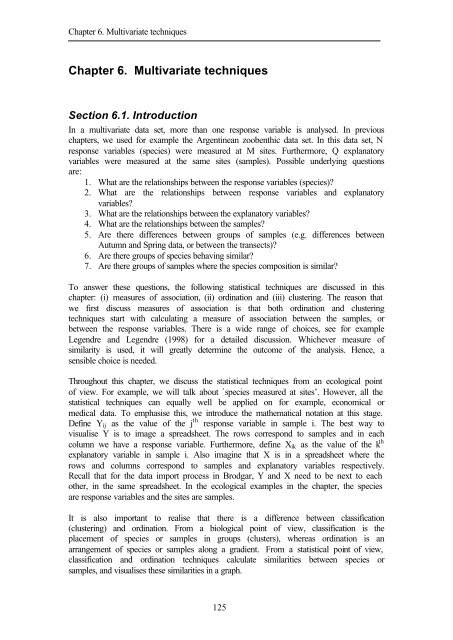
Chapter 6. Multivariate techniques

Chapter 6. Multivariate techniquesSection 6.2. Measures of association - CorrelationSuppose one has N observations on two variables Y and X, for example:• Number of a particular spider species (Y), and a habitat variable like moss cover(X) at N pitfall traps.• Abundance of a particular plant species (Y), and the value of Ph (X) in N soilsamples.• Total biomass of crabs (Y), and density of their burrows (X) at N forested sites.• Numbers of two zoobenthic species (Y and X) measured at 60 sites.The structure of the data is as follows:YXSample 1 Value ValueSample 2 Value Value… … …… … …Sample N Value ValueThe aim of correlation analysis is to find a linear relationship between Y and X; forexample:• Is there a linear relationship between the spider species and the habitat variable?• Is there a linear relationship between the plant species and the value of Ph?• Is there a linear relationship between crabs and burrow density?• Is there a relationship between the two zoobenthic species?Two tools to analyse these questions are the covariance and/or correlation function.Both determine how much the two variables covary (vary together):• If the first variable increases, does the second variable increase as well?• If the first variable increases, does the second variable decrease?• If the first variable decreases, does the second variable decrease as well?• If the first variable decreases, does the second variable increase?Mathematically, the covariance is defined as:N1Cov(Y,X) = ( Yi−Y)( Xi− X )N −1∑ j=1Where the bars above Y and X indicate mean values. As an example, we calculate thecovariance between the four zoobenthic species from the Argentine data. Thecovariances are given in Table 6.1. The diagonal elements in Table 6.1 are thevariances.126

Chapter 6. Multivariate techniquesstrength of the linear relationship between Y and X. To estimate it, observed data areused and therefore the estimator is called the sample correlation, or the Pearsonsample correlation function. It is a statistic and has a sample distribution. If one wouldrepeat the experiment n times, one would end up with n estimations of the correlationcoefficient. The most common used null hypothesis for the Pearson correlationfunction is:H 0 : Cor(Y,X) =0If H 0 is true, there is no linear relationship between Y and X. The correlation can beestimated from the data using equation (6.1), and a t-statistic or p-value can be used totest H 0 . The underlying assumption for this test is that Y and X are bivariate normallydistributed. This basically means that both Y and Xneed to be normally distributed. Ifeither Y or X is not normally distributed, the joint distribution is not normallydistributed neither. Graphical exploration tools can be used to investigate this. Thereare four options if non-normality is expected:1. Transform one or both variables.2. Use a different distribution.3. Use a more robust measure of correlation.4. Do not use a hypothesis test.Robust measures of correlation can be applied if the data are non-normal, nonbivariatenormal, standardisation does not help, or if there are non-linear relationships.One robust correlation function is the Pearson rank correlation. It is applied on ranktransformed data. The process is explained in Tables 6.3 and 6.4. The first table showsthe data of an artificial example. In the second table, each variable has been ranked.Originally the variable Y had the values 6 2 8 3 1. The first value, 6, is the fourthsmallest value. Hence, it rank value is 4. Ranking all values results in 4 2 5 3 1. Thesame process is applied on X. Spearman’s rank correlation is obtained by calculationthe Pearson correlation between the ranked values of Y and X.Table 6.3. Artificial data for Y and X.Y XSample 1 6 10Sample 2 2 7Sample 3 8 15Sample 4 3 3Sample 5 1 -5Table 6.4. Ranked artificial data for Y and X.Y * X *Sample * 1 4 4Sample * 2 2 3Sample * 3 5 5Sample * 4 3 5Sample * 5 1 1128

Chapter 6. Multivariate techniquesNote that the correlation techniques only detect monotonic relationships and not nonmonotonic,non-linear relationships. It is useful to inspect the correlation coefficientsbefore and after a data transformation. The Pearson correlation coefficient forms thebasis of multivariate techniques like principal component analysis and redundancyanalysis. The Spearman rank correlation is not yet available in Brodgar.Section 6.3. Measures of association – Chi-square distanceSuppose that an insect pollination study, the data in Table 6.5 were measured. Theunderlying questions in this study, is whether there is any association between thetype of insects and the colour of flowers. A Chi-square test is the most appropriate2test. The Χ statistic is calculated by: ∑− 2( O E)where O represents the observedEvalue and E the expected value. For the data in Table 6.5, the following steps arecarried out to calculate the Chi-square statistic. First the null hypothesis is formulated:H 0 : there is no association between the rows in Table 6.5.Formulated differently, insects are at random distributed over the flowers. If rows andcolumns are indeed independent (as suggested by the null hypothesis), the expectednumber of beetles in white flowers is 564 * (102/564) * (144/564), which is 26.04.Table 6.6 shows all the observed and expected values. The (O-E) 2 /E table is presentedin Table 6.7.The Chi-square statistic is equal to 115.03. The larger this value, the more unlikely isthe null hypothesis. The Chi-square statistic has (3-1)*(3-1)=2 degrees if freedom(df). The df are calculated using: (number of rows minus 1) times (number of columnsminus 1). Using a Chi-square table, the significance level for alpha=0.05 and 4 df is9.488. Hence, the null hypothesis is very unlikely. Based on the values in Table 6.7,the highest contribution to the Chi-square test was from beetles at white flowers,beetles at blue flowers and bees and wasps at blue flowers. The information in Table6.7 can be used to infer that beetles prefer white flowers but avoid blue flowers. Laterin this chapter, correspondence analysis is used to visualise this information.Table 6.5. Numbers of insects at flowers. Data from Ennos (2000). Statistical andData Handling Skills in Biology.Species White flower Yellow flower Blue flower TotalBeetles 56 34 12 102Flies 31 74 22 127Bees and wasps 57 103 175 335Total 144 211 209 564129

Chapter 6. Multivariate techniquesTable 6.6. Observed and expected values for the insects at flowers data. Values wereobtained using Excel.Species White flower Yellow flower Blue flower TotalBeetles 56 26.04 34 38.16 12 37.80 102Flies 31 32.43 74 103 22 47.06 127Bees and wasps 57 85.53 103 125.33 175 124.14 335Total 144 211 209 564Table 6.7. Contribution of individual cells to Chi-square statistic. Values wereobtained using Excel.Species White flower Yellow flower Blue flower TotalBeetles 34.46 0.45 17.61 52.52Flies 0.06 14.77 13.35 28.18Bees and wasps 9.52 3.98 20.84 34.33Total 44.04 19.20 51.79 115.03Chi-square distanceThe idea of the Chi-square statistic can be used to define similarity between species(response variables). The Chi-square distance between two species (responsevariables) is defined by:M 1 Z1jZ2 jD(Y,X)== Z+ + ∑ =( − )j 1Z+jZ1+Z2+The algorithm will create a matrix Z (of dimension 2xM) containing the data of thetwo species. Z 1j is the abundance of the first species at site j, and a `+’ refers to row orcolumn totals. The Chi-square metric is identical to the Chi-square distance, exceptfor the multiplication of the square root of Z ++ (total of Y and X). Table 6.8 shows theChi-square distances between the four zoobenthic species.2Table 6.8. Chi-square distances between the four zoobenthic species from theArgentine data. The abbreviations LA, HS, UU and NS refer to L. acuta, H. similes,U. uruguayensis and N. succinea. No transformation was applied. The values wereobtained from Brodgar and are dissimilarity coefficients; the smaller the value, themore similar.LA HS UU NSLA 0 1.6 2 3.7HS 1.6 0 2.4 3.4UU 2 2.4 0 4NS 3.7 3.4 4 0130

Chapter 6. Multivariate techniquesNote that U. uruguayensis and N. succinea have the highest Chi-square distances.Hence, these species behave the most similar, as judged by the Chi-square distancefunction. The disadvantage of the Chi-square distance function is that it is extremelysensitive to species that are highly abundant at only a few sites (abundant patchybehaviour). The underlying measure of association in correspondence analysis andcanonical correspondence analysis is the Chi-square distance function. Abundant andpatchy species will almost certainly dominate the first few axes of the ordinationdiagram.Section 6.4. Measures of association – Other functionsIn the previous sections, the covariance, correlation, Chi-square metric and Chisquaredistance functions were used to calculate associated between species orsamples. Traditionally, these functions are important for methods like linearregression, principal component analysis, correspondence analysis, redundancyanalysis and canonical correspondence analysis. However, the large number of zeroobservations (which is causing high correlations), non-linear relationships in ecologyand abundant patchy behaviour make these measures of association, and consequentlythe output of PCA, CA, RDA, and CCA, difficult to interpret.At this point, we should perhaps say a few words about the historical development ofordination techniques in ecology. In the mid 1950s, ordination techniques likeprincipal component analysis and Bray-Curtis ordination were used by ecologists(Goodall 1953; Bray and Curtis 1957). In the mid 1980s, correspondence analysis andcanonical correspondence analysis became popular in ecology, primarily because TerBraak (1985, 1986) gave it an ecological rationale (see Chapter 8), and provided easyto use software. Some scientists (and scientific journals) consider CA and CCA as“the” method to use. However, as mentioned earlier in this chapter, these methods arebased on the Chi-square distance function and this might not always be the bestoption. We also mentioned that PCA and redundancy analysis might not be the mostappropriate tools to analyse ecological data (double zeros, non-linearity). Another“school of scientist” has been working on non-metric multidimensional scaling(NMDS). The main advantage of NMDS is that a much wider range of measure ofassociation can be used. The disadvantage is that it is a so-called indirect gradientanalysis technique. CCA and RDA are direct gradient analysis techniques; responsevariables are directly linked to explanatory variables. Indirect gradient analysistechniques (PCA, CA, NMDS) only allow for the analysis of one data set (e.g.response variables), and linking the explanatory variables should be done afterwardsby using for example correlation techniques. However, Legendre and Gallagher(2001) showed that various other measures of association can be combined with PCA,CA, RDA and CCA. This combination leads to so-called distance based RDA (db-RDA transformations) and is discussed later in this chapter. Next, we discuss some ofthe measures of association that can be used in NMDS, and as db-RDAtransformations. For a detailed discussion, the reader is referred to Legendre andLegendre (1998) or Jongman et al. (1996).Besides the correlation and Chi-square distance functions, there are a large number ofother measures of association, for example the Similarity index of Jaccard (SJ),131

Chapter 6. Multivariate techniquesCoefficient of communication (CC), Similarity ratio (SR), Percentage similarity (PS),Euclidean distance (ED), squared Euclidean distance, Ochiai coefficient (OS), or theChord distance (CD). One of the confusing things with these measures of associationis that they appear (and re-appear) under different names. For example, the Ochiaicoefficient is also called the Cosine index, and another name for the Percentagesimilarity is the Sørenson index. Some of these are similarity coefficients, and othersare dissimilarity coefficients. A similarity coefficient means that 0 is not similar,whereas 1 is similar. Clustering methods typically work on measures of dissimilarityinstead of similarity. Possible transformations of a similarity matrix Z to adissimilarity matrix Z * are:1. Z * = max(Z) - Z2. Z * = |max(Z) – Z|3. Z * = sqrt( | max(Z) – Z | )Brodgar will automatically apply the most appropriate transformation, if one isrequired (e.g. for clustering). In most cases, this will be the first transformation.Jaccard indexTable 6.9 contains an artificial example of numbers (counts) of 5 species measured attwo sites. The Jaccard index considers the data as presence-absence, see Table 6.10.Using the data in Table 6.10, the algorithm for calculating the Jaccard index (JC)between sites 1 and 2 (which are now the two response variables), calculates thenumber of observations unique to site 1 (a), unique to site 2 (b), and the joint presencein sites 1 and 2 (c). The values for a, b and c are given in Table 6.11.Table 6.9. Artificial example of numbers (counts) of 5 species measured at two sites.Species Site 1 Site 2A 10 12B 7 0C 0 8D 0 8E 0 0Table 6.10. Transformation of data in Table 6.9 to presence (1) and absence (0).Species Site 1 Site 2A 1 1B 1 0C 0 1D 0 1E 0 0132

Chapter 6. Multivariate techniquesTable 6.11. Values unique to sites 1 and 2, and joint presence (1) and absence (0).Site 1Site 21 01 1 (=c) 1 (a)0 2 (=b) 1The Jaccard index (JC) between two variables is calculated as: JC = c / (a+b+c). Forthe data in Table 6.11 we have: JC= 1/(1+2+1)=0.25. Alternatively, the JC can becalculated by: JC = c / (A+B-c), where A is number of observations (in Table 6.10) insite 1 (=a+c=2), and B is the number of observations in site 2 (=b+c=3). Computersoftware (e.g. Brodgar) can be used to calculate the JC for every possiblecombination, and results can either be presented visually (e.g. using NMDS) or in atable. Table 6.12 shows the Jaccard index for the zoobenthic data. N. succinea and U.uruguayensis are very similar, as judged by the Jaccard index. Note that the jointpresence (component c) is important for this measure of association.Table 6.12. Jaccard index between the four zoobenthic species from the Argentinedata. The abbreviations LA, HS, UU and NS refer to L. acuta, H. similes, U.uruguayensis and N. succinea. No transformation was applied. The values wereobtained from Brodgar. The Jaccard values given by Brodgar (Multivariate-R Tools –Measures of association) are similarity coefficients; the larger the value, the moresimilar.LA HS UU NSLA 1 0.73 0.28 0.3HS 0.73 1 0.21 0.34UU 0.28 0.21 1 0.06NS 0.3 0.34 0.06 1Coefficients of community (CC)This coefficient is similar to the JC, except that it gives more weight to joint presence:CC = 2c / (A+B).Note that both the JC and CC treat the data as presence-absence data. Table 6.13 givesthe CC values for the zoobenthic species. There are minor differences compared to theJC.133

Chapter 6. Multivariate techniquesTable 6.13. Coefficients of community (CC) between the four zoobenthic speciesfrom the Argentine data. The abbreviations LA, HS, UU and NS refer to L. acuta, H.similes, U. uruguayensis and N. succinea. No transformation was applied. The CCvalues given by Brodgar are similarity coefficients; the larger the value, the moresimilar.LA HS UU NSLA 1 0.85 0.43 0.46HS 0.85 1 0.34 0.51UU 0.43 0.34 1 0.11NS 0.46 0.51 0.11 1Similarity ratio (SR)For presence-absence data, the Similarity ratio (SR) gives exactly the same results asthe JC. For other types of data, it takes into account the quantitative aspect of data aswell. Its mathematical formulation between two species Y and X is given by:SR(X,Y)=∑kY2k+∑∑kkYXkX2kk−∑kYkXkWhere the index k refers to samples. For presence-absence data, SR becomes theJaccard index. Table 6.14 shows the SR values for the Argentine data.Table 6.14. Similarity ratio between the four zoobenthic species from the Argentinedata. The abbreviations LA, HS, UU and NS refer to L. acuta, H. similes, U.uruguayensis and N. succinea. No transformation was applied. The SR values givenby Brodgar are similarity coefficients; the larger the value, the more similar.LA HS UU NSLA 1 0.34 0.18 0.04HS 0.34 1 0.09 0.16UU 0.18 0.09 1 0.06NS 0.04 0.16 0.06 1Percentage similarity (PS), alias Sørenson indexFor 0/1 data the percentage similarity (PS) is identical to CC. For other types of data,it takes into account the quantitative aspect of data as well. Its mathematicalformulation between two species Y and X is given by:134

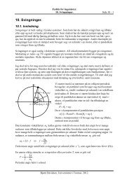
Chapter 6. Multivariate techniquesPS(X,Y)=200*Where the index k refers to samples.∑k∑kmin( Y , X )Yk+k∑kXkkEuclidean distanceSuppose we have numbers of 3 species (A, B and C) measured at 5 sites (1-5), seeTable 6.15. If we consider the species as axes, the 5 samples can be plotted in a 3-dimensional space, see Figure 6.4.1. The Euclidean distance between two sites i and jis calculated by:ED=3∑k = 1( Y−kiY kj2)Where Y ki is the abundance of species k at site i. It is easy to show that the Euclideandistance between sites 1 and 2 is the square root of 24, and between sites 3 and 4 it isthe square root of 14. Hence, the ED function indicates that sites 3 and 4 are moresimilar than sites 1 and 2, and this does make sense if you look at the threedimensionalgraph. However, sites 3 and 4 do not have any species in common,whereas sites 1 and 2 have at least one species in common, namely species A. Thisshows that for certain types of data, the Euclidean distance function is not the besttool to use, unless of course one wants to identify outliers. The Euclidean distancesbetween the four zoobenthic species are given in Table 6.16.Table 6.15. Artificial example of numbers of three species (A, B and C) measured at 5sites (1-5).1 2 3 4 5A 1 5 0 0 3B 0 2 3 0 2C 2 0 0 4 3135

Chapter 6. Multivariate techniquesC4153BA2Figure 6.4.1. Three-dimensional graph of abundance at 5 sites (response variables) of3 species.Table 6.16. Euclidean distances between the four zoobenthic species from theArgentine data. The abbreviations LA, HS, UU and NS refer to L. acuta, H. similes,U. uruguayensis and N. succinea. No transformation was applied. The Euclideandistance values given by Brodgar are dissimilarity coefficients; the smaller the value,the more similar.LA HS UU NSLA 0 456 439 465HS 456 0 282 275UU 439 282 0 59NS 465 275 59 0Orchiai coefficient and Chord distanceAs shown in the previous paragraph, absolute numbers influences the Euclideandistance function. To reduce this effect, the Orchiai coefficient (OS) or distance chord(CD) can be used. To obtain the Orchiai coefficient, imagine a line from the origin toeach site in Figure 6.4.1. The Orchiai coefficient between two sites (responsevariables) is then the angle between the lines of the corresponding sites. Simplegeometry is used to calculate it.136

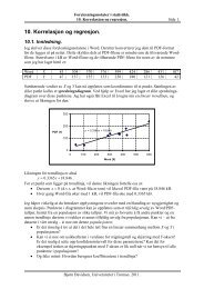
Chapter 6. Multivariate techniquesThe Chord distance between two sites (response variables) is obtained by drawing aunit circle around the origin in Figure 6.4.1, and calculating distances between theintersect points (these are the points were the circles and the lines intercept).Section 6.5. Measures of association – SummaryLegendre and Legendre (1998) give approximately 50 other measures of similarity,and this obviously raises the question when to use which measure of association. Theanswer to this question basically depends on (i) the underlying questions, (ii) the dataand (ii) characteristics of the association function. If you are interested in outliers, theEuclidean distance function is a good tool. But for ordination and clustering purposes,the Sørenson or Chord distance functions seem to perform well in practise, at leastbetter than the correlation and Chi-Square functions. Jongman et al. (1996) carried outa study in which various measures of association were applied to simulated ecologicaldata. Some of their results are reproduced in Table 6.17.Table 6.17. Characteristics of the (dis)similarity indices. Sensitivity for certainproperties of the data is indicated by:- non-sensitive; + sensitive; ++ and +++stronglysensitive. Results are from Jongman et al. (1996).AbbreviationQualitativeQuantitativeDissimilaritySimilaritySensitivity toSpeciesSensitivity toDominantSensitivity toSample TotalSimilarity Ratio SR * * * ++ ++ ++Percentage Similarity PS * * * ++ + +Cosine COS * * * + + -Jaccard index SJ * * ++ - -Coefficient of community CC * * + - -Cord distance CD * * * + + -Percentage Dissimilarity PD * * * ++ + +Euclidean distance ED * * * ++ ++ ++Squared Euclidean distance ED 2 * * * +++ +++ +++To show that is rather important to give some thoughts on the choice of measure ofassociation, we visualised all the distance matrices that were calculated for theArgentine zoobenthic data. Visualisation was done with NMDS, and results arepresented in Figure 6.5.1. Species close to each other represent species, which weresimilar, as judged by the measure of association. Note that the results indicate thatdepending on the measure of similarity, conclusions can fundamentally differ! Onlythe JC and CC give similar a outcome.137

Chapter 6. Multivariate techniquesCorrelationChi-square distanceAxis 2-0.5 0.0 0.5L.acutaU.uruguayensisH.similisN.succineaAxis 2-1 0 1 2 3L.acutaH.similisN.succineaU.uruguayensis-0.5 0.0 0.5Axis 1-1 0 1 2 3Axis 1Jaccard indexCommunity coefficientAxis 2-0.4 -0.2 0.0 0.2 0.4 0.6N.succineaH.similisL.acutaU.uruguayensisAxis 2-0.6 -0.4 -0.2 0.0 0.2 0.4U.uruguayensisL.acuta H.similisN.succinea-0.4 -0.2 0.0 0.2 0.4 0.6Axis 1-0.6 -0.4 -0.2 0.0 0.2 0.4Axis 1Similarity RatioEuclidean distanceAxis 2-0.4 -0.2 0.0 0.2 0.4 0.6N.succineaH.similisL.acutaU.uruguayensisAxis 2-100 0 100 200 300 400H.similisN.succineaU.uruguayensisL.acuta-0.4 -0.2 0.0 0.2 0.4 0.6-100 0 100 200 300 400Axis 1Figure 6.5.1. NMDS graphs for various measures of association between the zoobenthicspecies.Axis 1138

Chapter 6. Multivariate techniquesSection 6.6. Measures of association – BrodgarWe now explain how to get the measures of association, and the NMDS graphs inBrodgar. To calculate measures of association, or indeed apply ordination orclustering, click on the main menu button “Multivariate”. It will show the upper leftpanel in Figure 6.6.1.Figure 6.6.1. Multivariate techniques available in Brodgar.For the moment, we are only interested in the “Measures of association” option (under‘R tools’) in the lower left panel in Figure 6.6.1. If you select it and click on “Go”, thewindow in Figure 6.6.2 appears. You have the following options:Association between samples or variables. Apply the measure of association on thevariables or samples.Measures of similarity. Make sure that your selection is valid for the data. Forexample, Brodgar will give an error message if you apply the Chi-square distance139

Chapter 6. Multivariate techniquesfunction on samples with a total of 0. Also consider the transformation andstandardisation, which you might have selected during the data import process. Forexample, a log transformation might result in negative numbers, in which case it doesnot make sense to select the Jaccard index function. There are only a few measures ofassociation that can cope with normalised data (e.g. the correlation matrix).Summarising, if you get an error message, please check whether the selected measureof association is valid.Select variables and samples. Click on “Select all variables” and “Select all samples”to use all the data. The “Store” and “Retrieve” functions are handy as well.Under settings, items like the title and graph name can be specified.Once, the appropriate selections have been made, click on the “Go” button in Figure6.6.2. This results in Figure 6.6.3. It shows the NMDS ordination graph, which wasobtained by applying the R function cmdscale to the selected dissimilarity matrix. Theactual values of the measure of association can be obtained from the menu in Figure6.6.4; click on “Numerical output”. The measures of association can either be openedin a text file, or copied to the clipboard as tab separated data, and from there it can bepasted into Excel. You can also access these values in your project directory. Look forthe file \YourProjectName\meassimout.txt. You can even open the file similarity.R(which is in the Brodgar installation directory) and source all the code directly in R.Figure 6.6.3. Selection of variables and settings for measures of association.140

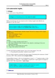
Chapter 6. Multivariate techniquesFigure 6.6.4. Selection of variables and settings for measures of association.Section 6.7. Ordination - IntroductionThe aim of dimension reduction methods is twofold. First of all, these techniques tryto reduce the large number of variables into a few new, easy to interpret, variables. Itis hoped that these new variables summarise the main features of the originalvariables. Secondly, dimension reduction techniques can be used to reveal patterns inmultivariate data, which are not picked up in univariate analyses. These methodsresult in easy to read pictures, which partly explain their popularity. Another reason isthe availability of easy-to-use software. Dimension reduction techniques are alsoreferred to as ordination methods, gradient analysis, latent class models, amongothers. We start by explaining the basic underlying idea of dimension reduction.Probably, the best way to do this is to use one of the oldest techniques available,namely Bray-Curtis ordination. The mathematical calculations required for thismethod are so simple that a pen and paper can do the job.Bray-Curtis ordinationTable 6.18 shows the Sørenson distances between the four zoobenthic species. Thehigher the value, the more similar are the corresponding species. Our goal is tovisualise these distances along a line. The way Bray-Curtis ordination (or: Polarordination) does this, is as follows. First, it is searching for the highest value, which is96. This is between L. acuta and N. succinea. It will then place these two species atthe ends of a line (Figure 6.7.1). The length of this line is 1 unit. To determine theposition of a third species, say U. uruguayensis, two circles are drawn. The first circlehas as center the left endpoint, and the second circle has the right endpoint as center.The radius of the first circle is given by the Sørenson distance between L. acuta andU. uruguayensis, which is 88. The radius of the second circle is determined by theSørenson distance between N. succinea and U. uruguayensis, which is 93 (Figure6.7.1). The position of U. uruguayensis on the line is determined by verticalprojection the interception of the two circles on the line (Figure 6.7.1). The same141

Chapter 6. Multivariate techniquesprocess is repeated for the other species. Further axes can be calculated, see McCuneand Grace (2002), and Beals (1984) for details.Table 6.18. Sørenson distances between the four zoobenthic species from theArgentine data. The abbreviations LA, HS, UU and NS refer to L. acuta, H. similes,U. uruguayensis and N. succinea. No transformation was applied. The values wereobtained from Brodgar.LA HS UU NSLA 0 71 88 96HS 71 0 89 88UU 88 89 0 93NS 96 88 93 0L. acutaN. succineaCircle withradius 88Position U.uruguayensisCircle withradius 93Figure 6.7.1. Underlying principle of Bray-Curtis ordination.Instead of the Sørenson distances, various other measures of similarity can be used inpackages like Brodgar and PC-Ord. General options are the Sørenson, RelativeSørenson, Euclidean and relative Euclidean distances. Relative means that sampletotals are standardized to one. For example, if Bray-Curtis is applied to variables, theneach row (sample) is divided by the row sum, prior to the analysis. This reduces theeffect of abundant sites. If the relative Sørenson index is applied, make sure that youare not dividing by zero.142

Chapter 6. Multivariate techniquesThere are different ways to select the endpoint of the line (or: axis). The originalmethod (which is also the default) was sketched in Figure 6.7.1, namely by selectingthe pair of variables that had the highest measure of association. However, thisapproach tends to result in an axis that has one or two species on one side, and all theother species on the other side of the axis. The isolated species are likely to beoutliers. Indeed, Bray-Curtis ordination with the original method to select endpoints isa useful tool to identify outliers (provided these outliers have a low similarity with theother variables). An alternative is to select your own endpoints. This is called“subjective”. It allows you to test whether certain variables are outliers. The thirdoption was developed by Beals (1984) and is called “variance-regression”. The firstendpoint calculated by this method, is the point that has the highest variance ofdistances to all other points. An outlier will have large distances to most other points,and therefore the variation in these distances is small. McCrune and Grace (2002) saidthe following about the first endpoint as “…it is at the long end of the main cluster inspecies space.”. Getting the second endpoint is slightly more complicated. Supposethat species 1 is the first endpoint. The algorithm will in turn, consider each of theother species as an endpoint. In the first step, it will take species 2 as the secondendpoint. Let D 1i be the distance of species 1 to all other species (except for species 1and 2). Furthermore, let D 2i be the distance of species 2 to all other species. Thenregress D 1i on D 2i and store the slope. Repeat this process for all other trial endpoints.The second endpoint will be the species that has the most negative slope. McCune andGrace (2002) justify this approach by saying that the second endpoint is at the edge ofthe main cloud of species, opposite to endpoint 1.The Bray-Curtis ordination using thezoobenthic data and the Sørenson distances in Table 6.18 is presented in Figure 6.7.2.The positions of the species along the axis are represented by dots. The species namesare plotted with an angle of 45 degrees above and below the points. Results indicatethat H. similes, and U. uruguayensis are similar (appear at the same sites). Thevariance explained by the axis is 41%.Bray-Curtis ordinationN.succineaH.similisU.uruguayensisL.acuta0 20 40 60 80 100Axis 1Figure 6.7.2. Bray Curtis ordination using the Sørenson index, applied to thezoobenthic data from Argentina. The original method to select endpoint was used,and 1 axis was calculated.143

Chapter 6. Multivariate techniquesBray-Curtis ordination is one of the oldest ordination methods in ecology. Despitevarious critical reviews, it is still used by scientists. Nowadays, it might be difficult toget a paper published in a scientific journal, that solely uses Bray-Curtis ordination,but we do think that it is a useful multivariate data analysis tool. Furthermore, it is“the perfect example” to explain the underlying principle of dimension reductiontechniques to students.Obviously, more complicated multivariate techniques have been developed andapplied in ecology since the mid 1950s, e.g. principal component analysis (PCA),correspondence analysis (CA), redundancy analysis (RDA), canonical correspondenceanalysis (CCA), canonical correlation analysis (CCOR), partial RDA, partial CCA,variance partitioning or discriminant analysis (DA). Some of these techniques arediscussed later in this chapter.Bray-Curtis ordination in BrodgarTo carry out Bray-Curtis ordination in Brodgar, select it in the window in Figure 6.6.1(Multivariate – R Tools – Bray Curtis ordination) and click on the “Go” button. Theoptions for Bray-Curtis ordination are given in the two panels in Figure 6.7.3. Theuser can make the following selections under the “Variables” panel.Visualise association between samples or variables. Apply Bray-Curtis ordination onthe variables or samples. We selected variables.Measure of similarity. These were discussed in Section 6.7. Make sure that yourselection is valid for the data. For example, Brodgar will give an error message ifthere are sites with no species at all, and you select the relative Sørenson index.Select variables and samples. Just click on “Select all variables” and “Select allsamples” if you want to use all the data. The “Store” and “Retrieve” functions arehandy as well.Methods to select endpoints. These were discussed in the previous section.Setting axes limits. Brodgar will automatically scale the axes. If you use long speciesnames, part of the name might fall outside the graph. In this case, you might want tochance the minimum and maximum values of the axes. The input needs to be of theform: 0,100,0,100 for two axes, and 0,100 for 1 axis. Note the comma separation!Number of axes. Either 2 axes (default) or 1 axis is calculated. The algorithm inBrodgar is described in McCrune and Grace (2002). To obtain a second axis, residualsdistances are obtained before calculation on the second axis starts. The size of thegraph labels and angle of the labels (for 1 axis only) can be changed. Other optionsinclude the title, labels and graph name.Numerical output is available from the menu in the Bray-Curtis window (not shownhere). Other information available is the distance matrix and the scores. If 2 axes arecalculated, Brodgar will also present the correlations between the original variablesand the axes in a biplot.144

Chapter 6. Multivariate techniquesFigure 6.7.3. Bray Curtis options in Brodgar.Section 6.8. OrdinationIn the previous section, Bray Curtis ordination was explained, and we mentioned a listof more recently developed, popular and sophisticated multivariate techniques. Someof these techniques (e.g. canonical correspondence analysis) are extremely popular inecology, although an economist might never have encountered them before. Thenames themselves also depend on the field of application; an ecologist will talk aboutPCA but in climatology this is called empirical orthogonal functions (EOF) analysis.PCA, CA, DA and MDS can be used to analyse data without explanatory variables,whereas CCA and RDA require a division of the variables in response andexplanatory variables. In CCOR the variables are also divided in two sets, but notnecessarily in response and explanatory variables.The underlying principleNearly all dimension reduction techniques create linear combinations of the data:Z i1 = c 11 Y i1 + c 12 Y i2 + … + c 1N Y iN145

Chapter 6. Multivariate techniquesThis can be imagined as multiplying each column (variable) in the spreadsheet with aparticular value, followed by a summation over the columns. The linear combination,Z 1 , is a vector of length M (number of samples), and is called a principal component,gradient or axis. The underlying idea is that the most important features in the Nresponse variables are caught by the new variable Z. Obviously, one componentcannot represent all features of N response variables, and further components can beextracted. This means that a second component is calculated:Z i2 = c 21 Y i1 + c 22 Y i2 + … + c 2N Y iNMost dimension reductions techniques are designed in such a way that the informationin Z 2 is independent of Z 1 , and that Z 1 is more important. Nearly all dimensionreduction techniques use the phrase “eigenvalues”. This is a measure of how muchinformation each component contains in terms of the total variation in the data. Themultiplication factors c ij are called loadings. The difference between PCA, DA andCA, is the way these loadings are calculated. In RDA, CCA and CCOR, a second setof variables is taken into account in calculating the loadings.PCAPCA is one of the oldest and most common used ordination methods. The reason forits popularity is perhaps its simplicity. Before introducing PCA, we clear up a fewmisconceptions. PCA cannot cope with missing values, it does not require normality,it is not a hypothesis test, and there is no clear distinction between response variablesand explanatory variables.There are various ways to introduce PCA. Our first approach is based on Shaw(2003), who used the analogy with shadows to explain PCA. Imagine giving apresentation. If you put your hand in front of the overhead projector, your 3-dimensional hand will be projected on a 2-dimensional wall or screen. The challengeis to rotate your hand such that the projection on the screen resembles the originalhand as good as possible. This idea of projection and rotation brings us to a morestatistical approach of introducing PCA. The upper left panel in Figure 6.8.1 shows ascatterplot of the species richness and NAP variables of the RIKZ data. There is aclear negative correlation between these two variables. The upper right panel showsthe same scatterplot except that both variables are now mean deleted. To furtherreduce the effect of different scales, units and spread in the two variables, a scatterplotof normalised data is presented in the middle left panel in Figure 6.8.1. In the middleright panel, the same scatterplot is presented except that numbers are used instead ofpoints. We also used axes with the same range (from –3.5 to 3.5). Suppose that wewant to have two new axes such that the first axis represents most information, andthe second axis the second most information. In PCA, ‘most information’ is definedas the largest variance. The diagonal line from the upper left to the lower right in theright-middle panel in Figure 6.8.1 is this first new axis. Projecting the points on thisnew axis results in the axis with the largest variance; any line with another angle withthe x-axis will have a smaller variance. The additional restriction we put on the newaxes is that the axes should be perpendicular to each other. Hence, the dotted line inthe same panel is the second axis. The lower left graph shows the same graph as themid-right panel; except that the new axes are presented in a more natural direction.This graph is called a PCA ordination plot. The axes in PCA are sign independent146

Chapter 6. Multivariate techniques(they can be mirrored in each axis), and therefore the PCA ordination plot is mirrored(and rotated) in the axes compared to the original data.In the same way as the 3-dimensional hand was projected on a 2-dimensional screen,we can project all the observations onto the first PCA axis, and omit the second axis.This is done in the lower right panel in Figure 6.8.1. To avoid cluttered text, a certainamount of vertical jittering was applied. PCA output (which is discussed later) showsthat the first new axis represents 76% of the information in the original scatterplot.To go from the upper left to the lower left graph in Figure 6.8.1, we normalised androtated the data. The two new axes are given by:Z i1 = c 11 R i + c 12 NAP i and Z i2 = c 21 R i + c 22 NAP iOr in matrix notation: Z = XC, where C contains the rotation factors, X the originalvariables and Z the principal components. The general formulation of PCA is asfollows. Suppose we have N variables, where we make no distinction betweenresponse and explanatory variables. PCA calculates a linear combination of the Nvariables:Z i1 = c 11 Y i1 + c 12 Y i2 + … + c 1N Y iNThe algorithm of PCA estimates the coefficients c 11 ,..,c 1N such that the vector Z 1 hasmaximum variance. The coefficients c ij are called factor loadings. The idea ofcalculating a linear combination of variables is perhaps difficult to grasp at first.However, we have seen this before. Remember the richness index function, or totalabundance index function (Chapter 5). These are all linear combinations of theoriginal variables, and summarise a large number of variables with one indexfunction. The algorithm also estimated a second axis:Z i2 = c 21 Y i1 + c 22 Y i2 + … + c 2N Y iNThe variance in Z 2 is smaller. In applying PCA, one hopes that the variance of mostcomponents is negligible, and that the variation in the data can be described by a few(independent) principal components. Hence, instead of N original response variables,we end up with 2 or 3 principal components, which hopefully represent 70%-80% ofthe information in the data.Prior to the analysis, the PCA algorithm either mean deletes or normalises eachvariable. Hence, the Y values in the above formula are not the original variables, butare standardised. Later in this section, we show that a PCA applied to mean deleteddata visualises covariances between variables, whereas if normalised variables areused, the results show the correlations between variables. If the variables aremeasured in different units, or have a wide range in variation, it is better to base thePCA on the correlation matrix. Most software packages use the correlation matrix bydefault. We advise to use the correlation matrix, unless one has a good reason not todo so.147

Chapter 6. Multivariate techniquesR0 5 10 15 20R-5 0 5 10 15-1.0 -0.5 0.0 0.5 1.0 1.5 2.0NAP-1.5 -1.0 -0.5 0.0 0.5 1.0 1.5 2.0NAP22R-1 0 1 2 3R-3 -2 -1 0 1 2 3954126 117 317842 36 34 19 2538 404544 1031 16301526 1832 433537 41 2913 2 14 27 242823 20 21 39331-1 0 1 2NAP-3 -2 -1 0 1 2 3NAPaxis 210-1314238 323640 134516 30433415356 37 237 2419442641171014 2718 24202558 2928213312111393922-1 0 1axis 1R-0.2 -0.1 0.0 0.1 0.22211 315 9 6 71216 15 1017 18 23 24 2834 30 4336252113 27 20431 32 35 374238 4045 4419 82641 2 14 29 39 33-0.4 -0.3 -0.2 -0.1 0.0 0.1 0.2 0.3Figure 6.8.1. The underlying principle of PCA using the RIKZ data. The upper leftgraph shows a scatterplot of richness and NAP, the upper right is a scatterplot of thesame variables but now mean deleted. The middle left graph is a scatterplot ofnormalised richness and NAP. The middle right graph shows two new axes. The lowerleft graph contains the two PCA axes. The lower right is the projection of the points onthe first axis. A certain degree of jittering was applied.Axis 1148

Chapter 6. Multivariate techniquesMathematical background of PCAHaving presented two relatively easy introductions to PCA, we do feel it is necessaryto present PCA in a mathematical context as well. Readers not familiar with matrixalgebra might skip the next few paragraphs and continue with the illustration of PCA.We discuss two mathematical derivations of PCA.PCA as an eigenvalue decompositionThe aim of PCA is to calculate an axis Z 1 = Yc 1 that has maximum variance. Becausethe mean of the Y’s is zero, the variance of Z 1 is given by Z 1 ’Z 1 = c 1 ’Y’Yc 1 . Anaspect we have not mentioned so far is that the factor loadings are not unique. If asecond axis Z 2 = Yc 2 is calculated, then both c 1 and c 2 can be multiplied with 10,resulting in axes which are independent as well. Therefore, a restriction on the factorloadings is applied: c i ’c i = 1 for all i. This leads to the following optimisation problemfopr the first axis:Maximise var(Z 1 ) = Z 1 ’Z 1 = c 1 ’Y’Yc 1 , subject to c i ’c i = 1.This restricted maximisation can be solved with the Lagrange multiplier method:L = c 1 ’Y’Yc 1 – ? (1 – c 1 ’c 1 )The maximisation is with respect to the unknown parameters c 1 and ?. Taking thederivative of L with respect to ? and setting it to zero ensures that the restriction c i ’c i= 1 is met. The derivative of L with respect to c 1 is given by: 2Y’Yc 1 -2?c 1 . Setting itto zero results in:2Y’Yc 1 = 2?c 1 => (Y’Y – I?) c 1 = 0 => (S- I? * ) c 1 = 0where ? * = ?/(M-1), M the number of samples, S is the correlation matrix if Y isnormalised, and the covariance matrix if Y is centred. The expression (S- I? * ) c 1 = 0 isthe eigenvalue decomposition of S, ? * is the first eigenvalue and c 1 is the eigenvector.The eigenvalue decomposition for all axes is given by: (S- I? * ) C = 0. Hence, thefactor loadings are obtained by an eigenvalue decomposition of the correlation (or:covariance) matrix. Once factor loadings are estimated, the principal components areobtained from Z i = Yc i for all i. The eigenvalue decomposition allows for differentoptions to rescale loadings and scores, but the reader is referred to Jongman et al.(1996) or Legendre and Legendre (1998) for details. The motivation to present theeigenvalue decomposition here is that it justifies the iterative algorithm presented inthe next paragraph, and this algorithm is used to explain RDA in the next section.PCA as an iterative algorithmThe last approach to explain PCA is by using an iterative algorithm, which waspresented in Jongman et al. (1996) and Legendre and Legendre (1998), and referencesin there. The algorithm has the following steps.1. Normalise (or centre) the variables in Y (variables are in the columns).2. Obtain initial scores z (e.g. by a random number generator).3. Calculate new loadings: c = Y’z’.4. Calculate new scores: z = Yc.149

Chapter 6. Multivariate techniques5. For second and higher axes: make z uncorrelated with previous axes using aregression analysis.6. Scale z to unit variance: z* = z/? where ? is the standard deviation of thescores. Set z equal to z*.7. Repeat steps 2 to 6 until convergence.8. After convergence, divide ? by M-1.Once the algorithm is finished, the factor loadings c and principal components z(scores) are identical to those obtained from the eigenvalue decomposition. To derivethis relationship, substitute the expression in step 4 into 6, and then use 3. Theresulting expression is of the same structure as the eigenvalue decomposition.Illustration of PCATo illustrate PCA, we use the famous Bumpus sparrow data. This data set consists of5 morphological variables taken from approximately 50 sparrows that were caught inJapan after a major storm. Half of the birds survived, and the question is whetherbeing a big bird increases survival chances. The morphological variables were totallength, alar length, length of beak and head, length of humerus and length of keel ofsternum. As a general rule of thumb, PCA tends to produce good results if the originalvariables are highly (>0.5) correlated, where ‘good’ means that only a few axesrepresent most of the information. Hence, before applying PCA, the correlation matrixshould always be inspected. For the Bumpus data, the correlations are relatively high(Table 6.19), and therefore we expect to find a PCA in which the first two axesexplain a reasonable amount of information.Table 6.19. Correlations between the variables in the Bumpus data. The notation total,alar, beak/head, humerus and sternum refer to the morphological variables totallength, alar length, length of beak and head, length of humerus and length of keel ofsternum.Total Alar Beak/Head Humerus SternumTotal 1Alar 0.73 1Beak/Head 0.66 0.67 1Humerus 0.65 0.77 0.76 1Sternum 0.61 0.53 0.53 0.61 1The outcome of the PCA algorithm is as follows:Z 1 = 0.45 Total + 0.46 Alar + 0.45 Beak/Head + 0.47 Humerus + 0.40 SternumZ 2 = -0.01 Total + 0.30 Alar + 0.33 Beak/Head + 0.19 Humerus - 0.88 SternumThe traditional way of presenting results of PCA is to plot Z 1 versus Z 2 , see Figure6.8.2.150

Chapter 6. Multivariate techniquesaxis 2-1 0 1 2 337302521311011261835 17334411632 2019 2224 36473 38137 2345842 4327 12 482 15285 1 44 649 9394629403414-4 -2 0 2 4Figure 6.8.2. First two axes obtained by PCA for Bumpus data. Numbers refer to thesamples.axis 1One of the problems with PCA is to decide how many components to present, andthere are various rules of thumb. The first rule is the “80% rule”; present the first kaxes that explain 80% (cumulative) of the total variation. Another option is a screeplot of the eigenvalues (Figure 6.8.3). In such a graph, all the eigenvalues are plottedas bars or vertical lines, and hopefully there is an “elbow” effect. The justification isthat the first k axes explain most information, whereas axes k+1 and higher onlyrepresent a small amount of variation. A scree plot of the eigenvalues would thenshow a change at the k th eigenvalue, also called an elbow effect. This would justifyplotting only the first k axes. However, in most scientific publications one onlypresents the first two axes, and occasionally the first four axes. If the first few axesexplain a low percentage, then it might be worthwhile to investigate whether there areoutliers, the relationships between variables are linear, consider a transformation oraccept the fact that ecological data are noisy.0.723xVariances0 1 2 30.8290.9070.9671Comp. 1 Comp. 2 Comp. 3 Comp. 4 Comp. 5Figure 6.8.3. Eigenvalues for the Bumpus data obtained by PCA. The elbow rulesuggests presenting only the first axis. The graph was made in R.151

Chapter 6. Multivariate techniquesBiplotFigure 6.8.2 showed the general presentation of PCA as a plot of Z 1 against Z 2 .Interpretation of the plot is difficult, and the biplot was developed to simplify this. Wedo not present the mathematics behind the biplot, and the interested reader is referredto Jongman et al. (1996) or Legendre and Legendre (1998). Instead, we discuss howto interpret a biplot.A biplot is a visualisation tool to present results of PCA. There are various options forthe PCA biplot and this is called the scaling process. Depending on which aspect ofthe data one is interested, loadings and scores can be slightly modified. We suggeststicking to the default settings of packages like Brodgar and CANOCO. In the defaultscaling and interpretation, we have arrows (or lines) for variables (species) and pointsfor samples. Long lines indicate important variables. Lines pointing in the samedirection indicate that the corresponding variables are highly correlated with eachother. Lines pointing in opposite direction refer to variables, which are negativelycorrelated. Lines that have an angle of 90 degrees mean that the variables areuncorrelated. Points can be projected perpendicular on the lines, and indicate whetherthe sample has a high or low value for the variable. The basic points to do are (i)compare the directions of the lines, (ii) focus on the longer lines, (iii) compare linesand points, and (iv) compare the points with each other. If an alternative scaling isused, the interpretation is different (Legendre and Legendre 1998). Figure 6.8.4 showsthe PCA biplot for the Bumpus data. The results suggest that length of keel of sternumhas the `lowest’ correlation with the other variables, which are all highly correlatedwith each other. One can identify which samples had high values and which sampleshad low values.So far, PCA has ignored the extra information, which birds survived and which not.One way to use this information is by labelling the samples in the biplot by 1(survived) and 0 (did not survive). This is a rather cumbersome way, and techniqueslike discriminant analysis and redundancy analysis are considerably better tools totake such information into account.1axis 201110110001 00101 0011110011 1 01 110 11 010 100 01BeakHead AlarHumerusTotalKeelSternum-11-1 0 1axis 1Figure 6.8.4. PCA biplot for Bumpus data, obtained by Brodgar.152

Chapter 6. Multivariate techniquesNumerical output in PCAFinally, we discuss the numerical output of PCA (Table 6.20). The first axis explains72.3% of the variation in the data, and the second axis 10.63%. Together, the first twoaxes explain 83% of the variation in the data. Brodgar scales the eigenvalues such thatthe total sum is equal to 1. Other packages might do the same (CANOCO), or not (S-PLUS, R).Table 6.20. Numerical output of PCA applied to the Bumpus data. The eigenvaluesare scaled such that the sum of all eigenvalues is 1.Axis Eigenvalue Eigenvalue as % Eigenvalue as cumulative %1 0.723 72.32 72.322 0.106 10.63 82.953 0.077 7.73 90.674 0.060 6.03 96.715 0.033 3.29 100.00Missing valuesPCA and most other multivariate methods discussed in this chapter cannot cope withmissing values. Missing values must be replaced by a sensible estimate (e.g. meanvalue of the response variable).Explanatory variablesIn this paragraph, we set the tune for redundancy analysis. The left panel in Figure6.8.5 shows the biplot for the Argentine zoobenthic data. We applied a square roottransformation prior to the analysis. Results indicate that L. acuta and U.uruguayensis are correlated with each other, and that these two species were mainlyabundant at the transect B sites. Furthermore, N. succinea was mainly measured attransect C sites. The first two axes explain 68% of the variation in the data. In theright panel in Figure 6.8.5, we zoomed in, and superimposed the explanatory variables(mud content, medium sand, etc.). The line for an explanatory variables was obtainedby drawing a line from the origin to a point (c 1 ,c 2 ), where c 1 is the correlation betweenthe first axis and the explanatory variable, and c 2 with the second axes. A long lineindicates that the explanatory variable is highly correlated with at least one of theaxes. In this case, only medium sand has a reasonable long line; its correlation withthe first axis is approximately –0.5. However, suppose that the major gradients in thespecies data are not related to the environmental variables, and that the third andfourth PCA axes are related to the environmental variables. In such cases we wouldnot detect it in Figure 6.8.5. Redundancy analysis is a much better way to incorporateinformation on explanatory variables.An interesting extension of PCA is PCA-regression. In this method, the first few (say4) components are extracted and used as explanatory variables in a multiple linear153

Chapter 6. Multivariate techniquesregression. Using estimated regression parameters and loadings, it can be inferredwhich of the original variables are important.10.5axis 20C7C1A7B10 A3C6 C8B3 B4 B5 B2 B3 A1 A6C5 N.succineaB1 A5A8U.uruguayensis B7A4 A5 B6A9A2A1A6C9B4 A8 A2C9B6 A7 B8 B5B7C10B9C3 C10A4 A3A9A10 C2C5 C4C7C3 C6B1B8C2C1L.acutaB9 C8B2axis 20-0.5U.uruguayensisMedSandL.acutaFineSand TimeOrganMatMud-1B10A10C4H.similis-1 0 1axis 1-1 -0.5 0 0.5Figure 6.8.5. Left panel: PCA biplots for Argentine zoobenthic data. Right panel:Zoomed in biplots with superimposed explanatory variables.axis 1H.similisShortcomings and db-RDA transformationsThe two major problems with PCA are (i) that it measures linear relationships becauseit is based on the correlation or covariance coefficient, and (ii) double zeros. The lastphrase refers to species being absent at most sites and as a result have a highcorrelation.Legendre and Gallagher (2001) showed that various other measures of association canbe combined with PCA, namely the Chord distance, Hellinger distance, and two Chisquarerelated transformations. By using for example the Chord distance, the resultingbiplot presents a 2-dimensional representation of the Chord distance matrix.Section 6.9. Redundancy analysisIn the previous section, it was shown that PCA is useful tool to visualise correlationsbetween variables, but the explanation of the results in terms of explanatory variablesis cumbersome. Redundancy analysis (RDA) is an interesting extension of PCA thatexplicitly takes account of explanatory variables.A first approach to explain RDA is to ignore all the formulae and discuss how tointerpret the graphical and numerical output. The graphical output consists of twobiplots on top of each other, and is called a triplot. Explanatory variables arerepresented by lines or arrows, species (response variables) by lines or labels, andsamples by points or labels. The interpretation is identical to the PCA biplot, and anexample is presented later in this section.154

Chapter 6. Multivariate techniquesA second approach to explain RDA is as follows. PCA calculates the first principalcomponents as:Z i1 = c 11 Y i1 + c 12 Y i2 + … + c 1N Y iNRedundancy analysis is some sort of PCA in which one requires that the componentsare also linear functions of explanatory variables:Z i1 = a 11 X i1 + a 12 X i2 …… + a 1q X iQHence, the axes in RDA are not only a linear combination of the response (!)variables, but also of the explanatory variables. It is as if you would tell the computerto apply a PCA, but only show that information in the biplots, which can be (linearly)related to the explanatory variables. Further axes are obtained in the same way. RDAcan be applied if there are N response variables measured at M sites and Qexplanatory variables measured at the same sites. Note that this technique requires anexplicit division of the variables into response and explanatory variables.A more mathematical explanation of RDA requires the iterative algorithm for PCA,which was presented in the previous section. The algorithm has the following steps:1. Normalise (or centre) the variables Y (variables are in columns), andnormalise the explanatory variables X (variables are in columns).2. Obtain initial scores z (e.g. by a random number generator).3. Calculate new loadings: c = Y’z’.4. Calculate new scores: z = Yc.5. For second and higher axes: make z uncorrelated with previous axes using aregression analysis.6. Apply a linear regression of z on X and set z equal to the fitted values.7. Scale z to unit variance: z* = z/? where ? is the standard deviation of thescores. Set z equal to z*.8. Repeat steps 2 to 7 until convergence.9. After convergence, divide ? by M-1.The only extra steps are normalisation of X and the regression step in 6. The effect ofthis regression step is that only the information in z that is related to X is pertained. Itensures that the scores z are indeed a linear combination of the explanatory variables.Illustration of RDAAn example for the Argentine zoobenthic data is given in Figure 6.9.1. We only usedthe explanatory variables mud, medium sand and time. Results indicate that U.uruguayensis is highly correlated with medium sand, and the sites in transect A aremuddy. Time does not have an important role.155

Chapter 6. Multivariate techniques1axis 20-1B7A3 A10 MudB9 A2 C3 C10 A8B6 C9C4A4A1 A9B4B10A7 B5C8C2B8 A5A6 C7B3 L.acuta B7 H.similisC5 A3 C6A10B2 B9 A2 C3 C10 A8C1B1A4A1 A9B6 C9MedSand Time C4U.uruguayensis B4B10A7 B5C8C2B8 A5A6 C7B3N.succineaC5 C6B2C1B1-1 0 1Figure 6.9.1. RDA triplot for Argentine zoobenthic data. Square root transformedspecies data were used.axis 1The numerical output of RDA for the Argentine data (Table 6.21) shows that the firsttwo axes explain 98.98% of the variation in the data that can be explained with all theexplanatory variables. This is the row labelled ‘eigenvalue as cumulative percentageof the sum of all eigenvalues’. Hence, the first two axes are a good representation ofwhat can be explained with all the explanatory variables. Since we only used 3variables, this is nothing special. The third row is more interesting. It shows that thefirst two axes explain 18.5% of the variation in the species data that can be explainedwith the two axes. The sum of all canonical eigenvalues indicate that all explanatoryvariables used in the analysis explain 19% of the variation in the species data. Hence,we clearly missed a few important explanatory variables in this analysis.Table 6.21. Numerical output of PCA applied to the Argentine data. The sum of allcanonical eigenvalues is 0.19 and the total inertia is 1.Axis 1 Axis 2Eigenvalue 0.156 0.028Eigenvalue as % inertia 15.604 2.849Eigenvalue as % inertia, cumulative 15.604 18.453Eigenvalue as percentage of sum of all canonical 83.698 15.280eigenvaluesEigenvalue as cumulative percentage of sum of allcanonical eigenvalues83.698 98.978Nominal variables, forward selection and Monte-Carlo significance testsSoftware packages like Brodgar and CANOCO deal slightly different with nominalvariables, and this is discussed next using an artificial example. Suppose that156

Chapter 6. Multivariate techniquesabundances of two species were measured at 5 sites and that sampling took place overa period of 3 months by two observers (Table 6.22). Sites 1 and 4 were measured inApril, site 2 in May and sites 3 and 5 in June. The first observer sampled sites 1 and 2,whereas the second observer sampled the remaining months. The explanatoryvariables Month and Observer are nominal variables. The last variable is easily dealtwith. Define Observer i =0 if the i th site was sampled by observer A and 1 if observer Bmeasured the data. Because Month has three classes (April, May and June), three newcolumns are defined, namely April, May and June. It has the value 1 if sampling tookplace in the corresponding month and 0 elsewhere. However, there is one littleproblem; the variables April, May and June are linearly related and therefore one ofthe columns should be omitted. If this is not done, the analysis will fail. We advise toremove the last variable (June). Nominal variables must have a positive mean value.Table 6.22. Set up of an artificial data set.Species 1 Species 2 Temp Wind April May June ObserverSite 1 ... ... ... ... 1 0 0 0Site 2 ... ... ... ... 0 1 0 0Site 3 ... ... ... ... 0 0 1 1Site 4 ... ... ... ... 1 0 0 1Site 5 ... ... ... ... 0 0 1 1We re-applied the RDA model to the same Argentinean data, except that theexplanatory variable transect was taken into account. This variable contains threeclasses, namely transect A, Band C. Three new variables TransA, TransB and TransCwere created. If a sample was from transect A, TransA was set to 1, and TransB andTransC to 0. This same was done for samples from the other transects as well. Toavoid collinearity, the variable TransC was not used in the analysis. The RDA triplotis presented in Figure 6.9.2. Nominal variables are represented by squares.1axis 20N.succineaB7B8 B10 B6 B5U.uruguayensisC10 C2C1 C3 C8 C9 C7 C6B9C4C5B2 B3 B4 B1B7B8 B10 B6 B5TransBC10 C3 C8 C9 C2C1 C7 C6B9C4C5B2 B3 B4B1H.similis MedSandTimeL.acutaMud-1A10 A8A9 A3A4A5A2 A7 A6A1TransA A10 A8A9 A3A4 A5A2 A7 A6A1-1 0 1Figure 6.9.2. RDA triplot for Argentine zoobenthic data. The nominal variabletransect was added. Square root transformed species data were used.axis 1157

Chapter 6. Multivariate techniquesThe triplot shows that U. uruguayensis is abundant at all sites in transect B, and thesesite had high medium sand values. Adding the nominal variable transect results isclustering of samples of the same transect, indicating that there are large differencesbetween the transects. It might be an option to analyse data per transect.The numerical output (not presented here) shows that the sum of all canonicaleigenvalues is now 37%; adding transect results in an increase of 8% in the explainedvariation. An interesting question is now which of the explanatory variables transect,time, mud and medium sand is the most important. This can be investigated with aforward selection available in specialised software packages like Brodgar andCANOCO. Table 6.23 shows the marginal effects for the same Argentine data. Itshows the eigenvalue and percentage of explained variance if only one explanatoryvariable is used in RDA. Results indicate that TransB is the single best explanatoryvariable, followed by medium sand.Table 6.23. Marginal effects for the Argentine data. Species were square roottransformed. The total sum of all eigenvalues is 0.365 and the total inertia is 1. Thesecond column shows the eigenvalue using only one explanatory variable, and thethird column is the eigenvalue as % of the sum all eigenvalues using only oneexplanatory variable.Explanatory variableEigenvalue using only one Eigenvalue as %explanatory variableTime 0.02 5.52Medium sand 0.12 33.78Mud 0.03 6.91TransA 0.11 29.26TransB 0.18 49.35Conditional effects (Table 6.24) show the increase in the total sum of eigenvaluesafter including new variable during a forward selection. The first variable is TransB,because it was the best single explanatory variable (Table 6.23). To test the nullhypothesis that the explained variation is larger than a random contribution, a partialMonte Carlo permutation test is applied. In such a test the rows of the X matrix arepermutated a large number of times. The F-statistic and p-value indicate that the nullhypothesiscan be rejected. The second variable to enter the model is TransA, and thetotal sum of all eigenvalues increases with 0.13. The Monte-Carlo test indicates that itis significant. The next variable to enter the model is mud, however the increase in thetotal sum of eigenvalues is only 0.02 and the Monte-Carlo test shows that it is notsignificant. The same holds with the other variables. Note that medium sand is the lastvariable to enter the model, despite having the second largest marginal effect. Thisprobably means that once the variable TransB is added to the model, medium sanddoes not explain sufficient extra information.Details of the permutation test can be found in Legendre and Legendre (1998) or Lepšand Šmilauer (2003). If a large number of forward selection steps are made, it mightbe an option to apply a Bonferroni correction. In such a correction, the significance158

Chapter 6. Multivariate techniqueslevel a is divided by the maximum number of selection steps N s . Alternatively, the p-value of the F-statistic can be multiplied with N s .Table 6.24. Conditional effects for the Argentine data. The species were square roottransformed. The total sum of all eigenvalues is 0.365 and the total inertia is 1. Thesecond column shows the increase in explained variation due to adding an extraexplanatory variable.Explanatory Increase total sum eigenvalues Eigenvalue F-statistic p-valuevariable after including new variable as %TransB 0.18 5.52 12.758 0.005TransA 0.13 33.78 10.331 0.005Mud 0.02 6.91 1.902 0.100Time 0.02 29.26 1.704 0.180Medium sand 0.02 49.35 1.388 0.295Besides a forward selection it is also interesting to know whether the first RDA axis(obtained with all explanatory variables) is significant, because it is the mostimportant axis. Alternatively, we can focus on the explained variance by all canonicalaxes. The null-hypothesis in these tests is that there is no relationship between thespecies and the explanatory variables. Results for the Argentine data (using TransB,TransA, mud, time and medium sand) give an F-ratio of 14.804 (p=0.005) for the firstaxis, indicating that it is significant. The Monte Carlo permutation test gives an F-ratio of 6.218 (p= 0.005) for all canonical axes, indicating that there is an overalleffect of the explanatory variables.Partial RDAIf one is not interested in the influence of certain explanatory variables, it is possibleto partial out their effect. For example, in Table 6.22 one might be interested in therelationship between species abundances and the two explanatory variablestemperature and wind speed, whereas the effects of month and observer are of lessinterest. Such variables are called covariables. Another example is the Argentineandata in Table 6.24. One could consider the explanatory variables TransA and TransBas covariables and investigate the role of the remaining explanatory variables.In partial RDA, the explanatory variables are divided into two groups by theresearcher, denoted by X and W. The effects of X are analysed while removing theeffects of W. This is done by regressing the covariables W on the explanatoryvariables X in step 1 of the algorithm for RDA, and continuing with the residuals asnew explanatory variables. Additionally, the covariables are regressed on thecanonical axes in step 6, and the algorithm continues with the residuals as new scores.Variance partitioningVariance partitioning for linear regression was explained in Chapter 5. Using r 2 ofeach regression analysis, the pure X effect, the pure W effect, the shared effect andthe amount of residual variation was determined. Borcard et al. (1992) applied a159

Chapter 6. Multivariate techniquessimilar algorithm to multivariate data and used CCA instead of linear regression.Their approach results to the following sequence of steps for variance partitioning inRDA:1. Apply a RDA on Y against X and W together.2. Apply a RDA on Y against X.3. Apply a RDA on Y against W.4. Apply a RDA on Y against X, using W as covariates (partial RDA).5. Apply a RDA on Y against W, using X as covariates (partial RDA).Using the total sum of canonical eigenvalues of each RDA analysis (equivalent of r 2 inregression), the pure X effect, the pure W effect, the shared information and theresidual variation can all be explained as % of the total inertia (variation). An exampleof variance partitioning is presented in the exercises of this chapter.db-RDA transformationsJust as PCA, RDA is based on the correlation (or covariance) coefficient, and ittherefore measures linear relationships and is influenced by double zeros. The samedb-RDA transformation as in PCA can be applied. This means that RDA can be usedto visualise Chord distances between variables.Section 6.10. Ordination in Brodgar – PCAOne of the demonstration data sets available in Brodgar is a fisheries data set. Thisdata set consists of time series of catches per unit effort (CPUE) of a particular fishspecies in 11 areas in the Atlantic Ocean between 1960 and 1999. The data wereavailable on an annual basis. To open the data, click on Import data – Demo data –Load data – Continue – Finish data import process. We will illustrate the Brodgarimplementation of PCA using these data. Click on the main menu button“Multivariate”, and select PCA. If you click on “Go” in this panel, the window inFigure 6.10.1 appears. The user has the following options.Select variables for ordination. By default, all variables will be used for the PCA. Usethe “Store” and “Retrieve” for quick retrieval of sub-selected variables.Db-RDA transformation. See the PCA and RDA sections.Clicking on the “Go” button in Figure 6.10.1 results in the biplot in Figure 6.10.2.160

Chapter 6. Multivariate techniquesFigure 6.10.1. PCA window in Brodgar.Figure 6.10.2. Biplot for CPUE series.There are various different scalings possible in a biplot. Brodgar uses a scaling suchthat angles between lines (response variables) represent correlations between them.This is the a = 0 scaling in Jolliffe (1986). The exact mathematical form of the scoresand loadings can be found on page 78 of Jolliffe (1986). Distances between points(years/samples) are so-called Mahanalobis distances. Years can be projected on anyline, indicating whether the response variable in question had high or low values inthose years. The loadings and scores of PCA are presented in such a way that they arein the interval [ –1 ,1]. The biplot in Figure 6.10.2 indicates that:161

Chapter 6. Multivariate techniques• The series corresponding to the stations 1, 2, 3, 5 and 6 are highly correlatedwith each other.• The series corresponding to the stations 8, 9, 10 and 11 are highly correlatedwith each other.• The line for station 4 is rather short. This either means that there is not muchvariation at this site (the length of a line is proportional to the variance at asite), or that this site is not represented well by the first two axes.• Based on the position of the years and the lines, it seems that values at thestations 1, 2 ,3, 5 and 6 were high during the 60s. Further insight can beobtained by looking at the time series plot also, and making use of the optionto change colour of the lines (by clicking on the corresponding legend).The button labelled “Numerical info” in Figure 6.10.2, gives the following numericaloutput for PCA: (i) eigenvalues, (ii) eigenvalues as a percentage of the sum of alleigenvalues, and (iii) the cumulative sum of eigenvalues as a percentage. For theCPUE series, the first two axes represent 73% of the variation. If labels are ratherlong, it might happen that they lie outside the range of the figure. It is possible toincrease this range (via the “Options” button under the main menu Multivariate-Ordination), and choose -1.2-1.2 or -1.3–1.3 as range of the axes.Section 6.11. Ordination in Brodgar – Redundancy analysisIn RDA and partial RDA, a weighted standardisation is applied to the explanatoryvariables. Therefore, one should not apply a standardisation during the Data Importprocess. We imported the Argentine zoobenthic data. To apply RDA, click on themain menu button “Multivariate” and select RDA. Clicking on the “Go” button givesthe window in Figure 6.11.1. In this panel, the user can select response variables. Bydefault, all variables are selected.Figure 6.11.1. First panel for RDA in Brodgar: response variables.162

Chapter 6. Multivariate techniquesFigure 6.11.2 shows the panel for the second tab; explanatory variables. Again, bydefault all explanatory variables are selected. Now, things get a bit complicated. Fromthe data exploration in Chapter 4, we know that some of the explanatory variables arehighly correlated with each other. Applying RDA will result in an error message.Before the RDA analysis is started, Brodgar will calculate so-called VIF values. Ifthese values indicate that the correlation between the explanatory variables is too high(collinearity), the analysis is terminated. Also recall that nominal variables with morethan 2 classes require special attention. The variable transect is nominal, and has 3classes. Therefore, we created three new columns in Excel, called TransectA,TransectB and TransectC. If a sample was from transect A, the corresponding row inthe variable TransectA was set to 1, and that of TransectB and TransectC to 0. Thesame was done for samples from transects B and C. Hence, the nominal variabletransect with three classes is transformed in three new nominal variables that haveonly 2 classes (0 or 1). However, the three new variables TransectA, TransectB andTransectC cannot be used simultaneously in the RDA analysis, because the are multicolinear.One needs to be omitted, and it does not matter which one. Our selection ofexplanatory variables in given in Figure 6.11.2. It is convenient to store the selectionof explanatory variables.Figure 6.11.2. Second panel for RDA in Brodgar: explanatory variables.Because nominal explanatory variables should be represented slightly different in atriplot (namely by a square instead of a line), Brodgar needs to know whichexplanatory variables are nominal (if any). This can be done in the fourth panel, seeFigure 6.11.3. In this case, Time, TransectB and TransectC are nominal. Make surethat the selected nominal explanatory variables were also selected as explanatoryvariables in Figure 6.11.2 (although Brodgar will double check this).163

Chapter 6. Multivariate techniquesFigure 6.11.3. Fourth panel for RDA in Brodgar: nominal explanatory variables.The fifth panel is presented in Figure 6.11.4. It allows for various specific settings.Recall that some of the general settings can be accessed from the “Options” button inthe upper left panel in Figure 6.6.1. The following options can be modified.Scaling and centering. In RDA, the user can chose from two different scalings; theinter-Y correlation scaling or the inter-sample distances scaling. In ecology, responsevariables (Y) are species. If the prime aim of the analysis is to find relationshipsbetween species and explanatory (environmental) variables, we advise to use theinter-Y correlation (or: inter-species) scaling. This scaling is also called the speciesconditional scaling. If interest is on the samples, one should select the inter-sampledistance scaling. This is also called the sample conditional scaling. Full details can befound in Ter Braak & Verdonschot (1995). The centering option is similar to applyingthe analysis on the covariance matrix.Forward selection. To determine which explanatory variables are really important, anautomatic forward selection procedure can be applied. This process is identical as inlinear regression (Chapter 5), except that the eigenvalues are used instead of an AIC.The user can either select “automatic selection”, in which case all the explanatoryvariables are ranked from the most important to the least important, or “best Qvariables”. In the last case, Q has to be specified. It is also possible to apply a MonteCarlo significance test. This will give p-values for each explanatory variable.Monte Carlo significance test. If selected, Brodgar will apply a permutation test. Theoptions are: “all canonical axes” and “first canonical axis”. In the first case, themethod gives the significance of all canonical axes, and in the second option thesignificance of the first axis is tested. We advise to use a large number ofpermutations (e.g. 999 or 1999).db-RDA transformation. Legendre and Gallagher (2001) showed that various othermeasures of association can be combined with PCA, namely the Chord distance,Hellinger distance, and two Chi-square related transformations. Their paper is164

Chapter 6. Multivariate techniquesavailable online, and we advise to read it before using any of these transformation. Byusing for example the Chord distance, the resulting biplot presents a 2-dimensionalrepresentation of the Chord distance matrix. If you want to use any of the db-RDAtransformations, we advise to use the Chord distance function. Please note that MonteCarlo significance testing has not been implemented for db-RDA transformed data.This is expected for Q1 in 2004.Figure 6.11.4. Fifth panel for RDA in Brodgar: settings.The results for the Argentine data were presented in the previous section, and are notrepeated here.Section 6.12. The Gaussian response model, CA and CCASo far, we discussed PCA and RDA. These techniques are based on the correlation (orcovariance) coefficient. CA and CCA are basically the same techniques, except thatthe Chi-square distance function is used. The disadvantage of CA and CCA is thatboth techniques are highly influenced by patchy species. If the data contains species,which are abundant at only a few sites, then these will dominate the first few axes. Itmight be an option to omit such species form the analysis. Alternatively, somepackages (e.g. CANOCO) allow users to down-weight the influence of patchyspecies, but this is a rather arbitrary route to follow. We believe that RDA, possiblycombined with a db-RDA transformations, or even db-RDA itself provides a bettersolution. We could stop at this point, and advise not to use CCA if there are patchyspecies in the data (which is nearly always the case in ecology), but this would not befair since CCA has played an important role in community ecology during the last 15years. However, we will explain and motivate when and why to apply PCA and RDA,or CA and CCA. The best way to do this is to give a historical introduction intovarious techniques, which have been used frequently by community ecologists toanalyse data during the last two decades.165

Chapter 6. Multivariate techniquesGaussian Regression and ExtensionsLittle is known about relationships between abundances of marine ecological speciesand environmental variables. However, a feature that many species share is their riseand fall near some value of an environmental variable. Popular words for thisbehaviour are habitat or niche. The left panel in Figure 6.12.1 shows an artificialexample of abundances of a particular species along the environmental variabletemperature. To model this behaviour, Whitaker (1978), Gauch (1982) and othersused the so called Gaussian response model. This is the simplest model to describeunimodal behaviour. For a particular species this Gaussian response model takes theform:Yi= ce2( X i −u)−22t(6.12.1)Where i=1,..,N, Y i is the abundance of the species at site i, N is the number of sites, cis the maximum abundance of the species at the optimum u, and t is its tolerance(measure of spread). Finally, x i is the value of environmental variable x at site i. In theright panel in Figure 6.12.1, the Gaussian response curve is plotted. Note thatEquation (6.12.1) is a response function and not a probability density function.Figure 6.12.1. Left panel: observed abundance of a particular species along theenvironmental variable temperature. Right panel: Fitted Gaussian response curve of aspecies along environmental variable X, with optimum u=20, maximum value c=100 andtolerance t=2.The Gaussian response model is a very simple model and real life processes inecology are of a much more complex nature. Alternative models are available if manysites (e.g. 100 or more) have been monitored. For example, Austin et al. (1994) usedso called ß-functions which allow for a wide range of asymmetric shaped curves. Inmarine ecology, the number of sites monitored is usually less than 100. For thatreason we restrict ourselves to the Gaussian response model.Various methods exist to estimate the three parameters c, t and u of the Gaussianresponse model. A natural choice is to use generalised linear modelling (GLM). Inorder to do so, we need to rewrite equation (6.12.1) as:166

Chapter 6. Multivariate techniques2u u 1 22Yi= exp(ln c − + x ) exp(1 2 3)2 2 i− x2 i= b + b xi+ b xi2tt 2t(6.12.2)where t = 1/ - 2b3, u = -b 2 /2b 3 and c = exp(b 1 -b 2 2 /4b 3 ). Now GLM can be applied tothe right most part of Equation (6.12.2). This gives estimates of the parameters b 1 , b 2and b 3 . From these estimates, the parameters c, t and u can be derived. If y i representscount data, it is common to assume that the y i are independent Poisson distributed.Multiple Gaussian regressionSuppose that two environmental variables, say temperature and salinity, are measuredat each of the N sites. The Gaussian response model can now be written as:22Y = exp( b + b x + b x + b x + b x )(6.12.3)i1 2 i13 i14 i25 i2where x i1 denotes temperature at site i and x i2 the salinity. This model contains fiveparameters. It is assumed that x 1 and x 2 do not interact. The bivariate Gaussianresponse curve is plotted in the left panel in Figure 6.12.2, and the correspondingcontour lines of this species are plotted in the right panel in Figure 6.12.2. For eachspecies such bivariate curves and contour lines can be constructed.Figure 6.12.2. Bivariate Gaussian response curve of one species (left panel), andCorresponding contour curves.If M species and Q environmental variables are observed, and interactions areignored, (1+2Q)M parameters have to be estimated. If for example 10 species and 5environmental variables are used, one has to estimate 110 parameters.Restricted Gaussian RegressionLet x ip be the value of environmental variable p at site i, where p=1,..,Q. Instead ofusing all environmental variables as covariates, we now use a linear combination ofthem as a single covariate in the Gaussian response model. The model becomes:167

Chapter 6. Multivariate techniquesYi= ce2( zi−u)−22t= exp( b1+ b z2i+ b z)23 iwhereQ∑z i= α x(6.12.4)p=1pipThe parameters a p , denoted as canonical coefficients, are unknown. RestrictedGaussian regression (RGR) tries to detect the major environmental gradientsunderlying the data. To interpret the gradient z i , the coefficients a p can be comparedwith each other. For this reason, environmental variables are standardised prior to theanalysis. If the fit of the model is poor, the restricted Gaussian response model can beextended with an extra restricted gradient which is orthogonal with the previousrestricted axis. Up to Q gradients can be extracted. If the maximum number ofgradients (Q) is extracted, then RGR becomes equivalent to multiple Gaussianregression. The formulae of the RGR model with two or more axes are given in Zuur(1999).Geometric interpretation of RGRThe geometric interpretation of restricted Gaussian regression is as follows. In the leftpanel in Figure (6.12.3), abundances of three species are plotted against twocovariates x 1 and x 2 . A thick point indicates a high abundance and a thin point lowabundance. We now seek a line z that gives the best fit to these points. A potentialcandidate for this line is drawn also in the left panel in Figure (6.12.3). If abundancesof each species are projected perpendicular on z we obtain the right panel in Figure(6.12.3). Now, the Gaussian response model in Equation (6.12.4) can be fitted for allspecies, resulting in an overall measure of fit (typically the maximum likelihood). So,now we only need to find that combination of a p 's resulting in the best overallmeasure of fit. Formulated differently, we need to find a gradient z along whichprojected species abundances are fitted as well as possible by the Gaussian responsemodel in (6.12.4). The mathematical procedure for this was given in Zuur (1999). Thenumber of parameters to be estimated for the model in (6.12.4) is 3M+Q-1, where Mis the number of species and Q is the number of spatial environmental variables. If forexample 10 species and 5 environmental variables are used, one has to estimate 34parameters for the first gradient. This is considerably less than in Gaussian regression.In general, if s gradients are used then the Gaussian response model has M(2s+1)+Qs-s∑ j = 1j parameters. Full details of RGR are discussed in Zuur (1999).168

Chapter 6. Multivariate techniquesFigure 6.12.3. Left panel: abundances of three species plotted in the (x 1 ,x 2 ) space. Thespecies are denoted by 'o', 'x' and '+' respectively. A thick point indicates a highabundance. The straight line is the gradient Z. Right panel: Abundances projected on Z.Gaussian OrdinationIn Gaussian ordination, we do not use measured environmental variables. Instead, wetry to estimate a hypothetical gradient. Other names for this hypothetical gradient arelatent variable, synthetic variable, or factor variable. This hypothetical gradient isestimated in such a way, that if abundances of species are projected on the gradient,then this gives the best possible fit (measured by the maximum likelihood) by theGaussian response model. The Gaussian response model now takes the form:Yik2uk)2tk( li−−2= cke(6.12.5)where l i is the value of the latent variable at site i, i=1,..,N, and the index k refers tospecies. Hence in Gaussian ordination we estimate c k , u k , t k and l i from the observedabundances Y ik . So we have to estimate N+3M parameters for the first gradient. If 30sites and 10 species are used, the Gaussian response model contains 60 parameters.Numerical problems arise if more than one latent variable is used (Kooiman 1977).Once the parameters c k , t k , u k and the latent variable l i have been estimated, one cantry to interpret l i in terms of environmental variables. This interpretation maysometimes be difficult, if not impossible. Hence, the disadvantage of Gaussianordination is, besides possible numerical problems, that l i comes out of the blue.Heuristic SolutionsIn Ter Braak (1986) the following four assumptions are made.1. Tolerances of all species along an environmental variable are equal: t k =t forall k.2. Maximum values of all species along an environmental variable are equal:c k =c for all k. T3. The optimum values u k are equally spaced along the environmental variablewhich is long compared to the species tolerance t k .4. The sites (samples) cover the whole range of occurrence of species along theenvironmental variable, and are equally spaced.169

Chapter 6. Multivariate techniquesCanonical correspondence analysisUsing these assumptions, restricted Gaussian regression reduces to a method that iscomputationally fast, and produces easily interpretable information on the parametersu k of the Gaussian response model. This method is called canonical correspondenceanalysis (CCA). As a result of these assumptions the Gaussian response curves of thespecies along an environmental variable simplify considerably, see Figure (6.12.4).This is the so called species packing model. Due to these assumption, CCA gives onlyinformation on the optimum values of species and on the canonical coefficients.Figure 6.12.4. Gaussian response curves in the species packing model.Obviously, the assumptions 1-4 do not hold in practice and they have lead to criticism(Austin and Gaywood 1994). Palmer (1993) showed that CCA is robust againstviolations of the assumptions. Unfortunately, the simulation studies carried out byPalmer (1993) only concentrate on the estimation of values of z i . Since CCAestimates the optimum values and canonical coefficients of the RGR model, onewould expect a simulation study that compares these estimated parameters. Zuur(1999) carried out such a simulation study. He looked at what happened if (i) speciesscores were not evenly spaced along the gradients, and if (ii) species optima andtolerances were not equal for all species. Results indicated that CCA is robust againstviolations of the assumptions as long as the sites scores cover the ecological grid.Correspondence analysisUsing the assumptions 1-4, Ter Braak (1985) showed that Gaussian ordinationreduces to a simple iterative algorithm which gives the same results ascorrespondence analysis (Greenacre 1984). Based on simulation studies, Ter Braakand Looman (1986) showed that this heuristic solution is robust against violations ofthe assumptions.Time AspectsThe Gaussian response model does not take account of time aspects. It is assumed thatspecies abundances and environmental variables at all sites are monitored at the sametime. Some marine ecological data set contain species abundances and environmentalvariables monitored at N sites, repeatedly in time. These environmental variables aredenoted as spatial environmental variables. Additionally, environmental variables are170

Chapter 6. Multivariate techniquesavailable that have approximately the same value in the entire area under study, andonly change in time. These global environmental variables are called temporalenvironmental variables. The covariates in the Gaussian response model are spatialenvironmental variables. Influences of temporal environmental variables cannot beanalysed directly by the model. This aspect makes the application of the Gaussianresponse model, as well as methods that are an heuristic solution, less useful forspatio-temporal data sets.Historical developmentsWe started this introduction with the Gaussian response model. Estimating itsparameters is basically a regression problem, and this was denoted by (multiple)Gaussian regression. In order to reduce the number of parameters, we introducedrestricted Gaussian regression, which is basically a regression problem withrestrictions. If no environmental variables have been monitored, Gaussian ordinationcan be used. This is an ordination method. It creates its own latent variables out of theblue. Finally, we introduced the ordination methods CCA and CA as heuristicsolutions of restricted Gaussian regression and Gaussian ordination respectively. Thereason for explaining these techniques in this order (Gaussian regression, restrictedregression, Gaussian ordination, CA and CCA) is mainly a logical one.Surprisingly, the historical development of these techniques went the other wayaround. The Gaussian response model itself has been used by ecologists for manydecades. Correspondence analysis was introduced to ecologists by Hill (1973). Themethod became popular when the software package DECORANA (Hill 1979) wasreleased. CA can probably be considered as the state-of-the-art technique of the 80'sin community ecology. Independently of this, various attempts were made to estimatethe parameters of the latent variable model (6.12.5) of Gaussian ordination (Kooiman1977). In 1985, ter Braak showed that correspondence analysis provides a heuristicapproximation of Gaussian ordination if assumptions 1-4 hold. This gavecorrespondence analysis an ecological rationale. Ter Braak (1986) introduced arestricted form of correspondence analysis, which was denoted by canonicalcorrespondence analysis. CCA is a restricted version of CA in the sense that the axesin CCA are restricted to be linear combinations of environmental variables, Thesoftware program for CCA, CANOCO, has made CCA extremely popular nowadays.CCA can be seen as the state-of-the-art technique in community ecology in the 90's.So, the historical development of these techniques went via Gaussian regression,Gaussian ordination, correspondence analysis to canonical correspondence analysis.Ter Braak (1986) argued that CCA is a heuristic approximation of canonical Gaussianordination, the technique which Zuur (1999) called restricted Gaussian regression.When to use whatAt this point we need to introduce two measures of diversity, namely alpha and betadiversity. Alpha diversity is the diversity of a site and beta diversity measures thechange in species composition from place to place, or along environmental gradients.Examples of these diversity measures are given in Figure 6.12.5. The total betadiversity is the "gradient length". A short gradient has low beta diversity. As171

Chapter 6. Multivariate techniquesexplained above, Ter Braak (1986) showed that CA is an approximation of Gaussianordination and CCA is an approximation of restricted Gaussian regression. This is theecological rationale of CA and CCA. Hence PCA and RDA analyse linear responsesalong the gradient and CA and CCA look at unimodal responses along the gradient.This is summarised in Table 6.25. In more detail:1. PCA should be used to analyse species data and linear relations along thegradients. This is called an indirect gradient analysis because there is only oneset of variables.2. RDA should be used to analyse linear relationships between species andenvironmental variables. This is called a direct gradient analysis because thereare two sets of variables.3. CA analysis species data and unimodal relations along the gradients.4. CCA can be used to analyse unimodal relationships between species andenvironmental variables.5. PCA or RDA should be used if the beta diversity is small, or of the range ofthe samples covers only a small part of the gradient.6. A long gradient has high beta diversity and this indicates that CA or CCAshould be used.Table 6.25. Summary of methods.Indirect gradient analysis Direct gradient analysisLinear model PCA RDAUnimodal model CA CCAAbundance0 2 4 6 8 10 12High alpha, Low betaAbundance0 2 4 6 8 10 12Low alpha, High beta0 200 400 600 800 10000 200 400 600 800 1000GradientFigure 6.12.5. Artificial response curves showing high alpha and low beta diversity(left panel) and low alpha and high beta diversity (right panel).GradientBrodgar: CCA, Partial CCA and partial RDAThe application of CCA (and partial CCA) mimics that of RDA (and partial RDA).Note that Monte Carlo significance testing has not been implemented yet. This isexpected for January 2004. In CCA and partial CCA, a weighted standardisation is172

Chapter 6. Multivariate techniquesapplied to the explanatory variables. Therefore, one should not apply a standardisationduring the Data Import process.Section 6.13. Discriminant analysisEarlier in this chapter, PCA was introduced and it was illustrated on the Bumpussparrow data. Recall that a biplot was made in which surviving and non-survivingbirds were represented by ones and zeros respectively. PCA does not take intoaccount this extra information in anyway, except by using different labels.Discriminant analysis (DA), alias canonical variate analysis, can be used if there isprior knowledge of grouping in the samples. DA applies a dimension reduction on thedata similar to PCA, such that groups of a priori defined samples are separated asmuch as possible, whereas samples of the same group are as close as possible. It alsoallows for looking at which response variables contributed most to the separation ofgroups. Discriminant analysis can be used if:• The samples can be divided in at least 2 groups.• Each group has at least (approximately) 5 samples.• Within group variances are approximately similar between the groups.• The data are approximately normally distributed.If the last two points do not hold, a logarithmic or square root transformation mighthelp. Normality is required for the hypothesis tests, and not for the method itself.(Hair et al. 1998).Explaining DA is probably easiest with help of an example. We use the famous FisherIris plant data. The four variables sepal length, sepal width, petal length and petalwidth, were measured on 50 specimens of three types of iris, namely Iris setosa, Irisversicolor and Iris virginica. Hence, the data contains 150 samples on 4 variables.The spreadsheet contains 150 rows and 4 columns, and is of the following format:y 1,1 y 1,2 y 1,3 y 1,4.. .. .. ..y 50,1 y 50,2 y 50,3 y 50,4y 51,1 y 51,2 y 51,3 y 51,4.. .. .. ..y 150,1 y 150,2 y 150,3 y 150,4The first 50 samples belong to group 1 (I. setosa), the second 50 samples to group 2(I. versicolor), and the last 50 samples to group 3 (I. virginica). No transformations orstandardisations were used.The aim of DA is to find a variate or component (a linear combination of responsevariables) that will discriminate best between a priori defined groups of samples. Thislinear combination is also called the discriminant function. The first discriminantfunction for the Iris data is given by:Z 1k =constant+w 11 SepalLength k+w 12 SepalWidth k+w 13 PetalLength k+ w 14 PetalWidth k173

Chapter 6. Multivariate techniqueswhere Z 1k is the score of discriminant function 1 for the k th sample and w 1i are the socalleddiscriminant weights (similar to PCA loadings) for the first discriminantfunction (similar to PCA scores). The weights are estimated in such a way, thatmaximum discrimination between the groups of samples is obtained, and variationwithin a group is as small as possible. Analogous to PCA, further discriminantfunctions can be defined.Results for the Iris data are presented in Figure 6.13.1. The upper left panel in Figure6.13.1 shows a plot of the scores Z 1 against Z 2 , and it indicates a clear discriminationbetween the samples of group 1, and of groups 2 and 3. The figure was obtained bycalculating two discriminant functions and plotting these versus each other. This isanalogous to plotting the first two PCA axes versus each other. Group means arerepresented by triangles. The lower right panel in Figure 6.13.1 shows the groupmeans again, but now represented by a number. The circles around the group meansrepresent the 90% tolerance regions. Hence, 90% of the observations in a group areexpected to lie in this region (Krzanowksi 1988, p. 374-375).The traditional interpretation of discriminant functions, examines the sign andmagnitude of the discriminant weights for each discriminant function. For variousreasons (influence of multi-collinearity, instability), canonical correlations aresometimes preferred for interpretation of the discriminant functions. These are thecorrelations between the discriminant functions and each of the N response variables.Hair et al. (1988) used the name “discriminant loadings” for these correlations. Ourexperience is that interpretation of both the weights and loadings is useful.Discriminant weights and canonical correlations are represented as lines, in the upperright and lower left panels in Figure 6.13.1. Weight for Sepal L. has a negative sign,whereas the correlation between Sepal L. and the first discriminant function ispositive.174

Chapter 6. Multivariate techniquesFigure 6.13.1. Discriminant scores (upper left), weights (upper right), canonicalcorrelations (lower left) and averages per group (lower right).The numerical output for DA (obtained from Brodgar) is discussed next. Full detailson the test statistics and variable selection procedure can found in Chapters 13 and 16in Huberty (1994).175

Chapter 6. Multivariate techniquesObservations per group1 502 503 50Eigenvalues (=lambda)axis lambda lambda as % lambda cumulative %1 32.192 99.121 99.1212 0.285 0.879 100.000Just as in PCA, the eigenvalues indicate the importance of each axes (or: discriminantfunctions).MANOVA test criteria and F approximations for the hypothesis of nooverall group effects.Statistic Value F Num DF Den DFWilks lambda 0.023 199.145 8.000 288.000Barlett-Pillai 1.192 53.466 8.000 290.000Hotelling-Lawley 32.477 580.532 8.000 286.000To test the hypothesis of no overall group effects, three test statistics are available,namely the Wilks lambda statistic, Barlett-Pillai statistic and the Hotelling-Lawleystatistic. The first one is the most popular one. For the Iris data, all three statisticsindicate that there is a significant group effect.Group means per discriminant functionGroup discriminant functions1 21 -5.50 6.882 3.93 5.933 7.89 7.17Mahalanobis distances between group means1 2 31 0.00 89.86 179.382 89.86 0.00 17.203 179.38 17.20 0.00Total sum of Mahalanobis distances between group means 286.45The groups means are drawn in the graphs. Distances between groups means aregiven as Mahalanobis distances. The larger the Mahalanobis distance between twogroups, the further apart they are.Group means per group and variable1 2 3 41 5.01 3.43 1.46 0.252 5.94 2.77 4.26 1.333 6.59 2.97 5.55 2.03Pooled within-groups covariance matrix1 2 3 41 0.27 0.09 0.17 0.042 0.09 0.12 0.06 0.03176

Chapter 6. Multivariate techniques3 0.17 0.06 0.19 0.044 0.04 0.03 0.04 0.04The numbers 1 to 4 correspond to Sepal L., Sepal W., Petal L. and Petal W.Classification tableRows of the table correspond to group memberships as classified bythe user. Columns refer to the group to which the observation wasclassified by Brodgar.1 2 31 50.00 0.00 0.002 0.00 48.00 2.003 0.00 1.00 49.00Measures of classification accuracyThe percentages of correctly classified samples per group are:1 100.002 96.003 98.00The hit ratio (percentage of all correctly classified samples) andthe maximum chance criterion (percentage of correctly classifiedsamples relative to chance) are:98.00 and 33.33 respectively.Statistical based measure of classification accuracy relative tochancePress Q statistic: 282.270The critical value at a significance level of 0.01 is 6.63The classification table indicates that the user classified 50 samples to group 2,whereas DA classified 48 of those to group 2 and 2 to group 3. Hence, 95% of thesamples of group 2 were classified correctly. The total number of correctly classifiedsamples was 98%. By chance only, this would have been 33.33%. The Press Qstatistic can be used for testing the classification accuracy.Selecting and ordering response variablesVariable Wilks lambda F to remove R2 naive rank1 0.025 4.721 0.062 42 0.031 21.936 0.234 33 0.035 35.590 0.331 14 0.032 24.904 0.257 2Degrees of freedom for F to remove: 2 and 144If the data contain a large number of response variables, it might be interesting toidentify which of the response variables are responsible for the discrimination of thegroups and which can be omitted. The table above shows the results of a one-stepbackwards selection procedure. This means that four discriminant analyses werecarried out; each time one of the response variables was omitted. For example, byomitting variable 1, Wilks lambda was 0.025, whereas for all four variables it was0.023 (see above). The “F to remove” table indicates whether this difference isstatistically significant. By removing each of the four variables in turn, four F-177

Chapter 6. Multivariate techniquesstatistics are obtained, which are ranked in the last column. Results indicate that byleaving out variable 1, least information (with respect to discriminating between thegroups) is lost.Total sum of Mahalanobis distances between group means1 268.4382 238.6523 193.2784 224.910Another way to assess which of the variables is important for discrimination, is tocarry out a similar one-step backwards selection procedure as above, but also toconcentrate on the total sum of Mahalanobis distances between the groups. The largerthis value, the further away the group means are, and the greater will be the separationbetween the samples. By using all four variables, the total sum was 286.45. Byleaving out variable 1, the sum dropped to 268.44, but leaving out variable 3 resultedin a much smaller value, namely 193.28. Hence, variable 3 is causing much morediscrimination between the group means than variable 1. Both the total sum ofMahalanobis distances and F-to-remove statistic indicate, that Sepal L. is the leastimportant response variable. This might also explain why the discriminant weight andcanonical correlation for this variable had opposite signs along the first axis.To decide how many variables to drop, a stop criterion needs to be used. One option isto make a so-called scree-plot; draw the total sum of Mahalanobis distances versus thenumber of variables and try to detect a cut-off point. This is similar to PCA whereeigenvalues can be plotted versus the number of axes.Various statistical software packages have routines for DA. Results obtained fromthese packages can vary considerably due to different choices for scalings,standardisation, and centering of discriminant functions and the estimation method.Even the same software package might contain different implementations (e.g. theroutines discrim, discr and lda in Splus produce different results). The implementationof DA in Brodgar is based on the FORTRAN IMSL library. Huberty (1994),presented an appendix in which results for three different data sets were obtainedusing the software packages BMDP, SPSS and SAS. For these three data sets, theresults obtained by Brodgar are identical to those obtained from SAS. Details of thestatistical tests can be found in Huberty (1994), Krzanowski (1988) and Hair et al.(1998).Section 6.14. Ordination in Brodgar – DATo run DA in Brodgar, one needs to identify which samples belong to which group.During the data import process, the 150 samples are labelled. This is either done byBrodgar or by the user. In the first case, the labels are "1" to "150". By choosing"discriminant analysis" in the multivariate analysis menu and clicking the "Go"button, the discriminant analysis window in Figure 6.14.1 appears.178

Chapter 6. Multivariate techniquesFigure 6.14.1. Steps in discriminant analysis.Here, the user can (i) select and de-select variables (by default all variables are used),(ii) de-select samples, (iii) identify the groups, and start the DA calculations. Step 2,de-selecting samples, is optional. Please note that if a row (sample) contains a missingvalue, the entire row is de-selected. Do no select rows with missing values as this willresult in an error message. In step 3, groups can be identified by selecting the lastsample of a group. For the Iris data, this means that the 50th, 100th and 150th sampleshould be selected in the "Identify groups" step. This identification process requiresthat the samples are already grouped in the spreadsheet (or ascii file). Please note thatde-selected samples should not be selected as an endpoint in step 3. Figure 6.14.2shows the identification step for the Iris data. Once endpoints are selected and theFinish button has been clicked, a confirmation window pops up, and the “Go” buttonin Figure 6.14.1 is enabled. Clicking this button will carry out the DA calculations.179

Chapter 6. Multivariate techniquesFigure 6.14.2. Group identification step. By selecting the 50 th , 100 th and 150 thsamples, Brodgar knows that the samples 1 to 50, 51 to 100 and 101 to 150 form threegroups. If for example, the 50 th sample contains a missing value, the 49 th sampleshould be selected as end point.The process of de-selecting samples and identifying groups, needs to be carried outeach time the "Data Exploration" button is clicked from the main menu. Thenumerical output is saved in the file bipl1.out in the project directory. The filebipl2.out is used by Brodgar to generate the graphs.Section 6.15. Miscellaneous – GPASuppose the data consist of M samples on N variables made on T occasions.Examples are:• N species measured at M sites in T years.• N species sampled at M different areas in T years.• N fish species sampled in M hauls by T different boats.• N panel members assessing the quality of M products, during T assessments.This is called 3-way data. One option is to stack all data in one matrix and apply adimension reduction technique like PCA, MDS or CA. Different labels can be used toidentify the original groups. Alternatively, nominal variables can be used to identifyone of the three factors and using redundancy analysis or canonical correspondenceanalysis. For some data sets this approach might work well. However, one might alsoend up with non-interpretable results, especially if T is larger than 3 or 4.180

Chapter 6. Multivariate techniquesA different approach is Generalised Procrustes Analysis (Krzanowski 1988). Ingeneralised Procrustes analysis (GPA), 2-way data are analysed for each value of thethird factor.In the first example, there are T tables containing species-by-sites data. A dimensionreduction technique (e.g. MDS) is applied to on each of these N-by-M tables. Ifinterest is on relations between species, the GPA can be set up such that the resultingordination diagrams contain points representing species. Species close to each otherare similar (or correlated if PCA is used), species not close to each other aredissimilar. This interpretation is based on distances between points. These distancesare relative. The ordination diagram can be turned upside down, rotated, enlarged orreduced in size without changing the interpretation. Making use of this characteristic,GPA calculates the “best” possible rotation, translation and scaling for each of the Tordination diagrams, such that an average ordination diagram fits each of the Tdiagrams as good as possible. Formulated differently, GPA calculates an averageordination diagram, based on the T ordination diagrams. An analysis of varianceindicates how well (i) individual species, (ii) each of the ordinations and (iii) each ofthe axes are fitted by this average ordination diagram.Not many software programmes have build in facilities for GPA. We used Brodgar,which has a GUI for GPA. We present two examples of GPA, and these show thediverse range of problems that can be analysed with GPA.Example 1: Differences between sediment variables in the Argentine data setRecall that in the Argentine zoobenthic data, there were 3 transects, measured in 2years and there were also 4 sediment variables. Various analyses have indicated thatthe sediment variables are collinear. In this example, we concentrate on the followingquestion: how do the interactions between the four sediment variables differ betweenthe three transects? To prepare the data so that it can be used for a GPA analysis, allsamples from transect A need to be under each other. The same holds for samplesfrom transect B and C. Hence, the data is of the form:E =⎡D⎢⎢D⎢⎣DABC⎤⎥⎥⎥⎦Where D A is a matrix of dimension 20x4. The twenty rows are 20 samples (10samples per transect measured in 2 years) and the four sediment variables are mediumsand, fine sand, mud and organic matter. D B and D C are defined in a similar way. Itmight be an option to normalise the sediment variables, but this does restrict thepossible measures of similarity that can be used in GPA. The graphical output of GPAfor these data are given in Figure 6.15.1.181

Chapter 6. Multivariate techniques11MedSandFineSandOrganMataxis 20MudOrganMataxis 20MudFineSand-1MedSand-1-1 0 1axis 1-1 0 1axis 11MedSand1axis 20OrganMat Mudaxis 20MudFineSandFineSand-1-1OrganMat MedSand-1 0 1axis 1-1 0 1Figure 6.15.1. Output of GPA for Argentine sediment data. The upper left panelshows the average GPA plot, whereas the upper left, lower left and lower right panelsshow the MDS ordination diagrams for transects A, B and C using the correlationcoefficient as measure of similarity.axis 1The upper left panel shows the average correlations in the 3 transects, and the otherthree panels show the correlations between the 4 sediment variables per transect. Intwo transects mud was highly correlated with organic matter, and this is reflected bythe average ordination diagram. Because the i th axis in one ordination might notreflect the same information as the th i axis in another ordination, it is better to base theGPA on 4 or 5 axes. The GPA rotations will then try to match the different axes. Theresults in Figure 6.15.1 also show that there is at least some variation in thecorrelations between sediment at the three transects, indicating that environmentalconditions differ per transect. The numerical output from Brodgar quantifies this.The following information shows that the average GPA plot represents all sedimentvariables extremely well. The fourth variable, organic matter had the worst fit,although 90% of its variation is still fitted by the average GPA diagram.182

Chapter 6. Multivariate techniquesY SSfit SSres SStot1 96.930 3.070 100.0002 99.324 0.676 100.0003 96.738 3.262 100.0004 90.227 9.773 100.000------------------------------------------- +96.604 3.396 100.000All three ordination diagrams are also fitted well.As percentage of SStotalOrdination SSfit SSres SStot1 98.897 1.103 100.0002 96.029 3.971 100.0003 94.884 5.116 100.000------------------------------------------- +96.604 3.396 100.000Finally, the axes of the GPA diagram represent the original axes (except for the fourthone).As percentage of SStotalAxes SSfit SSres SStot1 97.549 2.451 100.0002 97.976 2.024 100.0003 89.368 10.632 100.0004 0.000 100.000 100.000------------------------------------------- +96.604 3.396 100.000Hence, the three ordinations diagrams of transects A, B and C are fitted extremelywell by the average GPA diagram. The reason for this is probably the highcorrelations between the variables, and apparently the similarity between thetransects.Example 2: Time as a conditioning factor for the Icelandic Nephrops dataRecall that one of the demo data sets consist of Nephrops CPUE values measured at11 stations from 1960 until 1999. The 11 stations are considered as responsevariables. We show how GPA can be used to analyse whether interactions betweenthe 11 stations have changed over time. To illustrate the data preparation process, wepretend that data of the 80s cannot be used. Group D 1 consists of the years 1960 up to1969, D 2 contains all the years of the 70s, and D 3 contains all the years of the 90s.Hence, the structure of the data is183

Chapter 6. Multivariate techniquesE =⎡D⎢⎢D⎢⎣D123⎤⎥⎥⎥⎦Missing values are presented and allowed. It is not necessarily so that every specieswas measured in each year. It is not necessarily so that each site is measured in eachyear. It is even possible to use data measured at a completely different set of sites. Inthis example, we also show how to run the analysis in Brodgar. The general dataformat for GPA is of the form:E =⎡D⎢⎢..⎢⎣1D T⎤⎥⎥⎥⎦Where the N-by-M s table containing data of year s by D s , where s=1,..,T. The M s sites(rows) are used to calculate similarities between the variables (columns). If a variablewas not measured in year s, fill in NA in the entire column in D s . The matrix E can beimported in Brodgar in the usual way, but use a different label for each column in E.Click on the “Multivariate” button from the main menu, and then on the tab labelled"Misc", and proceed with GPA. The window in Figure 6.15.1 appears (assuming youhave loaded the demo data fish.txt).Figure 6.15.1. GPA window fish the Nephrops data.Under the “Settings” panel, Euclidean distances are chosen as measure ofdissimilarity. Click the "Go" button to deselect samples. The left panel in Figure184

Chapter 6. Multivariate techniques6.15.2 appears. Deselect the years 1980, 1981, 1982 on up to 1989 and click "Finish".Click the "Go" button corresponding to identify groups in Figure 6.15.1, and the rightpanel in Figure 6.27 will appear. Select the years 1969, 1979 and 1999 as end pointsof the groups and click "Finish".Figure 6.15.2. Left panel: Deselect columns of the matrix E. Right panel: Selectendpoints.Brodgar will indicate whether GPA can be applied, and enable the GPA button inFigure 6.15.1. Clicking it starts the calculations and results are presented in Figure6.15.3. The upper left panel shows the average GPA ordination diagram. Resultsindicate that there is a clear distinction between stations 8, 9 10 and 11 (all havepositive scores along the first axes) and 1, 2, 3, 5 and 6 (negative scores along the firstaxis). The MDS ordination diagrams for each of the three groups (60s, 70s and 90s)are also available (Figure 6.15.3).185

Chapter 6. Multivariate techniquesFigure 6.15.3. Results of MDS for each group.Section 6.16. Clustering and other methodsClustering should only be applied if the researcher has a priori information that thegradient is discontinuous. There are various choices that need to be made, namely:1. The measure of similarity (Section 6.1).2. Sequential versus simultaneous algorithms. Simultaneous algorithms make onestep at a time.3. Agglomeration versus division.186

Chapter 6. Multivariate techniques4. Monothetic versus polythetic methods. Monothetic: use one descriptor. Polythetic:multiple descriptors.5. Hierarchical versus non-hierarchical methods. Hierarchical methods use asimilarity matrix as starting point. These methods end in a dendrogram. In nonhierarchicalmethods objects are allowed to move in and out of groups at differentstages.6. Probabilistic versus non-probabilistic methods.7. Agglomeration method.The wide variety of options makes clustering merely a mathematical exercise.Brodgar makes use of the R function hcust, which allows for hierarchical clusteranalysis using a dissimilarity matrix. The user can choose:1. Whether clustering should be applied to the response variables are thesamples.2. The measure of similarity. The options are the community coefficient,similarity ratio, percentage similarity, Ochiai coefficient, chord distance,correlation coefficient, covariance function, Euclidean distance, maximum (orabsolute) distance, Manhattan distance, Canberrra distance, binary distance,and the squared Euclidean distance. See also Section 6.1.3. The agglomeration method. This decides how the clustering algorithm shouldlink different groups with each other. Suppose that during the calculations, thealgorithm has found four groups, denoted by A, B, C and D. At the next stage,the algorithm needs calculate distances between all these groups and decidewhich two groups to fuse. One option (default in Brodgar) is the averagelinkage; all the distance between each point in A to each point in B areaveraged, and the same is done for the other combinations of groups. The twogroups with the smallest average distance are then fused. Alternative optionsare the single, complete, median, Ward, centroid and McQuitty linkage.Whichever linkage function is made, it might change the results drastically, orit might not. Some linkage functions are sensitive to outliers, absoluteabundance, distributions of the species all influence, see also Jongman et al.(1996).4. Which variables and samples to use. It is convenient to store these settings forlater retrieval.5. Titles and labels.CCORCanonical correlation analysis can only be used if there are more samples thanresponse variables. Technically, CCOR calculates a linear combination of theresponse variables:Z i1 = c 11 Y i1 + c 12 Y i2 + … + c 1N Y iNAnd a linear combination of the explanatory variables:W i1 = d 11 X i1 + d 12 X i2 + … + d 1Q X iQ187

Chapter 6. Multivariate techniquesSuch that the correlation between Z and W is maximal. Further axes can becalculated. Within ecology, CCOR is less popular than CCA.Factor analysisFactor analysis (FA) is not popular in ecology, and therefore it is only brieflydiscussed here. In FA, the user can change the estimation method (maximumlikelihood or principal factor), the factor rotation (none, varimax, quartimax, equamaxand oblimin), and whether a row normalisation (Kaiser) should be used. The varimax,quartimax and equamax are orthogonal rotations, whereas the oblimin is an obliquerotation. Most software packages use the maximum likelihood estimation method anda varimax rotation. Results of the dimension reduction techniques are stored in thefiles biplot.out and bipl2.out in your project directory. The correlation matrix used inFA can be found in facorrel.txt and the residuals obtained by FA are stored infaresid.txt.NMDSBrodgar can also perform non-metric multidimensional scaling (NMDS). Threemeasures of similarity are available: (i) the Bray-Curtis coefficient, (ii) Euclideandistances and (iii) absolute differences. These similarity coefficients were describedearlier in this chapter, and in various statistical text books, see for exampleKrzanowski (1988). The default similarity coefficient in Brodgar is the Bray-Curtiscoefficient, one of the most popular similarity coefficients in biological fields. Thereason for this, is that it gives joint zero counts less weight compared to othersimilarity coefficients. Please note that the Bray-Curtis coefficient cannot be appliedon data containing negative values. Hence, one should not apply MDS with thiscoefficient on standardised data.Figure 6.16.1 shows the MDS ordination diagram for the CPUE series, obtained byusing the Euclidean distance function. Results indicate, that stations 10 and 11 aresimilar, stations 8 and 9 are similar, 4 is dissimilar from all series, and the remainingseries (1, 2, 3, 5, 6 and 7) are similar. These results are in line with the PCA biplot.188

Chapter 6. Multivariate techniquesFigure 6.16.1. Results of MDS for CPUE series.General remarksIn PCA, CA, RDA and CCA, missing values in the response variables are replaced bythe mean values of the corresponding response variables. In RDA and CCA, missingvalues in the explanatory variables are replaced by the mean values of thecorresponding explanatory variables. In MDS, the similarity coefficient between tworesponse variables is only based on those samples (sites/years), which were measuredfor both (the same holds for the auto-and cross-correlation functions). In FA, aslightly different approach is followed. Means and variances are computed from allvalid data on the individual variables. Covariances and correlations are computed onlyfrom the valid pairs of data. This is the missing value option MOPT=2 in theDCORVC routine of the IMSL library for computing covariances and correlationmatrices. The correlations obtained from the data exploration tools were obtained withMOPT=3, meaning that variances were calculated only over the valid pairs. Finally,in discriminant analysis, only those samples are used which do not contain missingvalues.Various general settings can be changed. For PCA, these are:• Correlation (default) or covariance matrix.• Size of the biplot.• Range of the axes (handy of labels fall outside the default range).• Number of axes to be calculated, and which axes to plot.Except for the first option, CA, RDA and CCA have the same options. MDS has oneextra option, namely which similarity coefficient to use. Available coefficients are theBray-Curtis coefficient (default), absolute differences and Euclidean distances. Pleasenote that for the Bray-Curtis coefficient, all values must be non-negative. In FA, the189

Chapter 6. Multivariate techniquesuser can change the estimation method (maximum likelihood or principal factor), thefactor rotation (none, varimax, quartimax, equamax and oblimin), and whether a rownormalisation (Kaiser) should be used.The implementation of PCA in Brodgar is based on Jolliffe (1986). Theimplementation of CA is based on Greenacre (1993). We used Ter Braak & Prentice(1988) for the implementation of CCA and RDA. The implementation of GPA inBrodgar is based on Commandeur (1991). The ecological interpretation of PCA,RDA, CA and CCA can be found in Jongman et al. (1995), Ter Braak (1994) and TerBraak & Verdonschot (1995). Another non-statistical introduction can be found inDigby and Kempton (1987). Good statistical textbooks are Jolliffe (1986),Krzanowski (1988) and Cox & Cox (1994).Section 6.17. ExercisesExercise 1. RIKZ dataApply a multivariate data analysis to the RIKZ data. Focus on the following points:• What are the interactions between the species?• Which explanatory variables are important?• Are exposure and NAP important?• How much variation do these variables explain?• Consider alternative db-RDA transformations.You might want to make exercise 5 first.Exercise 2. Argentinean dataApply a multivariate analysis to the Argentinean data.Exercise 3. Bumpus sparrow dataUsing an appropriate multivariate technique, investigate whether there are differencesbetween the morphological variables of surviving and non-surviving birds.Exercise 4. Dune meadow vegetation dataThe task in this exercise is simple, reproduce the numbers in the two tables. The dataset contains abundances of 30 plant species measured at 20 sites in a dune area in TheNetherlands. Details can be found in Jongman et al. (1996). The abundance values areon a 1-9 scale. Five explanatory variables were measured at each site, namely:• Thickness of the A1 horizon (in mm).• Moisture content of the soil (on a 0-4 scale).• Quantity of manuring (on a 0-4 scale).• Agricultural use (with the three classes haypasture, hayfield and pasture).• Management regime (with the four classes standard farming (SF), bio-dynamicalfarming (BF), hobby farming (HF) and nature management (NM)).190

Chapter 6. Multivariate techniquesThe data are available in the file dune1.xls (www.brodgar.com/dune1.xls). Thevariables agricultural use and management regime are nominal variables and need tobe transformed into so-called dummy variables, see dune2.xls(www.brodgar.com/dune2.xls). Data in this file can be imported into Brodgar. Toperform a CCA (or partial CCA, RDA and partial RDA) on these data, the classespasture and NM need to be de-selected during the data import process in Brodgar.This is to avoid collinearity.In this exercise, we show how variance partitioning can be used to identify thevariance in the species data which is (i) purely due to management effects , (ii) purelyrelated to the soil variables (A1 and moisture), and (iii) how much information isrelated to none of these two groups.Results of the 5 CCA and partial CCA analyses are given in Table E.1. The explainedvariances of the five models can be used to decompose the total variance in a pure soileffect (A1 & moisture), a pure management effect (SF, BF, HF), the sharedcomponent and the residual information, see Table E.2. Results indicate that 22% ofthe variation in the species data is due to the management variables. The soil variablesexplain 19% of the variation. Both groups share 6% variation (no discriminationcould be made), and 53% of the variation in the plant species data is not related toeither management or soil variables.Table E.1. Results of various CCA and partial CCA analysis for the dune meadowdata. Soil variables are A1 & moisture. Management variables are the nominalvariables SF, BF and HF. Total inertia is 2.16. Percentages are obtained by dividingthe explained variance by total inertia.Step Explanatory variables Explained variance %1 Soil and management 1.00 462 Soil 0.53 253 Management regime 0.59 274 Soil with management as covariable 0.41 195 management with soil as covariable 0.47 22191

Chapter 6. Multivariate techniquesTable E.2. Variance decomposition table showing the effects of management and soilvariables for the dune meadow data. Component A and B are equal to the explainedvariances in steps 5 and 4 in Table 8.8 respectively. C is equal to variance step 3minus variance step 5, and D is calculated as: Total inertia – the explained variance instep 1. In RDA, total variance is equal to 1.Component Source Calculation Variance %A Pure management 0.47 22B Pure soil 0.41 19C Shared 0.59-0.47 0.12 6D Residual 2.16-1.00 1.16 53Total 2.16 100192