MatlabNotes

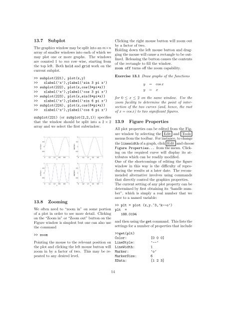
13.7 SubplotThe graphics window may be split into an m⇥narray of smaller windows into each of which wemay plot one or more graphs. The windowsare counted 1 to mn row–wise, starting fromthe top left. Both hold and grid work on thecurrent subplot.>> subplot(221), plot(x,y)>> xlabel(’x’),ylabel(’sin 3 pi x’)>> subplot(222), plot(x,cos(3*pi*x))>> xlabel(’x’),ylabel(’cos 3 pi x’)>> subplot(223), plot(x,sin(6*pi*x))>> xlabel(’x’),ylabel(’sin 6 pi x’)>> subplot(224), plot(x,cos(6*pi*x))>> xlabel(’x’),ylabel(’cos 6 pi x’)subplot(221) (or subplot(2,2,1)) specifiesthat the window should be split into a 2 ⇥ 2array and we select the first subwindow.13.8 ZoomingWe often need to “zoom in” on some portionof a plot in order to see more detail. Clickingon the “Zoom in” or “Zoom out” button on theFigure window is simplest but one can also usethe command>> zoomPointing the mouse to the relevant position onthe plot and clicking the left mouse button willzoom in by a factor of two. This may be repeatedto any desired level.Clicking the right mouse button will zoom outby a factor of two.Holding down the left mouse button and draggingthe mouse will cause a rectangle to be outlined.Releasing the button causes the contentsof the rectangle to fill the window.zoom off turns o↵ the zoom capability.Exercise 13.1 Draw graphs of the functionsy = cos xy = xfor 0 apple x apple 2 on the same window. Use thezoom facility to determine the point of intersectionof the two curves (and, hence, the rootof x = cos x) to two significant figures.13.9 Figure PropertiesAll plot properties can be edited from the Figurewindow by selecting the Edit and Toolsmenus from the toolbar. For instance, to changethe linewidth of a graph, click Edit and chooseFigure Properties... from the menu. Clickingon the required curve will display its attributeswhich can be readily modified.One of the shortcomings of editing the figurewindow in this way is the di culty of reproducingthe results at a later date. The recommendedalternative involves using commandsthat directly control the graphics properties.The current setting of any plot property can bedetermined by first obtaining its “handle number”,which is simply a real number that wesave to a named variable:>> plt = plot (x,y.^3,’k--o’)plt =188.0194and then using the get command. This lists thesettings for a number of properties that include>>get(plt)Color: [0 0 0]LineStyle: ’--’LineWidth: 1Marker:’o’MarkerSize: 6XData: [1 2 3]14