In order to plot this we have to decide on theranges of x and y—suppose 2 apple x apple 4 and1 apple y apple 3. This gives us a square in the (x, y)–plane. Next, we need to choose a grid on thisdomain; Figure 8 shows the grid with intervals0.5 in each direction. Finally, we have to eval-as corresponding to the (i, j)th entry in a matrix,then (X(i,j), Y(i,j)) are the coordinates of thepoint. We then need to evaluate the function f usingX and Y in place of x and y, respectively. Asin Example 14.1, elementwise operations (powers,products, etc.) are usually appropriate.Example 23.1 Plot the surface defined by the functionf(x, y) =(x 3) 2 (y 2) 2for 2 apple x apple 4 and 1 apple y apple 3.>> [X,Y] = meshgrid(2:.2:4, 1:.2:3);>> Z = (X-3).^2-(Y-2).^2;>> mesh(X,Y,Z)>> title(’Saddle’), xlabel(’x’),ylabel(’y’)Fig. 8: An example of a 2D griduate the function at each point of the grid and“plot” it.Suppose we choose a grid with intervals 0.5 ineach direction for illustration. The x– and y–coordinates of the grid lines arex = 2:0.5:4; y = 1:0.5:3;in Matlab notation. We construct the grid withmeshgrid:Fig. 9: Plot of Saddle function.>> [X,Y] = meshgrid(2:.5:4, 1:.5:3);>> XExercise 23.1 Repeat the previous example replacingmesh by surf and then by surfl. Consult theX =2.0000 2.5000 3.0000 3.5000 4.0000 help pages to find out more about these functions.2.0000 2.5000 3.0000 3.5000 4.0000Example 23.2 Plot the surface defined by the function2.0000 2.5000 3.0000 3.5000 4.00002.0000 2.5000 3.0000 3.5000 4.0000f = xye 2(x2 +y 2 )2.0000 2.5000 3.0000 3.5000 4.0000>> Yon the domain 2 apple x apple 2, 2 apple y apple 2. Find theY =1.0000 1.0000 1.0000 1.0000values and locations of the maxima and minima of1.0000 the function.1.5000 1.5000 1.5000 1.5000 1.50002.0000 2.0000 2.0000 2.0000 2.0000 >> [X,Y] = meshgrid(-2:.1:2,-2:.2:2);2.5000 2.5000 2.5000 2.5000 2.5000 >> f = -X.*Y.*exp(-2*(X.^2+Y.^2));3.0000 3.0000 3.0000 3.0000 3.0000 >> figure (1)If we think of the ith point along from the leftand the jth point up from the bottom of the grid)>> mesh(X,Y,f), xlabel(’x’), ylabel(’y’), grid>> figure (2), contour(X,Y,f)>> xlabel(’x’), ylabel(’y’), grid, hold on37
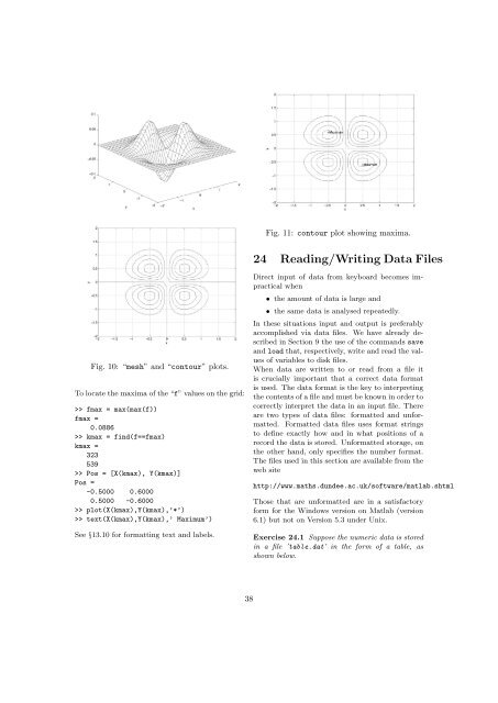
Fig. 11: contour plot showing maxima.24 Reading/Writing Data FilesFig. 10: “mesh” and “contour” plots.To locate the maxima of the “f” values on the grid:>> fmax = max(max(f))fmax =0.0886>> kmax = find(f==fmax)kmax =323539>> Pos = [X(kmax), Y(kmax)]Pos =-0.5000 0.60000.5000 -0.6000>> plot(X(kmax),Y(kmax),’*’)>> text(X(kmax),Y(kmax),’ Maximum’)See §13.10 for formatting text and labels.Direct input of data from keyboard becomes impracticalwhen• the amount of data is large and• the same data is analysed repeatedly.In these situations input and output is preferablyaccomplished via data files. We have already describedin Section 9 the use of the commands saveand load that, respectively, write and read the valuesof variables to disk files.When data are written to or read from a file itis crucially important that a correct data formatis used. The data format is the key to interpretingthe contents of a file and must be known in order tocorrectly interpret the data in an input file. Thereare two types of data files: formatted and unformatted.Formatted data files uses format stringsto define exactly how and in what positions of arecord the data is stored. Unformatted storage, onthe other hand, only specifies the number format.The files used in this section are available from theweb sitehttp://www.maths.dundee.ac.uk/software/matlab.shtmlThose that are unformatted are in a satisfactoryform for the Windows version on Matlab (version6.1) but not on Version 5.3 under Unix.Exercise 24.1 Suppose the numeric data is storedin a file ’table.dat’ in the form of a table, asshown below.38
- Page 1 and 2: An Introduction to MatlabVersion 3.
- Page 3 and 4: 1 MATLAB• Matlab is an interactiv
- Page 5: These are not allowable:Net-Cost, 2
- Page 8 and 9: Note that the components of x were
- Page 10 and 11: For example, if u = [10, 11, 12], v
- Page 12 and 13: a.*b -24, ans./cans =-18 -10 0 12 2
- Page 14 and 15: Colours Line Styles/symbolsy yellow
- Page 16 and 17: YData: [27 8 1]ZData:[1x0 double]Th
- Page 18 and 19: 14 Elementwise ExamplesExample 14.1
- Page 20 and 21: 0 00 0The second command illustrate
- Page 22 and 23: 9 10 11 1220 0 5 4>> J(1,1)ans =1>>
- Page 24 and 25: 15.12 Sparse MatricesMatlab has pow
- Page 26 and 27: It is well-known that the solution
- Page 28 and 29: the corresponding number, and two f
- Page 30 and 31: -2.0000 3.1416 5.0000-5.0000 -3.000
- Page 32 and 33: if logical test 1Commands to be exe
- Page 34 and 35: 6 8 0 1>> k = find(A==0)k =29Thus,
- Page 36 and 37: function [A] = area2(a,b,c)% Comput
- Page 40 and 41: 100 2256200 4564300 3653400 6798500
- Page 42 and 43: ’string’,’lin-log’,...’po
- Page 44 and 45: Matrix analysis.cond Matrix conditi
- Page 46 and 47: imag, 42inner product, 8, 21, 22int