MatlabNotes

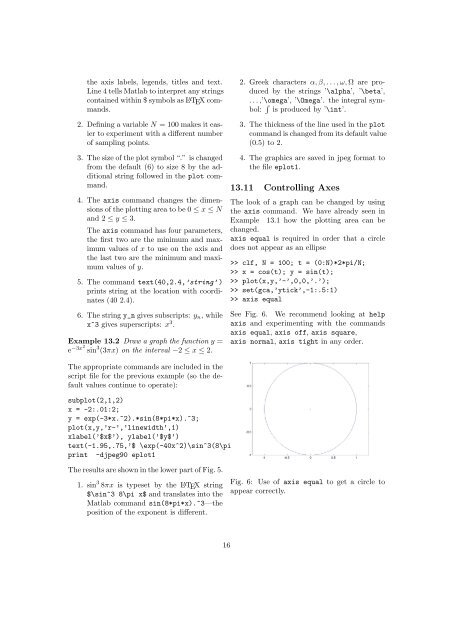
the axis labels, legends, titles and text.Line 4 tells Matlab to interpret any stringscontained within $ symbols as L A TEX commands.2. Defining a variable N = 100 makes it easierto experiment with a di↵erent numberof sampling points.3. The size of the plot symbol “.” is changedfrom the default (6) to size 8 by the additionalstring followed in the plot command.4. The axis command changes the dimensionsof the plotting area to be 0 apple x apple Nand 2 apple y apple 3.The axis command has four parameters,the first two are the minimum and maximumvalues of x to use on the axis andthe last two are the minimum and maximumvalues of y.5. The command text(40,2.4,’string’ )prints string at the location with coordinates(40 2.4).6. The string y_n gives subscripts: y n ,whilex^3 gives superscripts: x 3 .Example 13.2 Draw a graph the function y =e 3x2 sin 3 (3⇡x) on the interval 2 apple x apple 2.2. Greek characters ↵, ,...,!, ⌦ are producedby the strings ’\alpha’, ’\beta’,...,’\omega’, ’\Omega’. the integral symbol:R is produced by ’\int’.3. The thickness of the line used in the plotcommand is changed from its default value(0.5) to 2.4. The graphics are saved in jpeg format tothe file eplot1.13.11 Controlling AxesThe look of a graph can be changed by usingthe axis command. We have already seen inExample 13.1 how the plotting area can bechanged.axis equal is required in order that a circledoes not appear as an ellipse>> clf, N = 100; t = (0:N)*2*pi/N;>> x = cos(t); y = sin(t);>> plot(x,y,’-’,0,0,’.’);>> set(gca,’ytick’,-1:.5:1)>> axis equalSee Fig. 6. We recommend looking at helpaxis and experimenting with the commandsaxis equal, axis off, axis square,axis normal, axis tight in any order.The appropriate commands are included in thescript file for the previous example (so the defaultvalues continue to operate):subplot(2,1,2)x = -2:.01:2;y = exp(-3*x.^2).*sin(8*pi*x).^3;plot(x,y,’r-’,’linewidth’,1)xlabel(’$x$’), ylabel(’$y$’)text(-1.95,.75,’$ \exp(-40x^2)\sin^3(8\pi x)$’)print -djpeg90 eplot1The results are shown in the lower part of Fig. 5.1. sin 3 8⇡x is typeset by the L A TEX string$\sin^3 8\pi x$ and translates into theMatlab command sin(8*pi*x).^3—theposition of the exponent is di↵erent.Fig. 6: Use of axis equal to get a circle toappear correctly.16