Artistic Simulation of Curly Hair - Pixar Graphics Technologies

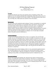
p'2d 1d 2dd43p'p'p'd 0p'5p1e 1p12p354e 0e e 42ep0p3p3 4Elastic rods model (E = G = 8 × 10 9 )Figure 3: Original curve (bold line) with points p i and edges e ioverlaid with corresponding smoothed curve (thin blue line) withpoints p ′ i and edges defined by vectors d i.Our bending model (k b = 3 × 10 4 , c b = 1.74 × 10 3 )Figure 2: Simple example of a perfect helical curl undergoingmotion from the walk cycle of Figure 12. The elastic rod model (top)introduces rotation around the helix, apparent in the orientation ofthe end of the curl, while our bending model (bottom) does not.of curls (Section 3.3). These three springs comprise our per hairforce model.3.1 Stretch SpringWe define our hair model using a set of particle positions connectedby linear springs. Let each hair be defined by a set of current particlepositions P = {p 0, . . . , p N−1} and initial rest pose particles,¯P , where ¯· denotes rest quantities. Let the current velocities forthese particles be V = {v 0, . . . , v N−1} and the polyline edgesconnecting hair particles be e i = p i+1 − p i. We compute a standarddamped linear spring force on particle i byf s(k s, c s) i = k s(‖ e i ‖ − ‖ ē i ‖)ê i + c s(∆v i · ê i)ê i (1)where k s are the spring and c s the damping coefficients, ∆v i =v i+1 − v i, ‖ · ‖ denotes vector length and ˆ· vector normalization.Because springs in our model are connecting two particles, eachof our spring forces is applied equally to both particles in oppositedirections.Our artists also want to enable bounce during a walk cycle, for example,by allowing hair to slightly stretch (see Figure 12 and thevideo for an example). To allow this artistic stretch of the hair withoutusing stiff springs, we impose an upper limit on the stretch ofthe polyline similar to the biased strain limiting approach presentedin [Selle et al. 2008]. During the spring damping calculation, werecurse from the root to the tip limiting the velocity of the hair particleif ∆vi2 exceeds a threshold. After we update positions, weagain recurse from the root of the hair to the tip shortening edgesthat exceed the specified stretch allowance. By using this limiter,artists are able to control the desired amount of stretch allowed bythe system.3.2 Bending SpringOur method to control bending is most similar to the elastic rodsmodel [Bergou et al. 2008; Bergou et al. 2010], which computesthe material frame as the minimizer of elastic energy of the curve.They use these material frames to compute the bending and twistingenergies along the rod. However, the formulation of Bergou et al.introduces rotation during simple motion of a curl, such as a walkcycle, shown in Figure 2 top. This rotation can be removed by! = 0 ! = 2 ! = 4 ! = 6 ! =∞Figure 4: Example of a stylized curly hair (far left) and thesmoothed curves (blue) computed with α at 2, 4, 6, and ∞.increasing the material’s stiffnesses, but this change leads to wirelikebehavior (see video).This type of rotation in the curl, while physically accurate, is undesirablefor our application. Our hair model instead introducesa method to stably generate the material frame by parallel transportingthe root frame of the hair along a smoothed piecewise linearcurve (see Section 3.2.1). The result of using our smoothedcurve is a series of frames that are not highly influenced by smallchanges in point positions, avoiding unwanted rotation as illustratedby Figure 2 bottom. Our bending formulation uses reference vectorsposed in the frames from the smoothed curve to compute thebending force (see Section 3.2.2).3.2.1 Smoothing FunctionLet Λ = {λ 0, . . . , λ N−1} be a set of N elements in R 3 associatedwith a hair, such as particle positions or velocities. We define oursmoothing function, d i = ς(Λ, α) i, with an infinite impulse response(IIR) Bessel filter (for examples, see [Najim 2006]). Thesefilters are recursive functions, combining the input and prior resultsto produce each new result.To compute the results, we take as input the smoothing amount,α ≥ 0, in units of length along the curve. Let β = min(1, 1 −exp(−l/α)) where l is the average rest length per segment of thehair being smoothed. We then recursively compute vectors d i ∀i ∈[0 . . . N − 2] with the equationd i = 2(1 − β)d i−1 − (1 − β) 2 d i−2 + β 2 (λ i+1 − λ i) . (2)By choosing these coefficients and initializing d −2 = d −1 = λ 1 −λ 0, this equation reduces to d 0 = λ 1 − λ 0 at i = 0. Subsequentd i values are weighted towards this initial direction, an importantproperty for our usage of this function.When Λ is a set of positions, we can reconstruct the smoothed polylineby recursively adding the vectors from the fixed root position.The new points, p ′ i ∀i ∈ [1 . . . N − 1], are defined byp ′ i = p ′ i−1 + d i−1 (3)where p ′ 0 = λ 0, the root of the polyline. We show the relationshipbetween an original and smoothed curve in Figure 3.