Freshwater Algae: Identification and Use as Bioindicators

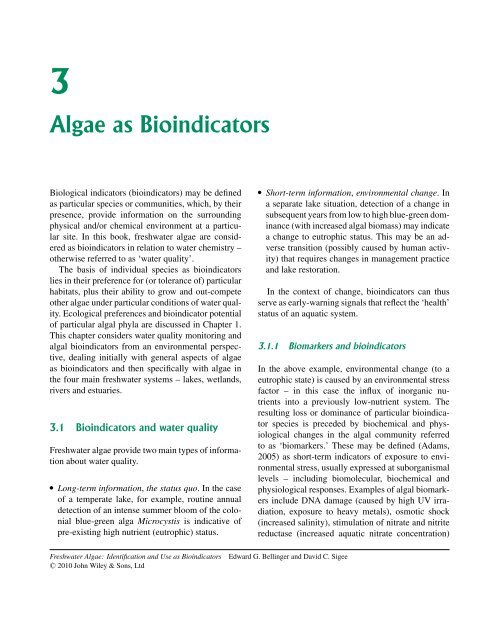
3Algae as BioindicatorsBiological indicators (bioindicators) may be definedas particular species or communities, which, by theirpresence, provide information on the surroundingphysical and/or chemical environment at a particularsite. In this book, freshwater algae are consideredas bioindicators in relation to water chemistry –otherwise referred to as ‘water quality’.The basis of individual species as bioindicatorslies in their preference for (or tolerance of) particularhabitats, plus their ability to grow and out-competeother algae under particular conditions of water quality.Ecological preferences and bioindicator potentialof particular algal phyla are discussed in Chapter 1.This chapter considers water quality monitoring andalgal bioindicators from an environmental perspective,dealing initially with general aspects of algaeas bioindicators and then specifically with algae inthe four main freshwater systems – lakes, wetlands,rivers and estuaries.3.1 Bioindicators and water qualityFreshwater algae provide two main types of informationabout water quality. Long-term information, the status quo. In the caseof a temperate lake, for example, routine annualdetection of an intense summer bloom of the colonialblue-green alga Microcystis is indicative ofpre-existing high nutrient (eutrophic) status. Short-term information, environmental change. Ina separate lake situation, detection of a change insubsequent years from low to high blue-green dominance(with increased algal biomass) may indicatea change to eutrophic status. This may be an adversetransition (possibly caused by human activity)that requires changes in management practiceand lake restoration.In the context of change, bioindicators can thusserve as early-warning signals that reflect the ‘health’status of an aquatic system.3.1.1 Biomarkers and bioindicatorsIn the above example, environmental change (to aeutrophic state) is caused by an environmental stressfactor – in this case the influx of inorganic nutrientsinto a previously low-nutrient system. Theresulting loss or dominance of particular bioindicatorspecies is preceded by biochemical and physiologicalchanges in the algal community referredto as ‘biomarkers.’ These may be defined (Adams,2005) as short-term indicators of exposure to environmentalstress, usually expressed at suborganismallevels – including biomolecular, biochemical andphysiological responses. Examples of algal biomarkersinclude DNA damage (caused by high UV irradiation,exposure to heavy metals), osmotic shock(increased salinity), stimulation of nitrate and nitritereductase (increased aquatic nitrate concentration)Freshwater Algae: Identification and Use as BioindicatorsC○ 2010 John Wiley & Sons, LtdEdward G. Bellinger and David C. Sigee

100 3 ALGAE AS BIOINDICATORSBIOMARKERSENVIRONMENTALMONITORINGBIOINDICATORSPECIESCompetitionsuccessReproductionGrowthweeks-yearsPhysiologicalBioenergeticsdays-weeksFigure 3.1 Hierarchical responsesof algae to environmental change,such as alterations in water quality.The time-response changes relateto sub-organismal (left), individual(middle) and population (right)aspects of the algal community. Environmentalmonitoring of the algalresponse can be carried out atthe biomarker or bioindicator specieslevel. Adapted from Adams (2005).BiochemicalBiomolecularENVIRONMENTALCHANGEseconds-daysand stimulation of phosphate transporters/reductionin alkaline phosphatase secretion (increased aquaticinorganic phosphate concentration).The time scale of perturbations in the algal communitythat results from environmental change (stress)can be expressed as a flow diagram (Fig. 3.1), withmonitoring of algal response being carried out eitherat the biomarker or bioindicator species level. Althoughthe rapid response of biomarkers potentiallyprovides an early warning system for monitoring environmentalchange (e.g. in water quality), the use ofbioindicators has a number of advantages (Table 3.1)including high ecological relevance and the ability toanalyse environmental samples (chemically-fixed) atany time after collection.3.1.2 Characteristics of bioindicatorsThe potential for freshwater organisms to reflectchanges in environmental conditions was first notedby Kolenati (1848) and Cohn (1853), who observedthat biota in polluted waters were different fromthose in non-polluted situations (quoted in Liebmann,1962).Since that time much detailed information hasaccumulated about the restrictions of different organisms(e.g. benthic macroinvertebrates, planktonicalgae, fishes, macrophytes) to particular types ofaquatic environment, and their potential to act as environmentalmonitors or bioindicators. Knowledge offreshwater algae that respond rapidly and predictably

3.1 BIOINDICATORS AND WATER QUALITY 101Table 3.1ChangeMain Features of Biomarkers and Bioindicators in the Assessment of EnvironmentalMajor Features Biomarkers BioindicatorsTypes of response Subcellular, cellular Individual-communityPrimary indicator of Exposure EffectsSensitivity to stressors High LowRelationship to cause High LowResponse variability High LowSpecificity to stressors Moderate-high Low-moderateTimescale of response Short LongEcological relevance Low HighAnalysis requirement Immediate, on site Any time after collection (fixed sample)Adapted from Adams, 2005.to environmental change has been particularly useful,with the identification of particular indicator speciesor combinations of species being widely used in assessingwater quality.Single speciesIn general, a good indicator species should have thefollowing characteristics: a narrow ecological range rapid response to environmental change well defined taxonomy reliable identification, using routine laboratoryequipment wide geographic distribution.Combinations of speciesIn almost all ecological situations it is the combinationof different indicator species or groups that isused to characterize water quality. Analysis of all orpart of the algal community is the basis for multivariateanalysis (Section 3.4.3), application of bioindices(Sections 3.2.2 and 3.4.4) and use of phytopigmentsas diagnostic markers (Section 3.5.2)3.1.3 Biological monitoring versus chemicalmeasurementsIn terms of chemistry, water quality includes inorganicnutrients (particularly phosphates and nitrates),organic pollutants (e.g. pesticides), inorganic pollutants(e.g. heavy metals), acidity and salinity. In anideal world, these would be measured routinely in allwater bodies being monitored, but constraints of costand time have led to the widespread application ofbiological monitoring.The advantages of biological monitoring over separatephysicochemical measurements to assess waterquality are that it: reflects overall water quality, integrating the effectsof different stress factors over time; physicochemicalmeasurements provide information on one pointin time. gives a direct measure of the ecological impactof environmental parameters on the aquaticorganisms. provides a rapid, reliable and relatively inexpensiveway to record environmental conditions across anumber of sites.Biological monitoring has been particularly useful,for example, in implementing the European

102 3 ALGAE AS BIOINDICATORSTable 3.2Trophic Classification of Temperate Freshwater Lakes, Based on a Fixed Boundary SystemTrophic CategoryUltraoligotrophic Oligotrophic Mesotrophic Eutrophic HypertrophicNutrient concentration (µgl −1 )Total phosphorus (mean annual value) 100Orthophosphate a 100DIN a 100Chlorophyll a concentration (µgl −1 )Mean concentration in surface waters 25Maximum concentration in surface waters 75Total volume of planktonic algae b 0.12 0.4 0.6–1.5 2.5–5 >5Secchi depth (m)Mean annual value >12 12–6 6–3 3–1.5 6 >3.0 3–1.5 1.5–0.7

Table 3.3 Lake Trophic Status: Phytoplankton Succession and Algal BioindicatorsLake Type Spring Summer Autumn Mid-Summer Algal Bioindicators ExampleOligotrophicDIATOMSCyclotella DINO CeratiumBG GomphosphaeriaDIA Cyclotella comensisRhizosolenia spp.G Staurodesmus spp.CarinthianLakes 1Wastwater 2EnnerdaleMesotrophicDIATOMS CHRYSO DINO DIATOMSAsterionella Mallomonas Ceratium AsterionellaBG GomphosphaeriaGREEN SphaerocystisDIA Tabellaria flocculosaCHR Dinobryon divergens, MallomonascaudataG Sphaerocystis schroeteri,Dictyosphaerium elegans,Cosmarium spp, Staurastrum sppDINO Ceratium hirundinellaBG Gomphosphaeria spp.LunzerUntersee 1Bodensee 3Erken 4Windermere 2GrasmereEutrophicDIATOMS GREEN BG DINO DIATOMSAsterionella Eudorina Anabaena Ceratium Steph.CRYPT Aphan. BGCryptomonas MicrocystisDIA Aulacoseira spp., StephanodiscusrotulaG Eudorina spp., Pandorina morum,Volvox spp.BG Anabaena spp., Aphanizomenon flosaquae,Microcystis aeruginosaPrairie Lakes 5Norfolk Broad 2RostherneMere 2HypertrophicSMALL DIATOMS GREEN GREEN BGSteph. Scenedesmus Pediaastrum AphanocapsaDIA Stephanodiscus hantzschiiG Scenedesmus spp., Ankistrodesmusspp., Pediastrum spp.BG Aphanocapsa spp., Aphanothece spp,Synechococcus spp.Fertilisedwaterse.g. Třeboňfishponds 6Abbreviations: Main phytoplankton groups: BG, blue-green algae; Chryso, chrysophytes; Crypt, cryptomonads; Dino, dinoflagellates.Genera: Steph., Stephanodiscus; Aphan., Aphanizomenon.Location of lakes: 1 Austria, 2 UK, 3 Germany, 4 Sweden, 5 USA, 6 Czech Republic.Table adapted from Sigee (2004), originally from Reynolds (1990).

104 3 ALGAE AS BIOINDICATORSLocal direct and diffuse loadfrom forestry activitiesALocal acid surfaceand groiund waterdischarges (rockyand sandy soils)Local and diffuseload from wetlandsPELAGICZONEBIndustrial effluentsCLITTORALZONEEffects and mixingof inflowing watersDiffuse load fromvillagesLocal direct and diffuse load from agricultureLocal and diffuseload from trafficFigure 3.2Lake water quality: phytoplankton and periphyton as bioindicators. General lake water quality: phytoplanktonin pelagic zone (° sites A, B, C). Local water quality at edge of lake ( • periphyton in littoral zone), with inputs(→) from a range of surrounding terrestrial sources. Figure adapted and redrawn from Eloranta, 2000. Suitability of water for human use. This includescompliance of water quality with regulations forhuman consumption and recreation. Build-upof colonial blue-green algal populations, withincreased concentrations of algal toxins, can leadto closure of lakes for production of drinking waterand recreation. The use of a reactive monitoringprogramme for blue-green algal development overthe summer months is now an essential part ofwater management for in many aquatic systems(e.g. Hollingworth Lake, United Kingdom – Sigee,2004). Conservation assessment. Analysis of freshwateralgae has become an important part of the surveyand data collection programme used in the evaluationof lakes for their nature conservation value(Duker and Palmer, 2009). Evaluation of water

106 3 ALGAE AS BIOINDICATORSDirective (WFD: European Union, 2000), which requiresMember States to monitor the ecology of waterbodies to achieve ‘good ecological status’. Macrophytesand attached algae together form one ‘biologicalelement’ that needs to be assessed underthis environmental programme (see also ‘multiproxyapproach’ – Section 3.2.2).Local water quality Various authors have analysedbenthic or epiphytic algal populations in relationto water quality, including the extensive periphytongrowths that occur in the littoral region of many lakes.These algae are particularly useful in relation to localwater conditions (e.g. localized accumulations ofmetal toxins, point source and diffuse loading at theedge of the lake), since their permanent location atparticular sites gives a high degree of spatial resolutionwithin the water body.Localized metal accumulations Cattaneo et al.(1995) studied periphyton growing epiphytically inmacrophyte beds of a fluvial lake in the St LawrenceRiver (Canada), to see if they could resolve periphytoncommunities in relation to water quality (toxicand non-toxic levels of mercury) under differing ecologicalconditions (e.g. fine versus coarse sediment).The periphyton, composed of green algae (40%),blue-greens (25%) diatoms (25%) and other phyla,was collected from various sites and analysed in termsof taxonomic composition and size profile. Multivariate(cluster and biotic index) analysis of periphytoncommunities gave greatest separation in relationto physical ecological (particularly substrate)conditions rather than water quality. The authors recommendedthat the use of benthic algae as aquaticbioindicators should involve sampling from similarsubstrate sites to eliminate ecological variation otherthan water quality.Point source and diffuse loading at the edge ofthe lake Water quality in the littoral zone may differconsiderably from that in the main part of the lake.This is partly due to the proximity of the terrestrialecosystem (with inflow from the surrounding catchmentarea) and partly due to the distinctive zone oflittoral macrophyte vegetation, making an importantbuffer zone between the shore and open water (Eloranta,2000). Analysis of littoral algae, either by multivariateanalysis or determination of bioindices, hasthe potential to provide information on water qualityat particular sites along the edge of the lake in relationto point discharges (stream inflows, industrialand sewage discharges) and diffuse loadings. The latterinclude input from surrounding agricultural land,discharges from domestic areas, traffic pollutants andloading from local ecosystems such as forests andpeat bogs (Eloranta, 2000) – Fig. 3.2.Sampling and analysis of littoral algae Althoughattached algal communities (as with phytoplankton)can theoretically be related to water qualityin terms of total biomass, this does not correlate wellwith nutrient loading (King et al., 2006) – chieflydue to grazing and (in eutrophic waters) competitionwith phytoplankton. Also, nutrients in the water canbe supplemented by nutrients arising from the substratum.Species counts, on the other hand, can provide auseful measure of water quality. Recent recommendationsfor littoral sampling (King et al., 2006: see alsoSection 2.10) concentrate particularly on diatoms –collecting specimens from stones and macrophytes(Fig. 2.29), since these substrata are particularly commonat the edge of lakes. Epipelic diatoms (present onmud and silt) are probably less useful as bioindicatorssince they are particularly liable to respond to substrate‘pore-water’ chemistry rather than general waterquality. The epipelic diatom community of manylowland lakes also tends to be dominated by Fragilariaspecies, which take advantage of favourablelight conditions in the shallow waters, but are poorindicators of water quality – having wide tolerance tonutrient concentrations. Having obtained samples andcarried out species counts of diatoms from habitatswithin the defined littoral sampling area, weightedaverageindices can be calculated as with river diatoms(Section 3.4.5/6) and related to water quality.3.2.2 Fossil algae as bioindicators: lakesediment analysisRecent water legislation, including the US CleanWater Act (Barbour et al., 2000) and the EuropeanCouncil Water Framework Directive (WFD: EuropeanUnion, 2000) have required the need to assesscurrent water status in relation to some baselinestate in the past. This baseline state (referred to as

3.2 LAKES 107‘reference conditions’) defines an earlier situationwhen there was no significant anthropogenic influenceon the water body. In the United Kingdom, thisreference baseline is generally set at about 1850,prior to the modern era of industrialization and agriculturalintensification. Having defined the referenceconditions, contemporary analyses can then be usedto make a comparative assessment of human influenceson lake biology, hydromorphology and waterchemistry. For a particular water body, the absenceof long-term contemporary data means that referenceconditions have to be assessed on a retrospective basis,including the use of palaeolimnology – the studyof the lake sediment record. The use of lake sedimentsto generate a historical record only gives reliableresults under conditions of optimal algal preservation(see below) and if the sediments are undisturbed bywind, bottom-feeding fish and invertebrates.Lake sediments – algal accumulation andpreservationContinuous sedimentation of phytoplankton from thesurface waters (euphotic zone) of lakes leads to thebuild-up of sediment, with the accumulation of bothplanktonic and benthic algal remains at the bottom ofthe water column. In a highly productive lake such asRostherne Mere, United Kingdom (Fig. 3.5), the wetsedimentation rate in the deepest parts of the waterbody has been estimated at 20 mm year −1 (Prartanoand Wolff, 1998), with subsequent compression asfurther sedimentation and decomposition occurs. Decompositionof algal remains leads to the loss of mostorganic biomass, and algal identification is largelybased on the relatively resistant inorganic (siliceous)components of diatoms and chrysophytes (Section1.9). Optimal preservation of this cell wall materialrequires anaerobic conditions, and sediment samplesare best taken from central deep parts of the lakerather than from shallow regions such as the littoralzone (Livingstone, 1984).Diatom bioindicators within sedimentsWithin lake sediments, diatoms have been particularlyuseful as bioindicators (Section 1.10) of pastlake acidification (Battarbee et al., 1999), pointsources of eutrophication (Anderson et al., 1990)and total phosphorus concentration (Hall and Smol,1999). The widespread use of lake sediment diatomsfor reconstruction of past water quality is supportedby the European Diatom Database Initiative (EDDI).This web-based information system is designed toenhance the application of diatom analysis to problemsof surface water acidification, eutrophicationand climate change. The EDDI has been producedby combining and harmonizing data from a series ofsmaller datasets from around Europe and includes adiatom slide archive, electronic images of diatoms,new training sets for environmental reconstruction(see below) and applications software for manipulatingdata. In addition to the EDDI, other databases arealso available – including a large-scale database forbenthic diatoms (Gosselain et al., 2005).Diatoms within sediments are chemically cleanedto reveal frustule structure (Section 2.5.4), identifiedand species counts expressed as percentage total. Numerousexamples of cleaned diatom images from lakesediments are shown in Chapter 4. As with fossilchrysophytes (Section 1.9), subsequent analysis ofdiatom species counts to provide information on waterquality can involve the use of transfer functions,species assemblages and may be part of a multiproxyapproach. The data obtained, coupled with radiometricdating of sediment cores, provide information ontimes and rates of change and help in setting targetsfor specific restoration procedures to be carried out.Transfer functions Transfer functions are mathematicalmodels that allow contemporary data to beapplied to fossil diatom assemblages for the quantitativereconstruction of (otherwise unknown) past waterquality. Various authors (Bennion et al., 2004; Tayloret al., 2006; Bennion and Battarbee, 2007) have describedthe use of this approach, which is as follows. Generation of a predictive equation (transfer function)from a large number of lakes, in each caserelating the dataset of modern surface-sediment diatomssamples to lake water quality data (Bennionet al., 1996). The ‘training set’ of lakes shouldmatch the lake under study in terms of geographicregion and lake morphology, and should have arange of water quality characteristics extending

3.2 LAKES 109sites (Fig. 3.3 A, B, C), which indicated clear alterationsin water quality. In a number of deep lochs(C), limited eutrophication has occurred, with transitionfrom a Cyclotella/Achnanthes assemblage to aspecies combination (Asterionella/Aulacoseira) typicalof mesotrophic waters. Some shallow lochs (B)also showed nutrient increase, indicated by transitionfrom a non-planktonic (largely benthic) to a planktondominateddiatom population. In other cases, deepoligotrophic (E) and shallow (D) lochs showed littlechange in diatom assemblage, indicating minimalalteration in water quality.Multiproxy approach In a multiproxy approach,diatoms are just one of a number of groupsof organisms that are counted and analysed withinthe lake sediments (Bennion and Battarbee, 2007).For European limnologists, the stimulus for a multiproxyapproach has come with the most recent WaterFramework Directive (WFD; European Union,2000). This focuses on ecological integrity rather thansimply chemical water quality, for which the use ofhydro-chemical transfer functions and diatom speciesassemblage analysis are not sufficient.Multiproxy analysis uses as broad a range of organismswithin the food web (e.g. pelagic food web)as possible, commensurate with those biota with remainsthat persist in the sediment in an identifiableform. In addition to micro-algae (diatoms, chrysophytes),fossil indicators also include macroalgae(Charophyta), protozoa (thecamoebae), higher plants(pollen and macro-remains), invertebrates (chironomids,ostracods, cladocerans) and vertebrates (fishscales).This approach is illustrated by the study of Davidsonet al. (2005) on Groby Pool, United Kingdom,a shallow lake that has undergone nutrientenrichment in the past 200 years. Comparison of20-year slices from the sediment surface (recent:1980–2000) and base (reference: 1700–1720) indicatemajor changes in lake ecology (Fig. 3.4),driven primarily by alterations in water quality (Bennionand Battarbee, 2007). The ecological referencestate is one of dominance by benthic diatoms,colonization by low nutrient-adapted macro-algaeand higher plants, with detectable invertebrates restrictedto plant-associated Chydoridae. In contrastto this, the current-day ecosystem is much moreproductive – dominated by planktonic algae, highTOPPlanktonicStephanodiscusEpiphytic:CocconeisHigher plants:PotamogetonCallitricheNymphoeaZooplankton:CeriodaphniaBosminaDaphniaDominantdiatomsMacroalgae andhigher plantsInvertebratesBOTTOMBenthicFragilaria spp.Charophyta:Nitella, CharaHigher plants:Myriophyllum,UtriculariaPlant-associatedChydoridFigure 3.4 Multi-proxy palaeoecological analysis of a sediment core: Groby Pool, United Kingdom. Analysis of20-year slices from the top (recent ecology, ∼1980–2000) and bottom (reference ecology, ∼1700–1720) samples of thecore. Figure adapted and redrawn from Bennion and Battarbee (2007), original data from Davidson et al. (2005).

110 3 ALGAE AS BIOINDICATORSnutrient-adapted macrophytes and abundant zooplanktonpopulations.Other examples of a multiproxy approach to lakesediment analysis include the studies of Cattaneoet al. (1998) on heavy metal pollution in Italian Laked’Orta (Section 3.2.2) and studies on eutrophicationin six Irish lakes (Taylor et al., 2006). The latter studyinvolved sediment analysis of cladocerans, diatomsand pollen from mesotrophic-hypertrophic lakes, toreconstruct past variations in water quality and catchmentconditions over the past 200 years. The resultsshowed that five of the lakes were in a far more productivestate compared to the beginning of the sedimentrecord, with accelerated enrichment since 1980.3.2.3 Water quality parameters: inorganic andorganic nutrients, acidity and heavymetalsA wide range of chemical parameters can beconsidered in relation to general lake water quality– including total salt content (conductivity), inorganicnutrients (nitrogen and phosphorus), solubleorganic nutrients, acidity, heavy metal contaminationand presence of coloured matter (causedparticularly by humic materials). The diversity andinter-relationships of different lakes in relation tothese characteristics was emphasized by the studyof Rosen (1981), evaluating lake types and relatedplanktonic algae from August sampling of 1250Swedish standing waters. A summary from this studyof algae characteristic of Swedish acidified lakes,oligotrophic forest lakes (varying in phosphoruscontent and conductivity), humic lakes, mesotrophicand eutrophic lakes is given by Willen (2000).In this section, the role of algae as bioindicatorsis considered in reference to four main aspectsof lake water quality – inorganic nutrients,soluble organic nutrients, acidity and heavy metalcontamination.Inorganic nutrient status: oligotrophic toeutrophic lakesThe trophic classification of lakes, based primarilyon inorganic nutrient status, has become the majordescriptor of different lake types. Its importance reflects: the key role that nutrients have on the productivity,diversity and identity of algae and other lakeorganisms a major distinction between deep mountain lakes(typically oligotrophic) and shallow lowland lakes(typically eutrophic) the major impact that humans have on changingthe ecology of lakes, typically from oligotrophic toeutrophic ecological problems that may arise as lakes changefrom eutrophic to hypertrophic, leading to degenerativechanges that can only be reversed by humanintervention.The diverse ecological effects that increasing nutrientconcentrations have on lake ecology have beenwidely reported (e.g. Kalff, 2002; Sigee, 2004), includingthe ecological destabilization that occurs atvery high nutrient concentrations.Definition of terms Lake classification, fromoligotrophic (low nutrient) to mesotrophic and eutrophic(high nutrient), is based on the twin criteriaof productivity and inorganic nutrient concentration– particularly nitrates and phosphates. Variousschemes have been proposed to define these terms,including one developed by the Organization forEconomic Cooperation and Development (OECD,1982). This scheme (Table 3.2) uses fixed boundaryvalues for nutrient concentration (mean annualconcentration of total phosphorus), and productivity(chlorophyll-a concentration, Secchi depth). In thisscheme, for example, the mean annual concentrationof total phosphorus ranges from 4–10 µgl −1 foroligotrophic lakes, and 35–100 µgl −1 for eutrophicwaters. In addition to total phosphorus, boundariesfor the main soluble inorganic nutrients – orthophosphateand dissolved inorganic nitrogen (nitrate, nitrite,ammonia) have also been designated (TechnicalStandard Publication, 1982).

3.2 LAKES 111Phytoplankton net production (biomass) is determinedeither as chlorophyll-a concentration(mean/maximum annual concentration in surface waters)or as Secchi depth (mean/maximum annualvalue). Examples of total volumes of planktonic algaeat different trophic levels (Norwegian lakes) arealso given in Table 3.2, together with characteristicbioindicator algae.Algae as bioindicators of inorganic trophicstatusPlanktonic algae within lake surface (epilimnion)samples can be used to define lake trophic status interms of their overall productivity (Table 3.2) andspecies composition (Table 3.3). Species compositioncan be related to trophic status in four mainways – seasonal succession, biodiversity, bioindicatorspecies and determination of bioindices.1. Seasonal succession. In temperate lakes, thedevelopment of algal biomass and the sequence ofphytoplankton populations (seasonal succession) directlyrelate to nutrient availability. In all cases theseason commences with a diatom bloom, but subsequentprogression (Reynolds, 1990) can be separatedinto four main categories (Table 3.3). Oligotrophic lakes. In low nutrient lakes the springdiatom bloom is prolonged, and diatoms may dominatefor the whole growth period. Chrysophytes(Uroglena) and desmids (Staurastrum) may alsobe present, and in some lakes Ceratium and Gomphosphaeriamay be able to grow in the nutrientdepletedwaters by migrating down the water columnto higher nutrient conditions. Mesotrophic lakes. These have a shorter diatombloom (dominated by Asterionella), often followedby a chrysophyte phase then mid-summer dinoflagellate,blue-green and green algal blooms. Eutrophic lakes. In high nutrient lakes, the springdiatom bloom is further limited, leading to a clearwaterphase (dominated by unicellular algae), followedby a mid-summer bloom in which largeunicellular (Ceratium), colonial filamentous (Anabaena)and globular (Microcystis) blue-greenspredominate. Hypertrophic lakes. These include artificially fertilizedfish ponds (Pechar et al., 2002) and lakes withsewage discharges, and are dominated throughoutthe season by small unicellular algae withshort life cycles. The algae form a successionof dense populations, out-competing larger colonialorganisms which are unable to establishthemselves.2. Species diversity. Bioindices of species diversitycan be derived from species counts and fall intothree main categories (Sigee, 2004) – species richness(Margalef index), species evenness/dominance(Pielou index, Simpson index) and a combination ofrichness and dominance (Shannon–Wiener index).One of the most commonly-used indices (d), developedby Margalef (1958), combines data on the totalnumber of species identified (S) and total number ofindividuals (N), where:d = (S − 1)/ log e N (3.1)During the summer growth phase, species diversityis typically low in oligotrophic lakes, rising progressivelyin mesotrophic and eutrophic lakes, but fallingagain in some eutrophic/hypertrophic lakes wheresmall numbers of species may out-compete other algae.The effects of increasing nutrient levels on algaldiversity (d) are illustrated by Reynolds (1990),with summer-growth values of 3–6 for the nutrientdeficientNorth Basin of Lake Windermere (UnitedKingdom) – falling to levels of 2–4 in a nutrientrichlake (Crose Mere, United Kingdom) and 0.2–2for a hypertrophic water body (fertilized enclosure,Blelham Tarn, United Kingdom).3. Bioindicator species. Some algal species andtaxonomic groups show clear preferences for particularlake conditions, and can this act as potentialbioindicators. In a broad comparison of oligotrophicversus eutrophic waters, desmids (green algae) tendto occur mainly in low nutrient waters while colonial

112 3 ALGAE AS BIOINDICATORSblue-green algae are more typical of eutrophic waters.Such generalizations are not absolute, however, sincesome desmids (e.g. Cosmarium meneghinii, Staurastrumspp.) are typical of meso- and eutrophic lakes,while colonial blue-green algae such as Gomphosphaeriaare also found in oligotrophic waters.Although it is not possible to pin-point individualalgal species in relation to particular trophic states, itis possible to list organisms that are typical of summergrowths in different standing waters (Table 3.3).Identification of such indicator species, particularlyat high population levels, gives a good qualitativeindication of nutrient state. As an example of thisthe high-nutrient lake illustrated in Fig. 3.5 is characteristicof temperate eutrophic water bodies,with highproductivity, characteristic seasonal progression (Fig.2.8) and with the eutrophic bioindicator algae listed inTable 3.3. In addition to phytoplankton bioindicators,the trophic status of the lake is also reflected in extensivegrowths of attached algae such as CladophoraFigure 3.5 Eutrophic lake (Rostherne Mere, UnitedKingdom). The high nutrient status of the lake is indicatedby water analyses (mean annual total phosphorus>50 µgl −1 ), high productivity (maximum chlaconcentration typically >60 µgl −1 ) and characteristicbioindicator algae. These include planktonic blooms ofAnabaena, Aphanizomenon, Microcystis (colonial bluegreens)plus various eutrophic algae (see text). Attachedmacroalgae (Cladophora) and periphyton communities(present on the fringing reed beds Fig. 2.29) are alsowell-developed.(Fig. 2.28) and in the dense periphyton communities(Fig. 2.29) that occur in the littoral reed beds.Analysis of lake sediments (Capstick, unpublishedobservations) indicates increased eutrophication inrecent historical times, with higher proportions ofthe diatoms Asterionella formosa plus Aulacoseiragranulata var. angustissima and marked decreases inCyclotella ocellata and Tabellaria flocculosa (moretypical of low-nutrient waters) over the last 50 years.Although individual algal species can be rated primarilyin terms of trophic preferences, they are alsofrequently adapted to other related ecological factors. Acidity: oligotrophic waters are frequently slightlyacid with low Ca concentrations, and vice versa foreutrophic conditions. Nutrient balance: mesotrophic waters may benitrogen-limiting (high P/N ratio), promoting thegrowth of nitrogen-fixing (e.g. Anabaena) but notnon-fixing (e.g Oscillatoria) colonial blue-greenalgae. Long-term stability: In hypertrophic waters, dominationby particular algal groups may vary with thelong-term stability of the water body. High-nutrientlakes, with established populations of blue-greensand dinoflagellates, often have these as dominantalgae during the summer months. Small newlyformedponds, however, are often dominated byrapidly-growing chlorococcales (green algae) andeuglenoids. The latter are particularly prominent athigh levels of soluble organics (e.g. sewage ponds),using ammonium as a nitrogen source. Some of themost hypertrophic and ecologically-unstable watersare represented by artificially fertilized fishponds, such as those of the Třeboň wetlands, CzechRepublic (Pokorny et al., 2002a,b).In addition to considering individual algal species,taxonomic grouping (assemblages) may also beuseful environmental indicators. Reynolds (1980)considered species assemblages in relation to seasonalchanges and trophic status, with some groupings(e.g. Cyclotella comensis/Rhizosolenia) typicalof oligotrophic waters and others typical of eutrophic(e.g. Anabaena/Aphanizomeno/Gloeotrichia)

3.2 LAKES 113and hypertrophic (Pediastrum/Coelastrum/Oocystis)states. Consideration of algae as groups rather thanindividual species leads on to quantitative analysisand determination of trophic indices.4. Phytoplankton trophic indices. In mixed phytoplanktonsamples, algal counts can be quantitativelyexpressed as biotic indices to characterize laketrophic status (Willen, 2000). These indices occur atthree levels of complexity (Table 3.4).1. Indices based on major taxonomic groups Earlyphytoplankton indices, developed by Thunmark(1945), Nygaard (1949) and Stockner (1972) usedmajor taxonomic groups that were considered typicalof oligotrophic (particularly desmids) or eutrophic(chlorococcales, blue-greens, euglenoids) conditions.The proportions of eutrophic/oligotrophic speciesgenerated a simple ratio which could be used to designatetrophic status (Table 3.4a). Using the chlorophyceanindex of Thunmark (1945), for example,counts of chlorococcalean and desmid species canbe expressed as a ratio, which indicates trophic statusover the range oligotrophy (1).Although such indices provided useful information(see below), they tended to lack environmentalresolution since many algal classes turn out to be heterogeneous– containing species typical of oligo- andeutrophic lakes. Problems were also encountered insome of the early studies with sampling procedures,Table 3.4Lake Trophic IndicesIndex Calculation Result Reference(a) Major taxonomic groups: numbers of speciesChlorophycean index Chlorococcales spp./Desmidiales spp. 1 = eutrophyMyxophycean index Cyanophyta spp./Desmidiales 1 = eutrophyDiatom indexCentrales spp./PennalesEuglenophycean index Euglenophyta/Cyanophyta + ChlorophytaA/C diatom index Araphid pennate/centric diatom spp. 2 = eutrophy

114 3 ALGAE AS BIOINDICATORSDepth in Core (cm)05101520250.1 0.2 0.3 0.4 0.5 0.6 0.1A/C Ratio19801960184517001500Year (A.D.)Figure 3.6 Changes in the ratio of araphid pennate tocentric diatoms (A/C ratio) as an indicator of gradualeutrophication in Lake Tahoe (United States). The dramaticincrease in the A/C ratio during the late 1950s isassociated with increasing human population around thelake. Taken from Sigee (2004), adapted and redrawnfrom Byron and Eloranta, 1984.where net collection of algae resulted in loss of smallsized(single cells or small colonies) species. Suchalgae are often dominating elements in the planktoncommunity, and their loss from the sample meant thatthe index was not representative.Example: The A/C diatom index of Stockner(1972). The ratio of araphid pennate/centric diatoms(A/C ratio) provides a good example of the successfuluse of a broad taxonomic index in a particular lakesituation. Studies by Byron and Eloranta (1984) onthe sediments of Lake Tahoe (United States) showeda clear change in the diatom community during thelate 1950s (Fig. 3.6), consistent with eutrophication.The increase in A/C ratio (2. Thecorresponding ratio for oligotrophic indicators was0.7. The trophic state of lakes was calculated as theratio of eutrophic/oligotrophic species counts or asbiovolumes. Index values

3.2 LAKES 115Table 3.5 Organic Pollution: Most Tolerant Algal Genera and Species (Palmer, 1969)No. Taxon ClassPollutionIndexFreshwater HabitatGenus1 Euglena Eu 5 Planktonic2 Oscillatoria Cy 5 Planktonic or benthic3 Chlamydomonas Ch 4 Planktonic4 Scenedesmus Ch 4 Planktonic5 Chlorella Ch 3 Planktonic6 Nitzschia Ba 3 Benthic or planktonic7 Navicula Ba 3 Benthic8 Stigeoclonium Ch 2 Attached9 Synedra Ba 2 Planktonic and epiphyticspecies10 Ankistrodesmus Ch 2 PlanktonicSpecies1 Euglena viridis Eu 6 Ponds and shallow lakes2 Nitzschia palea Ba 5 Lakes and rivers3 Oscillatoria limosa Cy 4 Stagnant or standing waters4 Scenedesmus quadricauda Ch 4 Lake phytoplankton5 Oscillatoria tenuis Cy 4 Ponds and shallow pools6 Stigeoclonium tenue Ch 3 Epiphyte, shallow waters7 Synedra ulna Ba 3 Lake phytoplankton8 Ankistrodesmus falcatus Ch 3 Lake phytoplankton9 Pandorina morum Ch 3 Lake phytoplankton10 Oscillatoria chlorina Cy 2 Stagnant or standing watersTen most tolerant algal genera and species. listed (Palmer, 1969) in order of decreasing tolerance. Algalphyla: Cyanophyta (Cy), Chlorophyta (Ch), Euglenophyta (Eu) and Bacillariophyta (Ba).Pollution index – see text.pollution was originally pioneered by Kolkwitz andMarsson (1908).Palmer (1969) carried out an extensive literaturesurvey to assess the tolerance of algal species to organicpollution, and to incorporate the data into anorganic pollution index for rating water quality. Algalgenera and species were listed separately in orderof their pollution tolerance (Table 3.5), and includeda wide range of taxa (euglenoids, blue-greens, greenalgae and diatoms) as well as planktonic and benthicforms. The assessment of genera was determined asthe average of all recorded species within the genus,and is perhaps less useful than the species rating –where single, readily identifiable taxa can be directlyrelated to pollution level.The species organic pollution index developed byPalmer uses the top 20 algae in the species list (top10 shown in Table 3.5). Algal species are rated on ascale 1 to 5 (intolerant to tolerant) and the index issimply calculated by summing up the scores of allrelevant taxa present within the sample. In analysingthe water sample, all of the 20 species are recorded,and an alga is considered to be ‘present’ if there are50 or more individuals per litre.Examples of environmental scores are given in Table3.6, with values of >20 consistent with high organicpollution and

116 3 ALGAE AS BIOINDICATORSTable 3.6Organic Pollution at Selected Sites: Application of Palmer’s (1969) IndicesAquatic SiteRecorded GeneraPollutionRatingHigh Organic PollutionSewage stabilization pond Ankistrodesmus, Chlamydomonas, Chlorella, 25 Clear supporting evidenceCyclotella, Euglena, Micractinium,Nitzschia, Phacus, ScenedesmusGreenville Creek, Ohio Euglena, Nitzschia, Oscillatoria., Navicula, 18 ProbableSynedraGrand Lake, Ohio Anacystis, Ankistrodesmus, Melosira,13 No evidenceNavicula, Scenedesmus, SynedraLake Salinda, Indiana Chlamydomonas, Melosira, Synedra 7 No organic enrichmentData from Palmer (1969) for four sites in the United States. See text for calculation of pollution rating.15–24 at different sampling sites indicating moderateto high levels of organic pollution. Care shouldbe taken in applying this index, since many sites withhigh organic pollution (e.g. soluble sewage organics)also have high inorganic nutrients (phosphates,nitrates), and algae characteristic of such sites aretypically tolerant to both.In addition to the general application of Palmer’sindex using a wide range of algal groups, the indexmay also be more specifically applied to benthicdiatoms in the assessment of river water quality (Section3.4.5).AcidityAcidity becomes an important aspect of lake waterquality in two main situations – naturally occurringoligotrophic waters and in cases of industrial pollution.Algal bioindicators have been important formonitoring lake pH change both in terms of lakesediment analysis (fossil diatoms, Section 3.2.2) andcontemporary epilimnion populations – see below.Oligotrophic waters The tendency for oligotrophiclakes to be slightly acid has already beennoted in relation to inorganic nutrient status (bioindicatorspecies), and for this reason many algae typicalof low nutrient waters – including various desmidsand species of Dinobryon (Table 3.3) – are also tolerantof acidic conditions. Acidic, oligotrophic waterstend to be low in species diversity. In a revised classificationof British lakes proposed by Duker andPalmer (2009), naturally acid lakes include highlyacid bog/heathland pools (group A), acid moorlandpools and small lakes (group B) and acid/slightly acidupland lakes (group C).Industrial acidification of lakes Industrial atmosphericpollution during the last century led to aciddeposition and acidification of lakes in various partsof central and northern Europe.Central Europe In Central Europe, regional emissionsof S (SO 4 )and soluble inorganic N (NO 3 ,NH 4 )compounds reached up to ∼280 mmol m −2 year −1between 1940 and 1985, then declined by ∼80%and ∼35% respectively during the 1990s (Kopaceket al., 2001). This atmospheric deposition led to acidcontamination of catchment areas and the resultingacidification of various Central European mountainlakes, including a group of eight glacial lakes in theBohemian Forest of the Czech Republic (Vrba et al.,2003; Nedbalova et al., 2006).Studies by Nedbalova et al. (2006) on chronicallyacidified Bohemian Forest lakes have demonstratedsome recovery from acid contamination. This is nowbeginning, about 20 years after the reversal in aciddeposition that occurred in 1985, with some lakesstill chronically acid – but others less acid and inrecovery mode (Table 3.7). Chronically-acid lakeshave low primary productivity, with low levels ofphytoplankton and zooplankton and domination by

3.2 LAKES 117Table 3.7 Bioindicator Algae of Acid Lakes: Comparison of Chronically Acidified and Recovery-Mode OligotrophicBohemian Forest Lakes (Nedbalova et al., 2006)Chronically-Acidified LakesRecovery-Mode LakesLakes Cerne jezero, Certova jezero, Rachelsee Kleiner Arbersee, Prasilske jezero,Grosser Arbersee, LakapH and buffering ofsurface waterpH 4.7–5.1Carbonate buffering system not operatingpH 5.8–6.2Carbonate buffering system nowTotal plankton biomassPhytoplankton biomass(Chl-a concentration)Dominant algaeOther algae typicallypresent in all lakesPhytoplanktonbiodiversity (total taxa)∼100 µg Cl −1Very low, dominated by bacteriaAll data obtained during a September 2003 survey of the lakes.0.6–2.8 µgl −1 4.2–17.9 µgl −1operating∼200 µg Cl −1Higher, dominated by phytoplankton andcrustacean zooplanktonNo differences in species composition of phytoplankton:Dinoflagellates: Peridinium umbonatum, Gymnodinium uberrimumChrysophyte: Dinobryon spp.Blue-green: Limnothrix sp., Pseudanabaena sp.Dinoflagellates: Katodinium bohemicumCryptophytes: Cryptomonas erosa, Cryptomonas marssoniiCryptophytes: Bitrichia ollula, Ochromonas sp., Spiniferomonas sp., Synura echinulataGreen algae: Carteria sp., Chlamydomonas sp.No significant differences in biodiversity: 19–22 taxa in chronically acidified lakes,15–27 in recovery-mode ones.heterotrophic bacteria. Lakes in recovery mode have ahigher plankton standing crop, which is dominated byphytoplankton and zooplankton rather than bacteria.Phytoplankton species composition is characterizedby acid-tolerant oligotrophic unicellular algae.Lakes in recovery mode are still acid, andhave a phytoplankton composition closely similar tochronically acid standing waters. These are dominatedby two dinoflagellates (Peridinium umbonatum,Gymnodinium uberrimum) and a chrysophyte (Dinobryonsp.), which serve as bioindicators. Other algaepresent in the Czech acid lakes (Table 3.7) includedmany small unicells (particularly chrysophytes andcryptophytes). Diatoms were not present, presumablydue to the chemical instability of the silica frustuleunder highly acid conditions.Northern Europe Acidification of lakes in southernSweden follows a similar pattern in terms ofalgal species, with domination of many acid lakesby the same bioindicator algae seen in centralEurope – Peridinium umbonatum, Gymnodiniumuberrimum and Dinobryon sp. (Hörnström, 1999).In an earlier study of acid Swedish lakes (typicallytotal phosphorus

118 3 ALGAE AS BIOINDICATORSsediments (Nayar et al., 2004) and industrial effluentdischarge.Cattaneo et al. (1998) studied the response of lakediatoms to heavy metal contamination, analysing sedimentcores in a northern Italian lake (Lake d’Orta)subject to industrial pollution.Environmental changes Lake d’Orta had beenpolluted with copper, other metals (Zn, Ni, Cr) andacid (down to pH 4) for a period of over 50 years –commencing in 1926 and reaching maximum pollutantlevels (30–100 µgCul −1 ) between 1950 and1970. Lake sediment cores collected after 1990 wereanalysed for fossil remains of diatoms, thecamoebians(protozoa) and cladocerans (zooplankton), allof which showed a marked reduction in mean sizeduring the period of industrial pollution.Diatom response to pollution The initial impactof pollution, recorded by contemporary analyses,was to dramatically reduce populations of phytoplankton,zooplankton, fish and bacteria. Subsequentsediment core analyses of diatoms showed that heavymetal pollution: Caused a marked decrease in the mean size of individuals.The proportion of cells with a biovolumeof

3.3 WETLANDS 119therefore directly indicative of heavy metal pollution.In spite of this, the presence of dominant populations(coupled with a decrease in mean cell size)is consistent with severe environmental stress – andwould corroborate other environmental data indicatingheavy metal or acid contamination.3.3 WetlandsWetlands comprise a broad range of aquatic habitats –including areas of marsh, fen, peatland or open water,with water that is static or flowing and may be fresh,brackish or salt (Boon and Pringle, 2009). Many wetlandsform an ecological continuum with shallowlakes (Sigee, 2004), with standing water present forthe entire annual cycle (permanent wetlands) or justpart of the annual cycle (seasonal wetlands). Becausethe water column of wetlands is normally only 1–2 min depth, it is not stratified and the photic zone (lightpenetration) extends to the sediments – promotinggrowth of benthic and other attached algae.Wetlands are typically dominated by free-floatingand rooted macrophytes, which are the major sourceof carbon fixation. Although growth of algae maybe limited due to light interception by macrophyteleaves, leaf and stem surfaces frequently providea substratum for epiphytic algae – and extensivegrowths of periphyton may occur. Wetlands tend tobe very fragile environments, liable to disturbanceby flooding, desiccation (human drainage), eutrophication(agriculture and waste disposal) and increasedsalinity (coastal wetlands). Algal bioindicators of waterquality are particularly important in relation to eutrophicationand changes in salinity – such as thoseoccurring in Florida (United States) coastal wetlandsCase study 3.1Salinity changes in Florida wetlandsIn recent decades, wetlands in Florida have been under particular threat due to extensive drainage, with many ofthe interior marshlands lost to agricultural and urban development. This has resulted in a shrinkage of wetlandareas to the coastline periphery. In addition to their reduced area, coastal marshes in south-east Florida havealso suffered a rapid rise in saltwater encroachment due partly to freshwater drainage, but also to rising sealevels resulting from global warming.Studies by Gaiser et al. (2005) have been carried out on an area of remnant coastal wetland to quantify algalcommunities in three major wetland ecosystems – open freshwater marshland, forested freshwater marshlandand mangrove saltwater swamps. The study looked particularly at periphyton (present as an epiphyte and on soilsediments) and the use of diatom bioindicator species to monitor changes in salinity within the wetland system.Effects of salinity The major microbial community throughout the wetland area occurred as a cohesiveperiphyton mat, composed of filaments of blue-green algae containing coccoid blue-greens and diatoms.Periphyton biomass, determined as ash-free dry weight, was particularly high (317 g m −2 )inopenfreshwatermarshes, falling to values of 5–20 g m −2 in mangrove saltwater swamps. Salinity had an over-riding effect onalgal community composition throughout the wetlands. The filamentous blue-greens Scytonema and Schizothrixwere most abundant in freshwater, while Lyngbya and Microcoleus dominated saline areas. The most diversealgal component within the periphyton mats were the diatoms, with individual species typically confined toeither freshwater or saline regions. Dominant species within the separate ecosystems are listed in Table 3.8,with freshwater diatoms predictably having lower salinity optima (2.06–4.20 ppt) compared to saltwater species(11.79–18.38 ppt). Salinity tolerance range is also important, and it is interesting to note that that dominantdiatoms in freshwater swamps had higher salinity optima and tolerance ranges compared to other freshwaterdiatoms – suggesting that the ability to tolerate limited saltwater contamination may be important. Theconverse is true for the saltwater swamps, where dominant species were not those with the highest salinityoptima.

120 3 ALGAE AS BIOINDICATORSTable 3.8 Freshwater and Saltwater Wetland Diatoms (Florida, USA): SalinityOptima and Tolerance (Data from Gaiser et al., 2005)SpeciesSalinityOptimum*SalinityTolerance*Diatoms with lowest salinity optimaAchnanthidium minutissimum 1.80 0.20Nitzschia nana 1.83 0.72Navicula subrostella 1.84 0.21A. Open freshwater marshlandNitzschia palea var. debilis 2.06 1.24Encyonema evergladianum 2.25 1.51Brachysira neoexilis 2.69 1.77B. Forested freshwater marshlandNitzschia semirobusta 2.19 0.86Fragilaria synegrotesca 3.41 2.68Mastogloia smithii 4.20 2.75C. Mangrove Saltwater swampAmphora sp. 11.79 1.57Achnanthes nitidiformis 17.28 0.51Tryblionella granulata 18.38 0.92Diatoms with highest salinity optimaCaloneis sp. 20.52 1.06Tryblionella debilis 20.86 1.33Mastogloia elegans 20.99 1.03Diatoms are listed in relation to: Dominant species in three major wetland ecosystems (A,B,C) Three species with lowest salinity optima (Ecosystem A), shaded area – top of table Three species with highest salinity optima (Ecosystem C), shaded area – bottom of table.*Salinity values given as ppt. Optimum and tolerance levels for individual species are derivedfrom environmental analyses (see text).Predictive model The salinity optima and tolerance data shown in Table 3.8 were derived from environmentalsamples. Analysis of diatom species composition and salinity (along with other water parameters) wascarried out over a wide range of sites. Salinity optima for individual species were determined from those siteswhere the species had greatest abundance, and salinity tolerance was recorded as the range of salinities overwhich the species occurred.The species-related data was incorporated into a computer model that could predict ambient salinity (inan unknown environment) from diatom community analysis. Environmental salinity at a particular site wasdetermined as the mean of the salinity optima of all species present, weighted for their abundances. Predictedvalues for salinity based on such diatom calibration models are highly accurate (error

3.4 RIVERS 1213.4 RiversUntil recently, monitoring of river water qualityin many countries (Kwandrans et al., 1998) wasbased mainly on Escherichia coli titre (sewage contamination)and chlorophyll-a concentration (trophicstatus). Chlorophyll-a classification of the FrenchNational Basin Network (RNB), for example, distinguishedfive water quality levels (Prygiel andCoste, 1996): normal (chlorophyll-a concentration≤10 µgml −1 ), moderate pollution (10–≤60), distinctpollution (60–≤120), severe pollution (120–≤300)and catastrophic pollution (>300).The use of microalgae as bioindicators was pioneeredby Patrick (Patrick et al., 1954) and has concentratedparticularly on benthic organisms, since therapid transit of phytoplankton with water flow meansthat these algae have little time to adapt to environmentalchanges at any point in the river system.In contrast, benthic algae (periphyton and biofilms)are permanently located at particular sites, integratingphysical and chemical characteristics over time,and are ideal for monitoring environmental quality.Examples of benthic algae present on rocks andstones within a fast-flowing stream are shown inFig. 2.23. The use of the periphyton communityfor biomonitoring normally involves either the entirecommunity, or one particular taxonomic group – thediatoms.3.4.1 The periphyton communityAnalysis of the entire periphyton community clearlygives a broader taxonomic assessment of the benthicalgal population compared to diatoms only,but the predominance of filamentous algae makesquantitative analysis difficult. Various authors haveused periphyton analysis to characterize water quality,including a study of fluvial lakes by Cattaneoet al. (1995 – Section 3.2.1). This showedthat epiphytic communities could be monitored bothin terms of size structure and taxonomic composition,leading to statistical resolution of physical(substrate) and water quality (mercury toxicity)parameters.3.4.2 River diatomsContemporary biomonitoring of river water qualityhas tended to concentrate on just one periphyton constituent– the diatoms. These have various advantagesas bioindicators – including predictable tolerancesto environmental variables, widespread occurrencewithin lotic systems, ease of counting and a speciesdiversity that permits a detailed evaluation of environmentalparameters. The major drawbacks to diatomsin this respect is the requirement for complexspecimen preparation and the need for expert identification.Attached diatoms can be found on a variety of substratesincluding sand, gravel, stones, rock, wood andaquatic macrophytes (Table 2.6). The composition ofthe communities that develop is in response to waterflow, natural water chemistry, eutrophication, toxicpollution and grazing.Various authors have proposed precise protocolsfor the collection, specimen preparation and numericalanalysis of benthic diatoms to ensure uniformityof water quality assessment (see below). More generalaspects of periphyton sampling are discussed inSection 2.10.Sample collectionThe sampling procedure proposed by Round (1993)involves collection of diatom samples from a reachof a river where there is a continuous flow of waterover stones. About five small stones (up to 10 cmin diameter) are taken from the river bed, avoidingthose covered with green algal or moss growths. Thediatom flora can be removed from the stones either inthe field or back in the laboratory. As an alternativeto natural communities, artificial substrates can beused to collect diatoms at selected sample sites. Theseovercome the heterogeneity of natural substrata andconsequently standardize comparisons between collectionsites, but presuppose that the full spectrum ofalgal species will grow on artificial media. Dela-Cruzet al. (2006) used this approach to sample diatomsin south-eastern Australian rivers, suspending glassslides in a sampling frame 0.5 m below the water surface.Slides were exposed over a 4-week period to

122 3 ALGAE AS BIOINDICATORSallow adequate recruitment and colonization of periphyticdiatoms before identifying and enumeratingthe assemblages.Specimen preparationThe diatoms are then cleaned by acid digestion, andan aliquot of cleaned sample is then mounted on amicroscope slide in a suitable high refractive indexmounting medium such as Naphrax. Canada balsamshould not be used as it does not have a high enoughrefractive index to allow resolution of the markingson the diatom frustule.Cleaning diatoms and mounting them in Naphraxmeans that identification and counts are made frompermanent prepared slides, rather than from volumeor sedimentation chambers (Section 2.5.2). It is normalto use a ×10 eyepiece and a ×100 oil immersionobjective lens on the microscope for this purpose. Beforecounting it is always desirable to scan the slideat a ×200 or ×400 magnification to determine whichare the dominant species.Numerical analysisDiatoms on the slide are identified to either genusor species level and a total of 100–500+ counted,depending on the requirements of the analysis beingused. Once the counting has been completed and theresults recorded in a standardized format, the datamay be processed.In recent times there has developed a dual approachto analysis of periphytic diatoms in relation to waterquality: evaluation of the entire diatom community (Section3.4.3), often involving multivariate analysis determination of numerical indices based on keybioindicator species (Section 3.4.4).Individual studies have either used these approachesin combination (e.g. Dela-Cruz et al., 2006)or separately.3.4.3 Evaluation of the diatom communityThe term ‘diatom community’ refers to all the diatomspecies present within an environmental sample.Species counts can either be expressed directly(number of organisms per unit area of substratum) oras a proportion of the total count. Evaluation of thediatom community in relation to water quality mayeither involve analysis based on main species, or amore complex statistical approach using multivariatetechniques.Main speciesVarious authors have considered different levels ofwater quality in terms of distinctive diatom assemblages.Round (1993) proposed the following classification,based on results from a range of British rivers.In this assessment five major zones (categories) ofincreasing pollution (inorganic and organic solublenutrients) were described:Zone 1: Clean water in the uppermost reachesof a river (low pH) Here the dominant specieswere the small Eunotia exigua and Achnanthes microcephala,both of which attached strongly to stonesurfaces.Zone 2: Richer in nutrients and a little higherpH (around 5.6–7.1) This zone was dominatedby Hannaea arcus, Fragilaria capucina var lanceolataand Achnanthes minutissima. Tabellaria flocculosaand Peronia fibula were also common in someinstances.Zone 3: Nutrient rich with a higher pH(6.5–7.3) Dominant diatoms included Achnanthesminutissima with Cymbella minuta in the middlereaches and Cocconeis placetula, Reimeria sinuateand Amphora pediculus in the lower reaches.Zone 4: Eutrophic but flora restricted throughother inputs Fewer sites in this category werefound and more work was considered necessary toprecisely typify its flora. However the major diatomassociated with the decline in water quality was

3.4 RIVERS 123Gomphonema parvulum together with the absence ofspecies in the Amphora, Cocconeis, Reimeria group.Zone 5: Severely polluted sites, where the diatomflora is very restricted As with Zone 4 notmany sites in this category have been investigated andmore work is needed. The flora was frequently dominatedby small species of Navicula (e.g. N. atomusand N. pelliculosa). Detailed identification of thesesmall species can be difficult, especially if only a lightmicroscope is available. Round (1993) concluded thatidentification to species level for these was unnecessaryand merely to record their presence in largenumbers is enough. If the pollution is not extremethere may be associated species present such as Gomphonemaparvulum, Amphora veneta and Naviculaaccomoda. Other pollution-tolerant species includeNavicula goeppertiana and Gomphonema augur.Round’s diatom assessment for British rivers iscompared with those of other analysts in Table 3.9 forcategories of moderate and severe nutrient pollution.Although there is substantial similarity in terms ofspecies composition, differences do occur – to someextent reflecting differences in river sizes and geographicallocation. These differences highlight theproblems involved in attempting to establish standardspecies listings for water quality evaluation.Multivariate analysisMultivariate analysis can be used to compare diatomassemblages and to make an objective assessment ofspecies groupings in relation to environmental parameters.Soininen et al. (2004) analysed benthic diatomcommunities in approximately 200 Finnish streamsites to determine the major environmental correlatesin boreal running waters. Multivariate statistical analysiswas used to define: diatom assemblage types key indicator species that differentiated betweenthe various assemblage groups relative contribution of local environmental factorsand broader geographical parameters in determiningdiatom community structure.The results showed that the ∼200 sites sampledcould be resolved into major groupings which correspondedto distinctive ecoregions (Table 3.10). Environmentalparameters characterizing these groupsrelated to water quality (conductivity, total P concentration,water humic content), local hydrology andregional factors. The impact of local hydrology isshown by the presence of planktonic diatoms in benthicsamples where rivers are connecting lakes (GroupD) or have numerous ponds and lakes within the watercourses(Group J). Group H had a very distinctdiatom flora characteristic of this extreme subarcticregion.These authors concluded that although analysisof diatom communities provides a useful indicationof water quality, hydrology and regional factorsmust also be taken into account. The different diatomcommunities identified in this study comparedwell with those documented for stream macroinvertabrates,suggesting that bioassessment of borealwaters in Finland would benefit from integrated monitoringof these two taxonomic groups.3.4.4 Human impacts and diatom indicesDiatom indices have been widely used in assessingwater quality and in monitoring human impacts onfreshwater systems. The latter can be considered eitherin terms of change from an original state, or inrelation to specific human effects.Change from a ‘natural’ communityThe use of benthic diatom populations to assessanthropogenic impacts on water quality impliescomparison of current conditions to a natural originalcommunity, with deviation from this due to humanactivities such as eutrophication, toxic pollutionand changes in hydrology. This concept is implicitin some major research programmes, such as theEuropean Council Water Framework Directive(WFD: European Union, 2000) where the baselineis referred to as ‘reference conditions.’ In the caseof lakes (Section 3.2.2), reference conditions canbe determined by on-site extrapolation into the past

124 3 ALGAE AS BIOINDICATORSTable 3.9 Comparison of the Diatom Floras Monitored by Lange-Bertalot, Watanabe and Roundfor Severely-Polluted and Moderately-Polluted River SitesLange-Bertalot Watanabe RoundSevere nutrient pollution: most tolerant diatom species.Group 1 Saprophilic* Zone 5Amphora venetaGomphonema parvulumNavicula accomodaNavicula atomusNavicula goeppertianaNavicula saprophilaNavicula seminulumNitzschia communisNitzschia paleaSynedra ulnaNavicula minimaNavicula frugalisNavicula permitisNavicula twymanianaNavicla umbonataNavicula thermalisNavicula goeppertianaAchnanthes minutissimavar saprophilaNavicula minimaNavicula muticaNavicula seminulaNitzschia paleaAmphora venetaGomphonema augurNavicula accomodaSmall NaviculaSmall NitzschiaModerate nutrient pollution: Less-tolerant diatom species.Group IIa Eurysaprobic* Zone 4Achnanthes lanceolataCymbella ventricosaDiatoma elongatumFragilaria vaucheriaeFragilaria parvulumNavicula avenaceaNavicula gregariaNavicula halophilaNitzschia amphibianSurirella ovalisSynedra pulchellaAchnanthes lanceolataCocconeis placentulaGomphonema parvulumNavicula atomusNitzschia frustulumAmphora pediculusReimeria sinuata= Cymbella sinuataGomphonema sp.Adapted from Round, 1993.*Saprophilic (preference for high soluble organic nutrient levels), Eurysaprobic (tolerant of a range of solubleorganic nutrient levels). Species present in two or more of the lists area shown in bold.using sediment analysis. Diatom sediment analysisis not generally appropriate for rivers, however, sincethere is little sedimentation of phytoplankton, thesediment is liable to disturbance by water flow andthe oxygenated conditions minimize preservation ofbiological material.An alternative strategy, in the quest for a baselinestate, is to locate an equivalent ecological site that hasa natural original community – unaffected by humanactivity. This is not straightforward, however, sincelocal variations in environment and species within aparticular ecoregion make it difficult to define what is

3.4 RIVERS 125Table 3.10 Benthic Diatom Community Analysis of Finnish Rivers (Soininen et al., 2004) Showing Some of theMajor Community GroupsGroup Ecoregion Stream Water Quality Characteristic TaxaA Eastern Finland Polyhumic, acid Eunotia rhomboideaEunotia exiguaB Eastern Finland, woodland Oligotrophic, neutral Fragilaria construens,Gomphonema exilissimumGomphonema gragileAchnanthes linearisAulacoseira italica*Rhizosolenia longiseta*C South Finland, small foreststreamsSlightly acid, low conductivity,humicD South Finland ConnectlakesE Mid-boreal Mesotrophic, neutral, humic Achnanthes bioretiiAulacoseira subarcticaF North boreal Oligotrophic, clear water, neutral Caloneis tenuisGomphonema clavatumH Arctic-alpine Achnanthes kryophilaEunotia arcusJ South Finland, many smalllakes and pondsPolluted: eutrophic, high organiccontentK South Finland Polluted: eutrophic – treatedsewage, diffuse agriculturalloading*Planktonic diatoms. Groups A–K selected from 13 ecoregions.Aulacoseira ambigua*Cyclotella meneghiniana*Motile biraphid species – e.g.Surirella brebissoniiNitzschia pusillaactually meant by a natural original community. Thisis evident in the studies of Eloranta and Soininen(2002) on Finnish rivers, for example, where diatomspecies composition of undisturbed benthic communitiesvaried with river substrate, turbidity and localhydrology (Table 3.11).In an objective assessment of human impact onnatural communities, Tison et al. (2005) analysed836 diatom samples from sites throughout the Frenchhydrosystem using an unsupervised neural network,the self-organizing map. Eleven different communitieswere identified, five corresponding to naturalTable 3.11 Diatom Adaptations to Local Environmental Conditions in Finnish Rivers(Eloranta and Soininen, 2002)EnvironmentSubstrateHard substratesSoft substratesTurbidityClear watersClay-turbid watersHydrologyLake and pond inflowsTypical DiatomsAttached epilithic and epiphytic taxaPinnularia, Navicula and NitzschiaAchnanthesSurirrella ovalis, Melosira varians and Navicula spp.Aulacoseira spp., Cyclotella spp. and Diatoma tenuis

126 3 ALGAE AS BIOINDICATORS(undisturbed) conditions and relating to five differentecoregions (i.e. river types with similar altitude rangeand geological characteristics). The six other communitieswere typical of rivers that had been disturbedby human activity. Although natural variability occurredwithin individual ecoregions (similar to thatnoted in Finnish rivers, see above), this was greatlyexceeded by the effects of pollution at the differentsampling sites. The study aimed to identify diatomindicators for different types of anthropogenic disturbanceby comparing benthic diatom communities innatural and disturbed sites.Use of bioindicatorsAn alternative approach to analysing human impact interms of general disturbance is to use diatom indiceswith indicator species that directly reflect particularenvironmental changes resulting from human activities.Individual species can be numerically weightedto reflect their degree of environmental specificity.Bioindicators may relate to single parameters suchas total-P (trophic diatom index – TDI; e.g. Hofman,1996) or reflect more general aspects of water quality,combining organic loading and inorganic nutrientconcentration (IPS: index of pollution sensitivity,GDI: generic diatom index). Diatom indicator listsfor other variables such as salinity, trophy, nitrogenmetabolism types, pH and Oxygen requirements havealso been published (van Dam et al., 1994).3.4.5 Calculation of diatom indicesAs with lake phytoplankton indices (Section 3.2.3)the benefit of river diatom indices is that they reducecomplex biological communities (involving a rangeof species) to a single numerical value. This providesa very simple quantitative evaluation which can be appreciatedand used by biologists and non-biologistsalike. The disadvantage of an index is that potentiallyuseful information may be lost as counts of individualspecies are brought together and combinedinto a general evaluation. Diatom indices, based onbioindicator algae, are either single or multiple taxonassessments.Single taxon assessmentIndices based on a single species represent a verysimple environmental approach. Kothe’s Index. This is referred to as the ‘speciesdeficiency index’ (F) and relates the number ofcells (N 1 ) of a particular key species at site 1 to thenumber (N x ) at site x, where:F = N 1 − N x× 100 (3.2)N 1This very simple index is assessing environmental impacton a single species. It assumes that site 1 is thetypical one for that river and that changes in the numbersof the selected species will occur at other sites(for example a decline with downstream pollution).Multiple taxon indicesMost diatom indices are based on multiple taxa (generaor species). They are determined either in termsof the presence/absence of key indicator species (e.g.Palmer’s index) or are based on the weighted averageequation of Zelinka and Marvan (1961):n∑a j s j v jj=1Index =(3.3)n∑a j v jj=1Where:a j = is the relative abundance (proportion) ofspecies j in the samples j = the pollution sensitivity of species jv j = the indicator value of species jn = is the number of species counted in the sample.Different indices adapt this equation in differentways, and the performance of a particular index dependson which taxa are used, the number of taxa andthe values given for the constants s and v for eachtaxon. The values of individual indices based on thisequation vary from 1 to a maximum value equal to thehighest value of s. Commonly used indices includethe following.

3.4 RIVERS 127Palmer’s Index (Palmer, 1969) Palmer’s index,applied to river diatoms, is derived from an extensiveliterature survey and is based on the occurrence of20 common diatom species, listing them accordingto their tolerance to organic pollution. The sequence,from least polluted to most polluted waters, includes:Fragilaria capucina → Achnanthes minutissima →Cocconeis placentula → Diatoma vulgare →Surirella ovata → Gomphonema parvulum →Synedra ulna → Nitzschia palea.As with the more general version of Palmer’s index(Section 3.2.3, Table 3.5) diatom species are rated ona scale 1 to 5 (intolerant to tolerant) and the index iscalculated by summing up the scores of all relevanttaxa present within the sample. Values >20 indicatehigh levels of organic pollution.Descy’s Index A frequently used index (Descy,1979). Values of s j range from 1 to 5 and v j from1 to 3 (equation 3.2) giving index values from 1 to5. These can then be related to water quality (Table3.12: Descy, 1979).Example The example of Descy Index (I d ) calculationshown in Table 3.13 is taken from the RiverSemois in Belgium (Round, 1993). The part of theriver investigated was heavily polluted with domesticsewage and contained the key diatom speciesNavicula accomoda, Nitzschia palea, Achnantheslanceolata and Gomphonema parvulum.TheI d valueobtained (1.0) signals heavy pollution, in agreementwith the observed sewage contamination.Some workers have reported that this index tendsto give high values and thus underestimates heavypollution (Leclercq and Maquet, 1987).CEE Index: Descy and Coste, 1991 This indexof general pollution is based on a total of 223 diatomtaxa. The index ranges from 0–10 (polluted to nonpollutedwater).GDI Index (generic diatom index): Coste andAyphassorho, 1991 An index of organic and inorganicnutrient pollution, based on 44 diatom genera.Values range from 1–5 (polluted to non-polluted water).IDAP Index: Prygiel et al., 1996 Index basedon a combination of 45 genera and 91 diatom species.Values range from 1–5 (polluted to non-polluted water).IPS Index (specific pollution index): Coste, inCEMAGREF, 1982 This index for pollution sensitivityis based on organic load and nutrient concentrations.Values range from 1–5 (polluted to nonpollutedwater).TDI (trophic diatom index): Kelly and Whitton,1995 In its original formulation, this indexwas based on a suite of 86 diatom taxa selectedfor their indicator value (tolerance to inorganicnutrients) and ease of identification. The index wasdetermined as the weighted mean sensitivity (WMS:equation 3.3), with pollution sensitivity values (s j )from 1–5, and indicator values (v j ) from 1–3. TheTable 3.12 Diatom Index and River Water Quality* (Descy 1979)Diatom Index (I d )River Water Quality>4.5 No pollution, the best biological quality4.0–4.5 Very slight pollution, near normal communities3.0–4.0 Toxic pollution at moderate level or nutrient enrichment (eutrophication).Community changes apparent and sensitive species disappearing2.0–3.0 Heavy pollution. Only pollution resistant species abundant or dominant. Sensitivespecies severely reduced1.0–2.0 Severe pollution. Only a few tolerant species survive. Very reduced diversity*Water quality considered in relation to toxic pollution (e.g. heavy metal content) or nutrient enrichment (eutrophication).

128 3 ALGAE AS BIOINDICATORSTable 3.13 Calculation of the Diatom Index (I d ): River Semois (Round 1993)Diatom a j v j a j × v j s j a j × v j × .s j I dAchnanthes lanceolata 0.9% 1 0.9 3 2.7Gomphonema parvulum 0.5% 1 0.5 2 1.0Navicula accomoda 78.7% 3 235.1 1 235.1Nitzschia palea 19.7% 2 39.4 1 39.4Others 0.2%Total 275.9 278.2 278.2/275.9 = 1.0See text for symbols and I d calculation (equation 3.3).value of TDI ranged from 1 (very low nutrient concentrations)to 5 (very high nutrients).This index has now been modified (Kelly, 2002) toincrease the range from 0–100, where:TDI = (WMS × 25) − 25 (3.4)ISL Index (Index of saprobic load): Sladecek,1986 This index of soluble organic pollution(saprobity) is based on 323 diatom taxa, each with adesignated saprobic value. Values range from 4.5–0(polluted to non-polluted water).3.4.6 Practical applications of diatom indicesThe diversity of available and currently-used diatomindices presents a complex and confusing picture as towhich ones should be used to ensure comparabilityof studies and consistency of approach. A furtherpotential source of confusion is that some indices (e.g.TDI, see above) have been subsequently modifiedto give a wider range of values in relation to waterquality. The range of available diatom indices raisesa number of key practical issues, including: which index? ease of use comparability between diatom indices comparability between diatoms and other bioindicatororganisms differences between indices in response to changesin water quality adoption of a standard approach to use of diatomsas bioindicator organisms quality assurance: reliability of analyst assessment.Which index? Ease of useOne practical problem with the use of diatoms asbioindicators is the large number of taxa encounteredin environmental samples. This can be overcome intwo main ways. Use indices based on genera (e.g. GDI) rather thanspecies (e.g. SPI, TDI). Various researchers (e.g.Case study 3, below) have found no significant differencesbetween the two. Restrict identification to the most abundant species.Round (1993), for example, used about 20 keyspecies for monitoring rivers in the United Kingdom.Comparability between indicesRecent projects using diatoms as bioindicators havetended to use groups of indices, to eliminate

3.4 RIVERS 129any irregular conclusions that might have arisenfrom use of a single index. Different indices havebeen compared for assessment of water qualitywithin different river systems, where there is variationin trophic status (inorganic nutrients – particularlyphosphates and nitrates) and a range ofother factors such as salinity, organic pollution(related to biological oxygen demand – BOD)and industrial contamination (metal pollution andacidity).A summary of studies is shown in Table 3.14, withsome detailed examples below. In general, differentdiatom indices give broadly comparable results. Variousstudies (e.g. Case studies 3 and 4 below) do indicate,however, that the IPS index is particularly usefulfor monitoring general changes in water quality. Thisindex best reflects the combined effects of eutrophication,organic pollution and elevated salt concentrations,since it usually integrates all diatom speciesrecorded within the samples.Case study 3.2 Field studies using different diatom indices (Table 3.14)1. Greek rivers: variation in trophic status, organic and inorganic chemical pollutants. Iliopoulou-Georgudakiet al. (2003) used IPS, Descy 1979 and CEE indices as they were considered more representative of environmentalconditions. The indices gave exactly comparable results.2. Selected rivers in England and Scotland. Ranging from nutrient-poor upland streams to lowland rivers subjectto varied eutrophication and contamination with organic pollutants, pumped minewater, heavy metals andagricultural run-off.Kelly et al. (1995) assessed water quality using four indices based on diatom genera (GDI) and species (SPI,TDI-P and TDI-NP). The high correlation between indices across the different river sites suggested that anycould be used individually for routine monitoring and that diatom recognition to genus rather than specieslevel was adequate.3. Metal pollution in lowland river. DeJongeet al. (2008) assessed diatom populations in relation to metal(ZN) contamination and related physicochemical variables. The IPS index best reflected changes in waterquality (pH, conductivity, oxygen concentration, inorganic nutrients), and was the only diatom index thatindicated a significant difference between control and contaminated sites.4. Rivers of southern Poland: variation in trophic status and organic pollution. Kwandrans et al. (1998) usedthe suite of 8 diatom indices contained in the OMNIDIA database software to evaluate water quality in thisriver system. Except for Sladek’s index, indices typically showed significant correlations with each other andalso with parameters of water quality: organic load (BOD), oxygen concentration, conductivity, measuredion concentrations and trophic level (NH 4 -N, PO 4 -P). Two particular indices – IPS and GDI, gave the bestenvironmental resolution in terms of correlation with water quality variables (see Table 3.6) and showingclear differences between the separate river groups.Although the diatom indicator system emerged as a useful tool to evaluate general water quality, someindices were not able to differentiate between adverse effects of eutrophication (inorganic nutrients) andorganic material pollution. Abundance of key indicator species, however, such as Achnanthes minutissima(highly sensitive towards organic pollution) and Amphora pediculus (eutrophic species, sensitive to organicpollution) can be useful in evaluating the type of pollution involved.

Table 3.14 Comparability of Diatom Indices in the Assessment of River Water QualitySite Descy, 1979 CEE GDI IDAP IPS L&M SHE TDI SLAD Comments ReferenceRivers Alfeios andPineios in GreeceRivers in southernPolandEnglish andScottish rivers+ + + Indices gave exactlysimilar qualityassessments (bad tovery good.)+ + + + + + + + Most diatom indices(except SLAD)correlated with eachother & water quality+ + + Good correlation betweenindicesFinnish rivers + + + Good correlation betweenindices: rivers rangingfrom poor to highqualityMetalcontaminatedBelgian rivers+ + + + + + + Good correlation with Znconcentrations, but onlyIPS gave goodindication of generalwater qualityIliopoulou-Georgudakiet al., 2003Kwandranset al., 1998Kelly et al.,1995Eloranta andSoininen,2002De Jonge et al.,2008Shaded area: OMNIDIA database software (Lecointe et al., 1993) containing a range of diatom indices.1 CEE (Descy and Coste, 1991), GDI (Coste and Ayphassorho, 1991), IDAP (Prygiel and Coste, 1996), IPS (Coste, in CEMAGREF, 1982), L & M (Leclercq and Maquet, 1987),SHE (Schiefele and Schreiner, 1991), TDI (Kelly and Whitton, 1995), SLAD (Sladacek, 1986).

3.4 RIVERS 131Case study 3.3Comparisons of diatom indices with other bioindices1. Use of different bioindicators for assessing water quality in Greek Rivers. Iliopoulou-Georgudaki et al.(2003). This study was carried out on river sites with water quality ranging from very poor to very goodand used bioindices based on diatoms (see previously) plus four other groups of organisms. Sampling offish and macrophyte vegetation gave only limited environmental assessment, with macrophytes in particularbeing incapable of a graded response to varying degrees and kinds of stress. Macroinvertebrates and diatomsrecorded the full range of pollution conditions, but indices based on macroinvertebrates were consideredto be the most sensitive – responding more readily than diatoms to transient changes to environmentalstate.2. Selected rivers in England and Scotland. Kelly et al. (1995) found that their diatom indices were significantlycorrelated with two benthic macroinvertebrate indices – BMWP (Biological Monitoring Working Partyscores) and ASPT (Average Score Per Taxon), both used routinely for water quality monitoring in theUnited Kingdom.3. Metal pollution in lowland river. Comparison of macroinvertebrates and diatoms as bioindicators by DeJonge et al. (2008) showed that diatom communities most closely reflected changes in metal concentration,with distinct taxa being associated with low (e.g. Tabellaria flocculosa) moderate (Nitzschia palea) andhigh (Eolimna minima) zinc levels. In contrast to diatoms, macroinvertebrate communities most closelyfollowed physical-chemical variables and the effects of metal pollution. The combined use of both groupsfor biomonitoring was considered to be more appropriate than separate use of either.Comparison to other bioindicator organismsAlthough routine monitoring of all but the deepestrivers has been based for many years on macroinvertebrates(e.g. De Pauw and Hawkes, 1993), a rangeof other bioindicator organisms is available. Theseinclude diatoms, other algae, fish, aquatic and riparianmacrophytes. Various authors have made simultaneouscomparisons of some or all of these toassess the relative usefulness of particular groupsof organisms – with particular emphasis on diatomsand macroinvertebrates. In the examples below (continuedfrom the previous section), diatom communitiesshowed comparable changes to macroinvertebratesin relation to water quality, but (with theexception of the IPS index) were generally lesssensitive.Response to changes in water qualityOne important aspect of algal bioindicators is thatthey are able to detect a rapid change in water quality.Because of their shorter generation time, diatomcommunities are potentially able to respond morerapidly than other bioindicator groups (e.g. macroinvertebrates,fish), which integrate water quality overlonger time frames.The time sequence of diatom change can be investigatedby transferring diatom biofilms from pollutedto non-polluted waters, and record: how different diatom indices compare over fixedtime periods the time needed for different indices to indicate asignificant change in water quality.

132 3 ALGAE AS BIOINDICATORSBiofilm studies by Rimet et al. (2005), showed thatsome indices (e.g. CEE, TDI – high sensitivity) respondedmore rapidly than others (GDI, ILM, SLA –intermediate sensitivity) to environmental change.All indices showed significant change (integrationinterval) within 40–60 days of biofilm transfer.Standardization of approachThe above studies indicate that benthic diatoms providethe basis for a standard approach to river monitoring,able to be used as an alternative (or addition) tomacroinvertebrate sampling. Individual commonlyuseddiatom indices appear to correlate significantlywith macroinvertebrate data, and also with each other(see above). Studies by Kelly et al.(1995) have alsoshown that benthic diatom indices do not changesignificantly either with season or with major flowevents (both of which can influence invertebrate populations)– suggesting that diatom indices are robustand that consistent results can be obtained throughoutthe year.Standard procedures are important in ensuringcomparability of results. These include standardizationof sampling procedures (Kelly et al., 1998),adoption of analyst quality controls (see below), accessto common data bases and use of comparablediatom indices.Access to common databases Access to webbaseddata sites such as the European DiatomDatabase Initiative (EDDI) promotes a standard approachto identification, data acquisition and manipulation.Although this site has particularly applicationfor palaeolimnology (Section 3.2.2), other databasesspecifically on benthic diatoms (Gosselain et al.,2005) may be more applicable to river studies.Comparable diatom indices Although a singlediatom index (coupled with the identification of keydiatom indicator taxa) would be adequate for environmentalmonitoring, the trend is for diatom countsto be fed into a database for determination of multipleindices. The general availability of the OMNIDIAdatabase software (Lecointe et al., 1993), incorporatingindices summarized in Table 3.14, is particularlyuseful in this respect.The indices contained in the OMNIDIA softwareare based on European diatom communities andclearly apply most directly to European rivers. Applicationof this software in other parts of the world requiresthe incorporation of local (endemic) species, asemphasized by Taylor et al. (2007) in their studies onSouth African rivers. It is also important to check thatcosmopolitan species have similar ecological preferencesin different parts of the world. Dela-Cruz et al.(2006), for example, assessed the suitability of ‘northernhemisphere’ ecological tolerance/preference datafor periphytic diatoms in south-eastern Australianrivers before using bioindicator indices.Quality assuranceAlthough techniques for standardized sampling of diatoms(Section 2.10.1), and different types of indices(Section 3.4.5) are well defined, the final environmentalassessment ultimately depends on the analyst’sability to accurately record species compositionfrom the environmental samples. Quality assessmentof analyst performance is important, since regulatoryagencies must be confident that data produced by theirstaff are relevant and accurate. In Europe, for example,the requirement of water companies to install nutrientremoval facilities in certain large sewage treatmentworks (Urban Wastewater Treatment Directive– European Community, 1991) is determined by assessmentof water quality and is highly expensive.The use of benthic diatoms in the implementation ofthis directive (Kelly, 2002) must be reliable.In the case of chemical analyses of water quality(including soluble nitrates and phosphates) thesituation is relatively simple, since chemical parametersare relatively few, with comparisons that areunivariate and amenable to conventional parametricstatistics. In contrast to this, biological monitoring ismore complex – based on field samples containingmany species, all of which may contribute to the assessment.These species counts may be assessed aspresence/absence or in terms of relative abundance. Presence/absence. Invertebrate analyses in theUnited Kingdom are carried out on this basis,with water quality being determined in relation tothe presence/absence of key benthic invertebratedata (Mason, 1996). Reliability of assessment by

individual analysts can be measured as a ‘qualityaudit,’ where the number of taxa ‘missed’ byan (inexperienced) analyst can be compared to thesample assessment by an experienced auditor. Relative abundance. A more complicated situationis presented by diatom-based monitoring, wherethe relative abundance of taxa, rather than theirpresence or absence, is being recorded. In this situation,comparison of analyses by different analystscan be carried out on the basis of ‘similarity measures’.The higher the value of the ‘measure’ thegreater the similarity, rising to a point at whichthe two sets of data can be considered derived fromthe same population.3.5 ESTUARIES 133Kelly (2001) has used the ‘Bray–Curtis similaritymeasure’ to assess analyst performance, with levels of>60% indicating good agreement between primaryanalyst and auditor. Evaluation of about 60 comparisonsshowed that reliability of assessment variedwith species diversity, and that samples with largenumbers of species had lower levels of similaritycompared to those with low numbers. The use of suchan audit measure, providing an objective measure ofanalyst performance, has clear application within regulatoryorganizations such as Water Authorities.3.5 EstuariesEstuaries are aquatic zones that interface betweenfreshwater rivers and saline seas. As such, they tendto be dominated by saltwater conditions, but also havemajor freshwater inputs. Algae have been widely usedas bioindicators of environmental change (Bortone,2005) in these highly complex aquatic systems.3.5.1 Ecosystem complexityEstuaries are highly complex ecosystems in relationto habitats, hydrology, effects of weather, constituentorganisms and human activity.HabitatsEstuaries can be divided into two main regions – acentral river drainage channel (or channels) and aFigure 3.8 View across the Mersey Estuary (UnitedKingdom) at low tide, showing the extensive mudflatswith main river channel in the distance. Freshwaterdrainage into the mudflats (foreground), with saltwaterflooding at high tides, leads to complex localizedvariations in salinity and nutrient concentrations. Someepipelic diatoms (present in surface biofilms) have widetolerances to variations in water quality while others haveclear environmental preferences (see text).surrounding expanse of mudflats (Fig. 3.8). Majorpopulations of phytoplankton are present within thedrainage channel, and an extensive biofilm of euglenoids,diatoms and filamentous blue-greens canoccur across the surface of the mudflats (Underwoodand Kromkamp, 1999). In addition minor drainagechannels also discharge freshwater into the mudflats/mainchannel (Fig. 3.8) and freshwater/salinewetlands are also frequently associated with the mainestuarine system.In many estuaries, water from the catchment areaalso has a major influence on the local marine environment,flowing as a freshwater plume into thesurrounding ocean.HydrologyPatterns of water circulation are complex. Watermovements within the main channel depend on input

134 3 ALGAE AS BIOINDICATORSfrom the sea (tidal currents), river (freshwater discharge),surface drainage and ground sources (freshwaterdischarge). Mixing of freshwater and saltwaterwithin the main channel results in an intermediatezone of brackish water – the ‘salt wedge,’ wheredense sea water underlies an upper freshwater layer.The salt wedge is a permanent feature that movesup and down the main channel with advancing andreceding tide. Periodic movement water out of theestuary into the surrounding ocean leads to a plumeof fresh or brackish water in the bay area.WeatherEstuaries are markedly affected by local weatherevents such as droughts, high rainfall (flooding) andwinds. During the autumn of 1999, for example,hurricanes inundated North Carolina (United States)with as much as 1 m of rainfall, causing a major floodin the watershed of Pimlico Sound (Paerl et al., 2005).Sediment and nutrient-laden water displaced morethan 80% of the Sound’s volume, depressed salinityby >70% and accounted for half the annual load ofnitrogen in this nitrogen-sensitive region.Estuarine organismsMany algae living in or around estuaries are typicallyadapted to either freshwater or saline conditions, andhave restricted habitats (e.g. Section 3.3 – diatomsin coastal wetlands). Other estuarine organisms havebecome tolerant of a range of conditions. Diurnal andseasonal changes in tidal flow mean that planktonicorganisms in the main water channel are subjectedto wide periodic fluctuations in salinity, and biotaoccurring on the surface of mudflats are exposed toextremes of salinity change, desiccation and irradiation.The typically high nutrient level of river inflowalso signals a further difference between freshwaterand saline organisms in terms of productivity, with amarked increase in carbon fixation from freshwateralgae when saline water is displaced (Section 3.5.2).Algal diversity: the mudflat biofilm Organismdiversity within the complex estuarine environmentis illustrated by the area of mudflats, where localizeddrainage and inflow (Fig. 3.8) lead to numeroussmall-scale salinity and nutrient gradients (Underwoodet al., 1998). Epipelic diatoms are the maingroup of algae inhabiting these intertidal sediments,forming surface biofilms that have high levels of productivity.Algae associated with estuarine sedimentsare also important in substrate stabilization (Section2.7.2) and are in dynamic interchange with planktonicpopulations (Section 1.1.4).Although many epipelic diatoms are cosmopolitanin their distribution, indicating broad toleranceof environmental variations, others are more specific.Analysis of diatom distribution within localsalinity gradients led Underwood et al. (1998) toclassify some diatoms as oligohaline (0.5–4% offull salinity: Navicula gregaria), mesohaline (5–18%:Navicula phyllepta) and polyhaline (18–30%: Pleurosigmaangulatum, Plagiotropis vitrea). Variationsalong a nutrient gradient indicated some species(Nitzschia sigma) typical of high nutrient conditions,while others (Navicula phyllepta, Pleurosigma angulatum)were more common at low nutrient levels.Similar studies by Agatz et al. (1999) on tidal flatepipelic diatoms also demonstrated nutrient-tolerant(Nitzschia sigma) and nutrient-intolerant (Achnanthes,Amphora) taxa. The above algae serve asbioindicators for microenvironmental (local) conditionsof pore water quality.Human activityHuman activity has a major and varied effect on estuaries,and is a dominant source of stress and change.At least half the world’s population resides in estuarinewatersheds (Paerl et al., 2005), greatly increasingsediment and nutrient loads to downstream estuarineand coastal systems. This results in deterioration ofwater quality and an overall decline in the ecologicaland economic condition of the coastal zone, includingloss of fisheries habitat and resources.3.5.2 Algae as estuarine bioindicatorsAlgae have been used to monitor changes in waterquality of estuaries and coastal systems in relation totwo main aspects: changes in salinity and increasesin inorganic nutrient levels (eutrophication). The

3.5 ESTUARIES 135potential role of epipelic diatoms as monitors of localporewater salinity/nutrient concentrations has beennoted above, and diatom bioindicators of coastal wetlandsalination were discussed in Section 3.3.Detection of large-scale eutrophication is a morepressing and general problem, since it is a feature ofalmost all estuaries. Nutrient increases are acceleratingwith rising levels of human population, and haveimportant economic impacts in relation to fisheries.The use of algae as bioindicators of general estuarineeutrophication is considered in relation to two mainaspects: monitoring algal populations using pigmentconcentrations and molecular detection of freshwaterspecies in river plumes.Eutrophication: analysis of pigmentconcentrationsAnalysis of algal populations as bioindicators in estuarineand related coastal systems typically involvesmonitoring a large area of water surface. The speedwith which environmental changes can occur alsomeans that relatively frequent sampling may be necessary.Because of these requirements, many estuarinemonitoring programmes have combined rapidsample analysis (using pigments as diagnostic markers)with automated collection (from fixed sites or byremote sensing).The combined use of HPLC (pigment separation),spectrophotometry (pigment quantitation) and a matrixfactorization program such as ChemTax R○ (calculationof biomass proportions) is described in Section2.3.3 and provides a speedy and accurate assessmentof the algal community. Although pigment analysisonly resolves phytoplankton communities to the majorgroup (phylum) level, the results obtained giveclear information on the algal response to environmentalchange and enable these organisms to be usedas bioindicators.The use of HPLC/ChemTax R○ analysis is reportedby Paerl et al. (2005) for various southern UnitedStates estuarine systems (Table 3.15), including theNeuse River Estuary (North Carolina), Galveston Bay(Texas) and St. Johns River (Florida). In all of thesecases, eutrophication occurs due to flushing of highvolumes of nutrient-rich freshwater into the lowerreaches of the estuary and into the surrounding ocean.The source of nutrients primarily results from agricultural,urban and industrial activities in the watershed,and flushing occurs due to high rainfall – which maybe seasonal (summer wet season) or episodic (hurricaneand storm effects).Neuse River Estuary This aquatic system is subjectto alternations of high river discharge (seasonaland hurricane rainfall) with periods of low discharge(no rainfall). Algal bioindicators indicate phases ofeutrophication resulting from high freshwater flowin relation to biomass increase (up to 19 µg chl-al −1 ) and a switch in phytoplankton populations –promoting growth of chlorophytes and diatoms, butreducing levels of blue-green algae and dinoflagellates.This apparent reversal of the normal effects ofeutrophication is due to the conditions of high waterflow (reduced residence time), where algae with rapidgrowth and short generation time (r-selected organisms)are able to dominate more slow growing algae(K-selected organisms).Galveston Bay Eutrophication resulting fromtropical storms in 2000 led to increased algal growthin the bay, with HPLC analysis indicating growthsparticularly of cryptophytes and peridinin-containingdinoflagellates. The location of the algal bloomsoverlapped with commercial oyster reefs, leading toingestion of phycoerythrin-containing cryptophytesand a commercially disastrous red/pink coloration ofthe oysters.St Johns River System This is a 300 mile-longestuarine system composed of lakes, tributaries, riverinesegments and springsheds. Eutrophication wasindicated by extensive blooms of blue-green algae,which dominated the relatively static parts of the systemsuch as freshwater lakes and various oligohaline(low salinity) sites. These blooms have been associatedwith fish kills, loss of macrophytes and wildlifemortalities.Eutrophication: molecular detection ofindicator algaeFreshwater plume Outflow of freshwater fromrivers creates a fluctuating zone of fresh (brackish)

136 3 ALGAE AS BIOINDICATORSTable 3.15 Algal Bioindicators of Estuarine Pollution: Episodic and Seasonal Events in Southern USA Estuaries(Paerl et al., 2005)Estuarine System Source of Eutrophication Algal Analysis: Results*Neuse RiverestuaryNorth CarolinaGalveston Bay.TexasSt Johns Riverestuarinesystem, FloridaHigh rainfall – hurricanes in 1999Pollution source – agriculturalurban and industrial activitiesHigh rainfall – tropical storm in 2000High summer rainfall Acceleratingpoint and diffuse nutrient loadingfrom watershedRiver discharge into estuary – elevated biomass (chl-a),increased chlorophytes/diatom populations, seasonalchanges-reduced dinoflagellate bloomFreshwater flushed into bay, resulting in reduced salinity,increased DIN plus blooms of cryptophytes anddinoflagellates. Adverse effects on oyster bedsSeasonal nutrient enrichment from watershed leading toblue-green algal blooms, fish kills,submerged-vegetation loss, wildlife mortalities*HPLC diagnostic photopigment determinations coupled to ChemTax R○ analysis.water within the surrounding marine environment.This plume of water extends into the surroundingocean, and is characterized by reduced salinity, highlevels of inorganic nutrients, high levels of suspendedmaterial and a distinctive phytoplankton population.The freshwater tends to lie on the surface of the seawater(forming a ‘freshwater lens’), so that the locationof the freshwater plume can be considered bothin terms of horizontal and vertical distribution.A good example of this is the Amazon River plume,which extends into the Western Tropical North Atlantic(WTNA) ocean (Foster et al., 2007). The AmazonRiver represents the world’s largest fluvial outflow,releasing an average 1.93 × 10 5 m 3 s −1 of waterto the WTNA. The influence of the Amazon riverplume is geographically far-reaching, with freshwaterlenses containing enhanced nutrients and distinctphytoplankton populations reported as far away as>1600 km from the river mouth (Borstad, 1982). TheAmazon plume brings silica, phosphorus, nitrogenand iron into the WTNA, promoting high levels ofphytoplankton productivity within the plume area.This productivity tends to be nitrogen limited, promotingthe growth of nitrogen-fixing (diazotrophic)blue-green algae.Molecular detection The detection of diazotrophicblue-greens can be used to map regionsof eutrophication resulting from freshwater outflow.Studies by Foster et al. (2007) on the occurrence ofnitrogen-fixing algae in the WTNA targeted the verticaland horizontal distribution of seven diazotrophicpopulations, including Trichodesmium (typical ofopen ocean environments), three symbioticallyassociatedalgae and three unicellular freeliving organisms(phylotypes). Algal distributions were examinedin terms of the presence of the nif H gene,which encodes for the iron protein of the nitrogenaseenzyme (responsible for nitrogen fixation),and is highly conserved. The presence of speciesspecificnif H gene sequences was determined usingDNA quantitative polymerase chain reaction (QPCR)technology.The studies showed that one particular algal symbiont(Richelia), associated with the diatoms Hemiaulushauckii and Rhizosolenia clevei, was distributedwithin the freshwater lens of the Amazonplume – with abundances of H. hauckii–Richelia nif Hgenes being particularly prominent. The QPCR studyshowed the dominance of H. hauckii–Richelia symbiosesin the Amazon plume waters, implying thatthese associations had an ecological advantage overother diazotrophs and establishing them as indicatororganisms of the plume environment. Free livingunicellular blue-green diazotrophs were particularlyabundant in the saline waters outside the plume,where inorganic nutrients were at minimal levels ofdetection.