assessment of soil erosion using usle model and gis for integrated ...

ASSESSMENT OF SOIL EROSION USING USLE MODEL AND GISFOR INTEGRATED WATERSHED AND COASTAL ZONEMANAGEMENT IN THE SOUTH PACIFIC ISLANDSPascal Dumas 12, *, Julia Printemps 2Keywords: Erosion, Universal Soil Loss Equation (USLE), Integrated Coastal ZoneManagement (IZCM), Geographical Information System (GIS), New CaledoniaABSTRACTThe high islands of the Pacific are characterised by short and steeply-sloping watersheds,where erosive events can generate large terrigenous material run-off loads that threaten theadjacent reefs. To assess the sediment deposition it is necessary to characterize the erosionprocess on the watersheds and to highlight the areas most affected. This article aims todescribe the implementation of the Universal Soil Loss Equation (USLE) for the mapping andquantification of the potential soil erosion in these countries. The USLE model, commonlyused to calculate average annual soil loss per unit land area resulting from sheet and rillerosion, can be written as A=R*E*L*S*C*P. A is the soil loss, R is the rainfall-run offerosivity factor, E is a soil erodibility factor, L is a slope length factor, S is a slope steepnessfactor, C is a cover management factor and P is a supporting practice factor. The spatializationof this model is implemented using the data processing and mapping functionalities of aGeographical Information System (GIS) from input data which included a digital elevationmodel, a soil map, a land cover map and precipitation data. In this paper, the methodologydeveloped for each parameter and the results on New-Caledonia site will be presented.I/ INTRODUCTIONSoil erosion is serious global problem that threatens sustainable agriculture but alsoecosystems. Among these, coral reefs are increasingly subject to significant damage causedby terrigeneous pollution from watersheds. The situation for the Pacific islands that comprisenearly 25% of coral structures of the world must be taken in account. The high islands of thisregion particularly in the Melanesian zone, are subject to steep slopes, high intensity stormsand natural pedologic process set the stage for high natural erosion rates. In addition, humanpressures with the increasing population and activities on the watersheds and the coastal zoneaccelerate the erosion processes. Natural erosion rates are high in tropical landscapes on aworldwide basis (Nelson, 1987). Streams in tropical areas have up to 15 times the naturalsediment loads as comparable streams in temperate areas (Simonett, 1968). Within the SouthPacific Region, particularly on the high islands, soil erosion is a marked feature of thelandscape. After each storm, rivers change colour and much material is carried away towards1Laboratory EA 4242, News Centre Pacific Studies (CNEP), EA 3325 – Pôle Pluridisciplinaire de la Matière et del’Environnement (PPME), University of New Caledonia2 Laboratory US 140 ESPACE / Institute for Research and Development (IRD) New Caledonia*Corresponding author: Dumas Pascal - University of New Caledonia, BP R4 – 98851 Noumea Cedex, NewCaledonia (Fax : (+687) 26 38 26 - E-mail address : pascal.dumas@univ-nc.nc1

the sea (Eyles, 1987), bringing very abundant sedimentary contributions that induce changesin the profile and degrade coastal reefs fringing (Dumas, 2004). To assess the sedimentdeposition into the lagoon, it is necessary to characterize the erosion process on thewatersheds and to highlight the areas most affected by erosion.Many models for soil erosion loss estimation have been developed (Nearing et al., 1989,Bathurst and O.Connell, 1992, Arnorld and Williams, 1995, Adinarayana et al., 1999, Neistchet al., 2002, Shen et al., 2003). However most of these models often apply to geographicallylimited areas and require many complex field measurements which are not available in thePacific countries. These types of models are thus unsuitable in the undeveloped countries likemost Pacific island countries where financial supports in research are limited. For thesereasons we chose to apply the Universal Soil Loss Equation (USLE), a deliberately simplisticmodel. USLE, one of the most widely use throughout the world, is an empirical quantitativemodel designed for the evaluation of the annual soil loss rates on a long-term basis. With thismodel, one of the specific objectives is to create risks maps, identified, located and prioritizedthe watersheds most pollutant. This type of document could be useful particularly fordecisionmakers. It’s one of the objective of the GERSA project (a French acronym for «Watershed and Coastal Reef Zones Integrated Management: from Satellite to Stakeholders »)implemented in the South Pacific region particularly on the west coast of New Caledonia, onthe North western coast of Viti Levu (in Fiji), in Moreea and Tahiti in French Polynesia andin the island of Efate in Vanuatu (Dumas and Fossey, 2009). This program aims at creatingtools designed to better understand the interactions between watersheds and coastal reef zonesin order to optimize coastal zones and protected marine areas management. The project is ledby the French Institute for Development (IRD) and the University of New-Caledonia, is thewatershed component of the CRISP program (Coral Reefs Initiatives for the Pacific).Thiscommunication presents some results about the application of the USLE equation on theNorth western coast of New Caledonia.II/ STUDY AREANew Caledonia is a French territory located in the subregion of Melanesia in the southwestPacific, at 1200 kilometers at east of Australia. The population was estimated in 2009 to be245 000. It comprises a main island (“Grande Terre”), the Loyalty Islands, and severalsmaller islands. Approximately half the size of Taiwan, it has a land area of 18 575 squarekilometers. The “Grande Terre”, with 450 kilometers in length and 50 to 70 kilometers wide,is the largest and the only mountainous island (16 300 square kilometers). From North toSouth a mountain range, the “Central Chain”, runs the length of the island, with five peaksover 1500 meters. New Caledonia lieing astride the Tropic of Capricorn, between 19° and 23°south latitude, has a tropical climate. During the warm season (mid-November to mid-April),frequent tropical depressions and cyclones produce heavy rainfall which is the main drivingfactor for soil erosion. In the main island many areas are made up of deeply weatheredgeological materials as very erodible limonite layers (laterites: highly vulnerable to erosionwhen stripped). These soils are therefore the first target of erosion in a cyclonic regime ofprecipitations. Particularly, the effect of runoff increases when degradations of protectiveplant cover appear after bush fires or nickel openpit mining. All of these factors constitutecatalysts to the erosion process. Runoff mobilized soils particles from high terranes passquickly through creeks and rivers, stay in the cultural plain when inundations occur and stoptheir way in the closed lagoon after just fewer 20 to 30 kilometers since soil removal. Thencoral reef and lagoon life is disrupting by sporadic episodes of hypersedimentation. All2

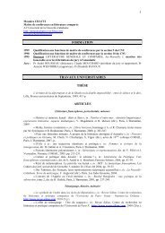
human activities chain that depend on natural resources are regularly affected by soil erosionand consequences of this phenomenon. It’s also important to note that UNESCO listed NewCaledonia Barrier Reef on the World Heritage List under the name The Lagoons of NewCaledonia: Reef Diversity and Associated Ecosystems on July 2008.The study area is located in the north of New Caledonia on west coast. This region includesthe communes of Koné, Pouembout and Voh in the North Province (Fig. 1) and 23watersheds, covering an area of 1 350 square kilometres. The study area presents a dichotomybetween a coastal plain and a mountain zone and hills covering three quarters of the region. Interms of pressures that exists in New Caledonia, this region is representative with naturalpressures due to the amount and the intensity of rainfall and the steepness of slopes and withhuman pressures to bushfires, agriculture, land-clearing by fire and mining activities. Indeed,there are several old mines (closed before 1975) in this area, not revegetated, that are stillcontributing to soil losses, as well as a new mining project on the Koniambo Mountain witchwill be the largest nickel mines in the world.Fig. 1: Location, digital elevation model and map of the study area (communes of Koné, Pouembout and Voh)III/ MATERIALS AND METHODSThe Universal Soil Loss Equation, later revised as the RUSLE (Renard et al., 1997), wasdeveloped by Wischmeier and Smith (1978). It’s a mathematical and an empirical model usedto describe soil erosion processes and based on many factors such as soil, topography,climate, land cover and human activities. The USLE predicts potential erosion and is widelyused in the world. Potential erosion, representing by soil losses, has units of weight per unitarea per year (t/ha/yr). This equation is the product of six factors:A = R x K x LX S x C x PWhere A is the average soil loss due to water erosion (t/ha/yr), R the rainfall-runoff erosivityfactor; K the soil erodibility factor, L, the slope length, S the slope steepness, C the land covermanagement factor and P the soil conservation practice factor. This model is derived frommore than 10,000 plot-years of data collected on natural runoff plots and an estimatedequivalent of 2,000 plot-years of data from rainfall simulators. Numerical values for each ofthe six factors of the equation were derived from analyses of the assembled research data andfrom National Weather Service precipitation records in USA. USLE only predicts the amountof soil loss that results from sheet or rill erosion on a single slope and does not account foradditional soil losses that might occur from gully, wind or tillage erosion. Although originallydeveloped for agricultural purpose, its use has been extended to watershed with other landuses.3

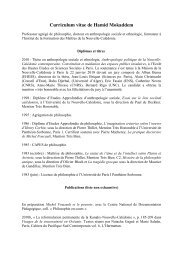
III.1/ Rainfall-runoff Erosivity: R-factorThe R factor is the climatic factor determining the erosive force of rainfall on the ground. TheR-factor is usually measured as the product (EI) of total storm energy (E) and the maximum30-min intensity (I30) for all storms over a long time (Brown and Foster, 1987). The EIparameter quantifies the effects of raindrop impact and reflects the amount and rate of runofflikely to be associated with the rain (Wischmeier and Smith, 1978). R was calculated fromthese equations:R = E × I30(1) where R is in MJ.mm ha -1 h -1 and (E) is the kinetic energy of rain in MJha -1and (I30) is the maximum 30 minute intensity in mm h −1 .The calculation of E was made from the equation derived by Brown and Foster (1987) whofound that the kinetic energy of the rain was an exponential function of the intensity of therain:E = 0 .29 × ( 1−0.72e( − 0. 05×I ))(2) where I is the rainfall intensity in mm h −1It is then possible to calculate R for a year:k1R = ∑ ( E × I ) (3) where R is in MJ.mm ha -1 h -1 yr -1 , N is number of years, K is30N i = 1number of rainy events, E is total storm kinetic energy in MJ.mm ha -1 h -1 , and I 30 is themaximum 30 minutes intensity of rain in mm h -1 .About the climate of the study area, New Caledonia lieing astride the Tropic of Capricorn,between 19° and 23° south latitude, has a tropical climate. Rainfall is highly seasonal, broughtby trade winds that usually come from the east and varies a lot according to elevation.Rainfall averages about 2 000 millimeters at low elevations on eastern “Grande Terre”, and 2000-4 000 millimeters at high elevations on the Grande Terre. The western side of the GrandeTerre lies in the rain shadow of the central mountains, and rainfall averages 1 200 millimetersper year. In the study area, rainfall varies from 500 mm/year near the sea to almost 2 000mm/year in the “Central Range”.For the computing of R factor, we use the data of 8 weather stations from Meteo France(National Meteorological Service) spread across the study area (Table 1, Fig. 2). However,these data are not insufficient for making a precise interpolation in the spatial distribution ofthe R factor. In this case, the option taken was to seek a relationship between the R factor andaltitude of stations that would extrapolate to the area. Indeed, it is not unusual that there is agradient of precipitation in relation to altitude. Thus, from a straight linear correlation (R =3.5205 x Z + 3661), 12 others “ghost stations” were computed to obtain a more preciseinterpolation. From the results of this calculation, a rainfall factor layer was then generated inthe GIS (ArcGIS) (Fig. 3) over the whole study area by using a spline interpolation on a 10meters resolution Digital Elevation Model (DEM).Table 1: Results of the R factor for the eight weather stations from Meteo FranceWeather Station R Factor (MJ.mm ha -1 h -1 yr -1 )X1 3180.54X2 3940.57X3 2142.60X4 1168.14X5 5384.04X6 2724.59X7 1886.16X8 2989.484

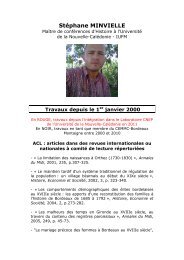
Fig.2: Localisation of the weather stationsFig.3: Spatial distribution of R factorThe R values range from 1743 to 4747 MJ.mm ha -1 h -1 yr -1 . We can observe a variation of theR factor with a spatial distribution depending on the topography. Near the coasts, the R valuesare lowest (< 2500 MJ.mm ha -1 h -1 yr -1 ), while the highest mountain ranges have high values (>4500 MJ.mm ha -1 h -1 yr -1 ).III.2/ Soil erodibility: K-factorThe soil erodibility factor (K) represents the susceptibility of a soil type to erosion. The K-factor reflects the ease with which the soil is detached by splash during rainfall and/or bysurface flow, and therefore shows the change in the soil per unit of applied external force ofenergy. This factor is related to the integrated effect of rainfall, runoff, and infiltration andaccounts for the influence of soil properties on soil loss during storm events on sloping areas.This factor is determined using inherent soil properties (Parysow et al., 2003). A simplermethod to predict K was presented by Wischmeier et al. (1971) which includes the particlesize of the soil, organic matter content, soil structure and profile permeability. The soilerodibility factor K can be approximated from a monograph if this information is known. TheUSLE monograph estimates erodibility as:1.14 −6K = 2.1×M × 10 (12 − MO)+ 0.0325×( b − 2) + 0.025×( c − 3) where M = (% silt + %very fine sand) (100- %clay), MO is the percent organic matter content, b is soil structurecode, and c is the soil permeability rating.For computing the K factor, two soil maps, one at 1/200 000 scale (Podwojewski et Beaudou,1987) available on all New Caledonia territory and the other at 1/50 000 scale available onlyon the study area (Denis et Mercky, 1982) were used. There are 22 different soils on the area(Fig. 4), but not all soils have information about structure analysis. Thus, clusters wereoperated with similar soil classes. At the end, the study area was divided into 5 major soilclasses (Table 2).Table 2: K-factors for the study areaSoil Usda class K factorAltered ferritic and ferrallitic soils Sandy loam 0.013Tropical eutrophic brown soils, hypermagnesic, on0.022Clayultrabasic rocksDesaturated fersiallitic soils Loam 0.03Little developed soils of alluvial contribution, modal with0.013Sandy loamvariable textureTropical eutrophic brown soils, little developed and modal0.022Clayon basalts5

The percentages of clay, silt, sand and organic matter were determinate for each major soiltype, and using the USDA texture triangle (Brown, 2003), the texture of each major soil typewas defined. To obtain the K factor for soil we use the chart correlating the textures and thestandard K-factor (Stone and Hillborn, 2002).Fig. 4: Soil map at 1/200 000 scaleFig. 5: Spatial distribution of K factorWith these results, the spatial distribution of the K factor was computed under a GIS at 10meters resolution (Fig. 5). We can see that most of the study area has a K factor between0.013 and 0.03 t.ha.h/ha.MJ.mm. On the areas of utramafic rocks (mining massifs), the Kfactor is relatively low. These, consisting of a hard iron crust, have a sensitivity to erosionlow. Conversely, the Central Range has a sensitivity to erosion with a high K value. This isexplained by the high percentage of sand in the fersiallitic soil who compose it, making themfragile. The coastal plain as a whole presents a medium to high sensitivity to erosionespecially in the river system in the presence of alluvial material with a high K value.III.3/ Slope length and steepness: LS-factorIn the USLE model, the effect of topography on erosion is accounted for by the slope length(L) and the slope steepness (S). The L factor is defined as the distance from the source ofrunoff to the point where either deposition begins or runoff enters a well defined channel thatmay be part of a drainage network. S factor reflects the influence of slope steepness onerosion (Wischmeier and Smith, 1978). The longer the slope length the greater the amount ofcumulative runoff. Also the steeper the slope of the land the higher the velocities of therunoff which contribute to erosion. But soil loss increases more rapidly with slope steepnessthan it does with slope length (McCool et al., 1987). The common equation used forcalculating LS factor provide by the USDA Agricultural Handbook (Wischmeier and Smith1978):m⎛ λ ⎞2LS = ⎜ ⎟ × (65.41sin θ + 4.56sinθ+ 0.065) where λ is the slope length in meters, θ⎝ 22.13⎠is the slope angle in degrees, and m is a slope angle contingent variable ranging from 0.01 to0.56 (McCool et al. 1987).For computing the LS factor, after testing different methods as Mitasova et al.(1998), wechoose to use an algorithm developed by Van Remortel et al. (2001), based on the equation ofRenard et al. (1997). Using an AML (Arc Macro Language) script under ArcInfo and aDigital Elevation Model (DEM) at 10 meters resolution, λ and θ were computed directly6

under the GIS software. The LS factor ranges from 0 to 104 with an average of 6.4 (Fig. 6).Half of the values are under 5 and correspond mostly to plain zones. The high values (superiorto 20) correspond to the crests of the mountains, more sensible to erosion. But it representsonly 7% of the area.Fig.6: Spatial distribution of LS FactorIII.4/ Cover management: C-factorThe C-factor measures the effects of all interrelated cover and management variables (Renardet al., 1997). C factor is measured as the ratio of soil loss from land cropped under specificconditions to the corresponding loss from tilled land under continuous fallow conditions. Bydefinition, C equals 1 under standard fallow conditions. As surface cover is added to the soil,the C factor value approaches zero. A C factor of 0.15 means that 15% of the amount oferosion will occur compared to continuous fallow conditions (Kesley and Johnson, 2003).The C factor was derived using remote sensing techniques. Thus, the land cover layer wasimplemented from the results of the supervised classification method (produced by DTSI)based on a SPOT 3 satellite image taken in 1996 with a 20 meters resolution (Fig. 7). Thesedata seem old but the land cover has not really changed these ten last years because the humanpressure is low in this region. The plain is covered by an extensive grass and dry niaoulissavannah over low hills and flat areas. Large areas of ultramafic rocks correspond tomountainous areas with vivid red lateritic soils covered by an endemic vegetation bush andforests of unique plants species. Along the coastal zone mangroves are present. Thedetermination of factor C depends on the coverage of the soil surface by vegetation. Frombibliographic data, we assign a coefficient C between 0 and 1 for each type of vegetation onthe study area. (Table 3). The distribution of factor C is quite heterogeneous (Fig. 8). Baresoils most erodible, are mainly located on the coast and the mountains degraded by miningactivity. The areas of dense vegetation located mainly in the hills of the “Central Chain areless susceptible to erosion.Table 3: Land cover types and C-FactorVegetation typeC FactorForest 0.001Savanna 0.04Mining scrubland 0.25Swamp 0.28Brush 0.72Bare land 17

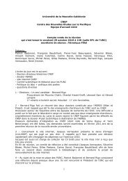
Fig.7: Thematic land cover mapFig.8: Spatial distribution of C FactorIII.5/ Support practice P-factorThe P-factor is the ratio of soil loss with specific support practice to the corresponding losswith up and downslope tillage. These practices proportionally affect erosion by modifying theflow pattern, gradient, or direction of surface runoff and by reducing the amount and rate ofrunoff. The P values are between 0 and 1. Because of a lack of information on practicesconservation tillage, we adopt P = 1 over the study area for not modify the final result.IV RESULTSAll factors layers R, LS, K, and C, computed and spatialized previously by the use of GISfunctions, are combined together to obtain a soil loss rate layer (Fig. 9). We obtain an averageof 137 t/ha/yr of potential erosion in the study area. Three-quarters of the study area (64%)have an erosion rate under 200 t/ha/yr. These areas correspond primarily to the basinfloodplains and flat areas of the “Central Chain” covered by forests. These regions are theleast sensitive to erosion. The very high estimations of soil loss (more than 1000 t/ha/yr) arelocated in 6% of the study area and correspond primarily at the top hills of the “CentralChain”. The high values of soil loss are the result of the combination of steep slopes, highprecipitation, altered soils and bare soils due to human activities, such as agriculture, landclearingby fire and mining activities located on the most sensitive areas to erosion. A firstvisual interpretation of the different factors shows that topography seems to be the dominantdriver for explaining the variation in erosion rate. The results and particularly the high valuesseem to be overestimated. The LS values will be overweighted in this analysis. In fact, theextreme slopes throughout the mountain areas do not correlate well with the USLE model,which was originally developed for mild slopes in agricultural areas. The others reasons areprobably the quality of the input data implemented in the model. The spatial scale is notadapted as the soil map for example or the typology of the land use map is not precise: it'snecessary to have more detailed land use data in which agricultural land use could beensubdivided into specific crops. The estimation of soil loss is in the same order of magnitudeas other studies: 200 to 400 t/ha/yr in Tahiti (Servant, 1974) or 200 to 500 t/ha/yr in theBurundi (Rishirumuhirwa, 1997). It’s also important to note that USLE model gives the longtermaverage soil loss resulting from sheet erosion processes. However, soil loss from othertypes of erosion, gully erosion from lavakas for example, need to be estimated.8

Fig. 9: Potential soil loss erosion in the study area. The high estimations of soil loss correspond primarily at thetop hills of the “Central Chain”. They are the result of the combination of steep slopes, high precipitation, alteredsoils and bare soils due to human activities, such as mining activities.V/ CONCLUSION AND DISCUTIONSoil erosion is a serious problem in New-Caledonia mainly due to the cyclonic tropicalweather, bush fires and human activities such as openpit mining. Runoff on stripped soilscauses degradations for anthropic laying out on high ultramafic terranes and pollution(mobilized soil particles) which modifies the coastal region and degrades the coral reefs byhypersedimentation processes. All the human activities chain that depend on natural resourcesregularly suffer the effects or the consequences of these phenomena. The situation, not for thesame reasons and not in the same proportions, is similar in others high islands of the SouthPacific such as Efate island in Vanuatu (Dumas and Fossey, 2009). These countries need toidentify and rank erosion risk and define sensitivity maps, particularly for decisionmakers. Inthis case, the USLE model can be useful for processing the potential soil erosion mapping at aregional scale, implemented with some data not too complex and compatible with theirintegration into a Geographical Information System (GIS), generally available in the Pacificcountries as a digital elevation model, a soil map, precipitation data or satellite images. Theuse of GIS becomes an important and powerful tool for the implementation of this model. TheUSLE equation used lead a better understanding of spatial distribution of the erosion hazard.Moreover, a comparison with a multi-criteria method (expert approach) demonstrates thatresults obtained in term of spatial variation are similar (Dumas et al., 2009). But the values ofsoil loss from USLE should be considered as an order of magnitude and not as absolutevalues. In fact, USLE model is useful to identify risks areas and catchments that are moresensitive to erosion. This type of mapping should be relevant to classify the reef zone mostaffected by hypersedimentation hazard. Within the framework of Integrated Coastal ZoneManagement, the areas most affected by erosion will be classified as priority managementareas so as to limit their impacts on the marine environment.ACKNOWLEDGMENTSThe authors would like to acknowledge the support of CRISP program (Coral ReefsInitiatives for the Pacific) for funding this research project.9

REFERENCESAdinarayana J, Rao KG, Krishna NR, Venkatachalam P, Suri JK., (1999). A rule-based soil erosion model for ahilly catchment. Catena 37: 309–318.Arnold J.G., Williams J.R., (1995). SWRRB - A Watershed Scale Model for Soil and Water ResourcesManagement. Computer Models of Watershed Hydrology. Highlands Ranch, CO, V. P. Singh, WaterResources Publications, pp. 847-908.Brown L.C., Foster G.R., 1987, Storm erosivity using idealized intensity distributions. Trans. ASAE 30:379-386.Brown R.B., (2003). Soil Texture. Soil and Water Science Department, Florida Cooperative Extension Service,Institute of Food and Agricultural Sciences, University of Florida, Fact Sheet SL-29, 8p.Bathurst J.C., O’Connell P.E. (1992). Future of distributed modeling – the Système Hydrologique Européen,Hydrol. Process. 6, pp. 262–277.Denis B., Mercky P., (1982). Carte pédologique de la region de Pouembout au 1:50 000. ORSTOM, Nouméa.Dumas P., (2004). Caractérisation des littoraux insulaires : approche géographique par télédétection et SIG pourune gestion intégrée, Application en Nouvelle-Calédonie. Thèse de doctorat, Orléans, 402 p.Dumas P., Printemps J.,Mangeas M., Luneau G., (2009). Developing Erosion Models for Integrated CoastalZone Management. A Case Study of New-Caledonia West Coast. Marine Polution Buletin,17p. (accepted).Dumas P., Fossey M. (2009). Mapping Potential Soil Erosion in the Pacific Islands – A case study of EfateIsland (Vanuatu). 11Th Pacific Science Inter-Congress, « Pacific Countries and their ocean, facing localand global changes » 2-6 march 2009, 5 p. (accepted).Eyles G.O. (1987). Soil Erosion in the South Pacific, Environmental Studies Report N°37, Institute of NaturalResources, University of the South Pacific.Kelsey K., and Johnson T. (2003). Determining Cover Management Values (C factors) for Surface Cover BestManagement Practices (BMPs). In Proceedings of the International Erosion Control Association’s 34thConference. CD Rom.McCool D., Brownl L., Foster G., Mutchler C., Meyerl L,. (1987). Revised slope steepness factor for the USLE.Transaction of the American Society of Agricultural Engineers 30, pp. 1387-1396.Mitasova, H., Mitas, L., Brown, W., and Johnston, D.,(1998). Multidimentional soil erosion/depositionmodelling and visualization using GIS. Final report for USA CERL. University of ILLINOIS, Urbana-Champaigne, IL.Nearing MA, Foster GR, Lane LJ, Finkner SC., (1989). A process-based soil erosion model for USDA-WaterErosion Prediction Project Technology. Transactions of the ASAE 32: 1587–1593.Neistch S. L., Arnold J.G., Kiniry J.R., Williams J.R., King K.W. (2002). Soil and Water Assessment ToolTheoretical Documentation, Version 2000. Grassland, Soil and Water Research Laboratory, U.S.Department of Agriculture Agricultural Research Service, Temple TX.Nelson D. (1987). Land conservation in the Rewa and Ba watersheds, Fiji. FAO Report to the Fiji Ministry ofPrimary Industries.Podwojewski P.,Beaudou A.G., (1987). Carte morpho-pédologique de la Nouvelle-Calédonie au 1:200 000.ORSTOM, Nouméa.Parysow P, Wang G, Gertner GZ, Anderson AB., (2003). Spatial uncertainty analysis for mapping soilerodibility based on joint sequential simulation. Catena 53: p 65-78.Renard K.G., Foster G.R., Weesies G.A., McCool, D.K., Yoder, D.C., (1997), Predicting Soil Erosion by Water:A Guide to Conservation Planning With the Revised Universal Soil Loss Equation (RUSLE). U.S.Department of Agriculture, Agriculture Handbook No. 703, 404 pRishirumuhirwa T. (1997). Rôle du bananier dans le fonctionnement des exploitations agricoles sur les hautsplateaux de l’Afrique orientale. Thèse n°1636,EPFL, Lausanne.Servant, J., (1974). Un problème de géographie physique en Polynésie Française : l’érosion, exemple de Tahiti.Cahier ORSTOM, série Sciences Humaines, vol. XI, n°3/4, pp 203-209.Shen DY, Ma AN, Lin H, Nie XH, Mao SJ, Zhang B, Shi JJ., (2003). A new approach for simulating watererosion on hillslopes. International Journal of Remote Sensing 24: 2819–2835.Simonett D.S. (1968). Selva Landscapes, pp989-990 of the Encyclopaedia of Geomorphology, Fairbridge, R.W.,Ed. Reinhold Book Corp, New York, London.Stone R.P., Hillborn D. (2002). Universal Soil Loss Equation, Ontario, Canada. Ontario Ministry of Agricultureand Food (OMAFRA).Van Remortel, R.D., Hamilton, M.E., Hickey, R.J., (2001). Estimating the LS factor for RUSLE throughiterative slope length processing of digital elevation data within ArcInfo grid. Cartography 30 (1), p 27-35.Wischmeier, W.H., Johnson, C.B. & Cross, B.V., (1971). A soil erodibility nomograph for farmland andconstruction sites, Journal of Soil and Water Conservation, 26, p 189-93.Wischmeier W.H., Smith D.D., (1978), Predicting Rainfall Erosion Losses; A guide to conservation planning,Agriculture handbook No. 537. US department of Agriculture Science and Education Administration,Washington, DC, USA, 163 p.10