Panel Data Evidence from Irrigated Rice Production in Southern

More documents

Recommendations

Info

100 PHILIPPINE JOURNAL OF DEVELOPMENTstatistical significance of labor rises, while that of fertilizer falls. The dummyvariable for tractor use remains statistically insignificant. Results providestatistical support for the existence of a stochastic frontier. Following Schmidtand Lin (1984), we use the square root of the variance ratio as the basis fortesting the existence of a frontier in Model 2. In our case the estimated value( λ = 4.12, t = 5.27) is significantly different from zero at the 95 percentconfidence level.Model 3 is a frontier model estimated using parcel-level random effects.In Model 3 all point estimates are significantly different from zero at the 95percent confidence level, with the exception of the dummy variables foryears and tractor use. Coefficients on the year dummy variables suggest thatyields were somewhat lower in 1999 than in 1995 or 1997. As in previousmodels, yields on parcels in site 2 (Tamlang) were lower on average than onthose in site 1 (Marangas). Again, yields were much higher in the rainyseason and approximately 52 percent higher in the dry season in the presenceof irrigation. A Lagrange multiplier test provides statistical evidence thatsupports the parcel-level random effects specification. For this test, we comparepanel and nonpanel regressions in the absence of a frontier. The Lagrangemultiplier test statistic is distributed with one degree of freedom. The2test statistic is 5.38, which exceeds the χ critical value of 3.84. We thereforeconclude that, in this case, an individual effects model is preferred to amodel without individual effects at a 95 percent significance level. We notethat the coefficients on labor, fertilizer, and pesticide are positive andsignificant in Model 3 and suggest diminishing returns to use of these inputs.Yields appear to be most sensitive to fertilizer application, followed by levelsof labor and pesticides, respectively.In Model 4 we relax the assumption of time-invariant productioncoefficients in order to assess the extent to which factor productivity changedover the sample period. For each input (labor, fertilizer, and pesticide), Model4 introduces two additional regression coefficients in the form of inputdummyinteraction terms for 1995 and 1997. For each input, the nullhypothesis of no change in input elasticities can be examined via a Wald test.We test the assumption that the input-year interaction terms are jointly equalto zero, i.e., that the production coefficients are constant across time. With2411 observations and two restrictions, the critical χ value is 3.00. In thecase of labor, although the coefficient values point toward labor shedding onthe part of sample farms over the period 1995-1999, the interaction terms areneither individually nor jointly significant at standard test levels (the teststatistic W = 0.63, with a ρ-value of 0.73). Results suggest that production wasmore sensitive to fertilizer use in 1997 than in 1995, and less sensitive in1999, although the interaction terms are neither individually nor jointlysignificant at standard test levels (W = 2.43, ρ = 0.30). In the case of pesticides,the year-specific coefficients are individually and jointly significant (W =
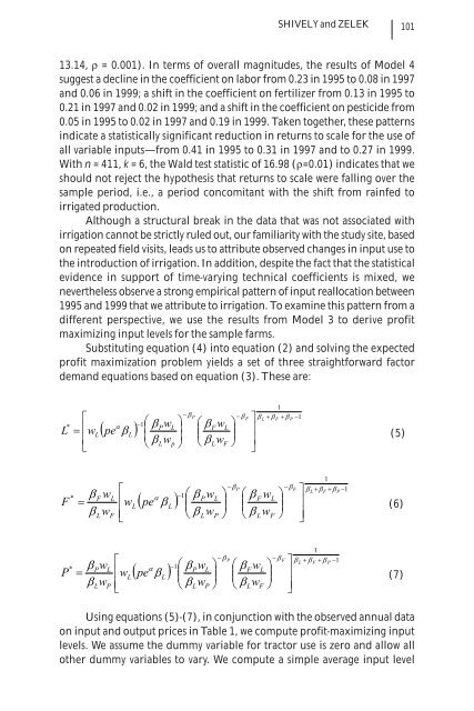
SHIVELY and ZELEK10113.14, ρ = 0.001). In terms of overall magnitudes, the results of Model 4suggest a decline in the coefficient on labor from 0.23 in 1995 to 0.08 in 1997and 0.06 in 1999; a shift in the coefficient on fertilizer from 0.13 in 1995 to0.21 in 1997 and 0.02 in 1999; and a shift in the coefficient on pesticide from0.05 in 1995 to 0.02 in 1997 and 0.19 in 1999. Taken together, these patternsindicate a statistically significant reduction in returns to scale for the use ofall variable inputs—from 0.41 in 1995 to 0.31 in 1997 and to 0.27 in 1999.With n = 411, k = 6, the Wald test statistic of 16.98 (ρ=0.01) indicates that weshould not reject the hypothesis that returns to scale were falling over thesample period, i.e., a period concomitant with the shift from rainfed toirrigated production.Although a structural break in the data that was not associated withirrigation cannot be strictly ruled out, our familiarity with the study site, basedon repeated field visits, leads us to attribute observed changes in input use tothe introduction of irrigation. In addition, despite the fact that the statisticalevidence in support of time-varying technical coefficients is mixed, wenevertheless observe a strong empirical pattern of input reallocation between1995 and 1999 that we attribute to irrigation. To examine this pattern from adifferent perspective, we use the results from Model 3 to derive profitmaximizing input levels for the sample farms.Substituting equation (4) into equation (2) and solving the expectedprofit maximization problem yields a set of three straightforward factordemand equations based on equation (3). These are:*L⎡= ⎢w⎢⎣Lα( pe )1β L + β F + β P −1−βP−βF ⎤−1⎛⎞ ⎛ ⎞⎜βPwL⎟βFwLβ ⎥L⎜⎟(5)⎝ βLwp⎠ ⎝ βLwF⎠ ⎥⎦FP**βFw=β wLβPw=β wLLPLF⎡⎢w⎢⎣⎡⎢w⎢⎣LLα( pe β )Lα( pe β )L−1−1⎛ βPw⎜⎝ βLw⎛ βPw⎜⎝ βLwLPLP⎞⎟⎠⎞⎟⎠−βP−βP⎛ βFw⎜⎝ βLw⎛ βFw⎜⎝ βLwLFLF⎞⎟⎠⎞⎟⎠−βF−βF⎤⎥⎥⎦⎤⎥⎥⎦1β L + β F + β P −11β L + β F + β P −1(6)(7)Using equations (5)-(7), in conjunction with the observed annual dataon input and output prices in Table 1, we compute profit-maximizing inputlevels. We assume the dummy variable for tractor use is zero and allow allother dummy variables to vary. We compute a simple average input level
Page 5: SHIVELY and ZELEK95season from Janu
Page 8 and 9: 98 PHILIPPINE JOURNAL OF DEVELOPMEN
Page 12 and 13: 102 PHILIPPINE JOURNAL OF DEVELOPME
Page 20: 110 PHILIPPINE JOURNAL OF DEVELOPME

Panel Data Evidence from Irrigated Rice Production in Southern

You also want an ePaper? Increase the reach of your titles

Delete template?

Save as template?