- Page 1 and 2:
Deliverable D7.5Multilevel modellin
- Page 3 and 4:
3.6 State space models.............
- Page 5 and 6:
Chapter 1 - IntroductionHeike Marte
- Page 7 and 8:
IntroductionFigure 1.2: Structure o
- Page 9 and 10:
2.1 Introduction multilevel modelli
- Page 11 and 12:
2.2 Multilevel linear regression mo
- Page 13 and 14:
2.2 Linear multilevel models Click
- Page 15 and 16:
2.2 Linear multilevel modelsResults
- Page 17 and 18:
2.2 Linear multilevel models• Cli
- Page 19 and 20:
2.2 Linear multilevel modelsThe mod
- Page 21 and 22:
2.2 Linear multilevel modelsThe siz
- Page 23 and 24:
2.2 Linear multilevel modelsResults
- Page 25:
2.2 Linear multilevel modelsResults
- Page 28 and 29:
Chapter 2intercept between location
- Page 30 and 31:
Chapter 2Results and interpretation
- Page 32 and 33:
2.3 Discrete response models2.3.1 I
- Page 34 and 35:
Chapter 2• Click on “Add Term
- Page 36 and 37:
Chapter 2Results and interpretation
- Page 38 and 39:
Chapter 2Predictor Coefficient π j
- Page 40 and 41:
2.3.3 Multinomial responsesHeike Ma
- Page 42 and 43:
Chapter 2A new response variable ha
- Page 44 and 45:
Chapter 2Results and interpretation
- Page 46 and 47:
Chapter 2ResultsAs can be seen in t
- Page 48 and 49:
Chapter 2• Select “age” from
- Page 50 and 51:
Chapter 2Results and interpretation
- Page 52 and 53:
2.3.4 CountsGeorge Yannis, Eleonora
- Page 54 and 55:
Chapter 2▪ Click on the N (ΩΧ,
- Page 56 and 57: Chapter 2These results are intuitiv
- Page 58 and 59: Chapter 2▪ In the plot what? tab,
- Page 60 and 61: Chapter 2We will now add a random s
- Page 62 and 63: Chapter 2All fixed and random effec
- Page 64 and 65: Chapter 2We can see that the level-
- Page 66 and 67: Chapter 2In this case, all fixed ef
- Page 68 and 69: Chapter 2Another issue that needs t
- Page 70 and 71: Chapter 2In the bottom line of the
- Page 72 and 73: 2.4 Longitudinal dataHeike Martense
- Page 74 and 75: Chapter 2Than open the “Names”
- Page 76 and 77: Chapter 2• Click “Calc” to ca
- Page 78 and 79: Chapter 2Results and Interpretation
- Page 80 and 81: Chapter 2Results and Interpretation
- Page 82 and 83: Chapter 2Now a variable that contai
- Page 84 and 85: Chapter 2 Click “Done”• Estim
- Page 86 and 87: Chapter 2As described in the multiv
- Page 88 and 89: Chapter 2▪ Click on resp1 or resp
- Page 90 and 91: Chapter 2Before we proceed in fitti
- Page 92 and 93: Chapter 2▪ Click on the Estimates
- Page 94 and 95: Chapter 2We will now proceed in bui
- Page 96 and 97: Chapter 2A significant regional var
- Page 98 and 99: Chapter 2▪ Click More to run the
- Page 100 and 101: Chapter 2The fixed effect of enforc
- Page 102 and 103: Chapter 3 - Time series analysis3.1
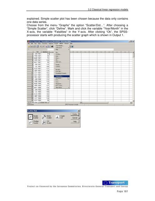
- Page 104 and 105: Chapter 3manual's objective: "even
- Page 108 and 109: Chapter 3The figure displayed below
- Page 110 and 111: Chapter 3
- Page 112 and 113: Chapter 3Then mark and click the va
- Page 114 and 115: Chapter 3The residual analysis in t
- Page 116 and 117: Chapter 3A new window “Linear Reg
- Page 118 and 119: Chapter 3The result stated above sh
- Page 120 and 121: Chapter 3The same result is obtaine
- Page 122 and 123: Chapter 3In this new opened window
- Page 124 and 125: Chapter 3To compute the last variab
- Page 126 and 127: Chapter 3
- Page 128 and 129: Chapter 3time series on “Squared
- Page 130 and 131: Chapter 33.2.2 Generalized linear m
- Page 132 and 133: Chapter 3SPSS (Version 14.0) was us
- Page 134 and 135: Chapter 33.4.2 ARIMA models for sta
- Page 136 and 137: Chapter 3• Click on Graphs..Seque
- Page 138 and 139: Chapter 3The ACF plot indicates the
- Page 140 and 141: Chapter 3The ACF plot of the filter
- Page 142 and 143: Chapter 3• Click on Statistics th
- Page 144 and 145: Chapter 3Model Description ARIMA(0,
- Page 146 and 147: Chapter 3In addition to the precedi
- Page 148 and 149: Chapter 3Note that it is very diffi
- Page 150 and 151: Chapter 3In the case the Residuals
- Page 152 and 153: Chapter 3The normal Q-Q plot compar
- Page 154 and 155: Chapter 33.4.4 ARIMA models for sea
- Page 156 and 157:
Chapter 33.4.4.2. Model identificat
- Page 158 and 159:
Chapter 3The ACF plot indicates obv
- Page 160 and 161:
Chapter 33.4.4.3. Model estimation
- Page 162 and 163:
Chapter 3• Click on Plots tab and
- Page 164 and 165:
Chapter 3Model Description ARIMA (2
- Page 166 and 167:
Chapter 33.4.4.4. Graphical results
- Page 168 and 169:
Chapter 3Kolmogorov-Smirnov TestIn
- Page 170 and 171:
Chapter 3Here are the SPSS results
- Page 172 and 173:
Chapter 3of the residuals, up to or
- Page 174 and 175:
Chapter 3HistogramQQ-plot
- Page 176 and 177:
Chapter 3As the intervention variab
- Page 178 and 179:
Chapter 3The addition of the two ex
- Page 180 and 181:
Chapter 3Histogram
- Page 182 and 183:
Chapter 3Kolmogorov-Smirnov TestIn
- Page 184 and 185:
Chapter 33.5 DRAG modelsThe DRAG mo
- Page 186 and 187:
Chapter 3a summary of results and s
- Page 188 and 189:
Chapter 3This data file consists of
- Page 190 and 191:
Chapter 3 Then click on the Finish
- Page 192 and 193:
Chapter 3Independence Q(6,6) 28.8 1
- Page 194 and 195:
Chapter 3Step 4: Graphics of model
- Page 196 and 197:
Chapter 3 Shortly examine the figur
- Page 198 and 199:
Chapter 3The STAMP graphics window
- Page 200 and 201:
Chapter 334, we better use the Door
- Page 202 and 203:
Chapter 3The auxiliary residuals ar
- Page 204 and 205:
Chapter 33.6.2.2 Stochastic level m
- Page 206 and 207:
Chapter 3convergence criteria used
- Page 208 and 209:
Chapter 36.25Log_NO_fatTrend_Log_NO
- Page 210 and 211:
Chapter 3 Go to the STAMP window ag
- Page 212 and 213:
Chapter 3 Click OK.
- Page 214 and 215:
Chapter 3The list of forecast resul
- Page 216 and 217:
Chapter 33.6.3 Local linear trend m
- Page 218 and 219:
Chapter 3Irr 0.021360 ( 1.0000) Che
- Page 220 and 221:
Chapter 3 In the Residual graphics
- Page 222 and 223:
Chapter 33.6.3.2. Stochastic linear
- Page 224 and 225:
Chapter 3Estimation sample is 1970.
- Page 226 and 227:
Chapter 37.0 Log_FI_fat Trend_Log_F
- Page 228 and 229:
Chapter 3The goodness-of-fit is cle
- Page 230 and 231:
Chapter 3The STAMP graphics window
- Page 232 and 233:
Chapter 33.6.4 Local linear trend p
- Page 234 and 235:
Chapter 3Prediction error variance
- Page 236 and 237:
Chapter 3Parameter estimation sampl
- Page 238 and 239:
Chapter 38.007.757.507.257.000.2Log
- Page 240 and 241:
Chapter 3Goodness-of-fit results fo
- Page 242 and 243:
Chapter 3interpretation of the test
- Page 244 and 245:
Chapter 3The text "Lvl 1983.2" appe
- Page 246 and 247:
Chapter 3Normality N 2.40 5.99 +Tab
- Page 248 and 249:
Chapter 32Residual Log_UKdriversKSI
- Page 250 and 251:
Chapter 32IrrRes Log_UKdriversKSI0.
- Page 252 and 253:
Chapter 33.6.6 Explanatory variable
- Page 254 and 255:
Chapter 3function has increased fro
- Page 256 and 257:
Chapter 3Figure 3.6.18: Observed lo
- Page 258 and 259:
Chapter 3 Use the menu or to save
- Page 260 and 261:
Chapter 32IrrRes Log_UKdriversKSI0.
- Page 262 and 263:
Chapter 3for this period. The actua
- Page 264 and 265:
Chapter 3the top figure and the ori
- Page 266 and 267:
Chapter 4 - ConclusionThe present d
- Page 268 and 269:
Chapter 4researchers conduct valid
- Page 270:
ReferencesLISREL for Windows. Scien