ALGORITHMS FOR SOLVING LINEAR AND POLYNOMIAL ...

ABSTRACTTitle of dissertation:ALGORITHMS FOR SOLVINGLINEAR AND POLYNOMIALSYSTEMS OF EQUATIONSOVER FINITE FIELDSWITH APPLICATIONS TOCRYPTANALYSISGregory BardDoctor of Philosophy, 2007Dissertation directed by:Professor Lawrence C. WashingtonDepartment of MathematicsThis dissertation contains algorithms for solving linear and polynomial systemsof equations over GF(2). The objective is to provide fast and exact tools for algebraiccryptanalysis and other applications. Accordingly, it is divided into two parts.The first part deals with polynomial systems. Chapter 2 contains a successfulcryptanalysis of Keeloq, the block cipher used in nearly all luxury automobiles.The attack is more than 16,000 times faster than brute force, but queries 0.6 × 2 32plaintexts. The polynomial systems of equations arrising from that cryptanalysiswere solved via SAT-solvers.Therefore, Chapter 3 introduces a new method ofsolving polynomial systems of equations by converting them into CNF-SAT problemsand using a SAT-solver. Finally, Chapter 4 contains a discussion on how SAT-solverswork internally.The second part deals with linear systems over GF(2), and other small fields(and rings). These occur in cryptanalysis when using the XL algorithm, which con-

verts polynomial systems into larger linear systems. We introduce a new complexitymodel and data structures for GF(2)-matrix operations. This is discussed in AppendixB but applies to all of Part II. Chapter 5 contains an analysis of “the Methodof Four Russians” for multiplication and a variant for matrix inversion, which islog n faster than Gaussian Elimination, and can be combined with Strassen-like algorithms.Chapter 6 contains an algorithm for accelerating matrix multiplicationover small finite fields. It is feasible but the memory cost is so high that it is mostlyof theoretical interest. Appendix A contains some discussion of GF(2)-linear algebraand how it differs from linear algebra in R and C. Appendix C discusses algorithmsfaster than Strassen’s algorithm, and contains proofs that matrix multiplication,matrix squaring, triangular matrix inversion, LUP-factorization, general matrix inversionand the taking of determinants, are equicomplex. These proofs are alreadyknown, but are here gathered into one place in the same notation.

ALGORITHMS FOR SOLVING LINEAR AND POLYNOMIALSYSTEMS OF EQUATIONS OVER FINITE FIELDS,WITH APPLICATIONS TO CRYPTANALYSISbyGregory V. BardDissertation submitted to the Faculty of the Graduate School of theUniversity of Maryland, College Park in partial fulfillmentof the requirements for the degree ofDoctor of Philosophy2007Advisory Committee:Professor Lawrence C. Washington, Chair/AdvisorProfessor William Adams,Professor Steven Tretter,Professor William Gasarch,Assistant Professor Jonathan Katz.

© Copyright byGregory V. Bard2007

PrefacePigmaei gigantum humeris impositi plusquam ipsi gigantes vident 1 .(Attributed to Bernard of Chartres, 1159)One of the many reasons the subject of Mathematics is so beautiful is thecontinuing process of building one theorem, algorithm, or conjecture upon another.This can be compared to the construction of a cathedral, where each stone gets laidupon those that came before it with great care. As each mason lays his stone hecan only be sure to put it in its proper place, and see that it rests plumb, level, andsquare, with its neighbors. From that vantage point, it is impossible to tell whatrole it will play in the final edifice, or even if it will be visible. Could George Boolehave imagined the digital computer?Another interesting point is that the cathedrals of Europe almost universallytook longer than one lifetime to build. Therefore those that laid the foundationshad absolutely no probability at all of seeing the completed work. This is true inmathematics, also. Fermat’s Last Theorem, the Kepler Conjecture, the Insolubilityof the Quintic, the Doubling of the Cube, and other well-known problems were onlysolved several centuries after they were proposed. And thus scholarly publicationis a great bridge, which provides communication of ideas (at least in one direction)across the abyss of death.On example is to contemplate the conic sections of Apollonius of Perga, (circa200 bc). Can one imagine how few of the ordinary or extraordinary persons ofWestern Europe in perhaps the seventh century ad, would know of them. Yet, 18centuries after their introduction, they would be found, by Kepler, to describe themotions of astronomical bodies. In the late twentieth century, conic sections werestudied, at least to some degree, by all high school graduates in the United Statesof America, and certainly other countries as well.Such is the nature of our business. Some papers might be read by only tenpersons in a century. All we can do is continue to work, and hope that the knowledgewe create is used for good and not for ill.An old man, going a lone highway,Came at the evening, cold and gray,To a chasm, vast and deep and wide,Through which was flowing a sullen tide.The old man crossed in the twilight dim;The sullen stream had no fears for him;But he turned when safe on the other sideAnd built a bridge to span the tide.“Old man,” said a fellow pilgrim near,“You are wasting strength with building here;Your journey will end with the ending day;You never again must pass this way;1 Dwarves, standing on the shoulders of giants, can further than giants see.ii

You have crossed the chasm, deep and wide—Why build you the bridge at the eventide?”The builder lifted his old gray head:“Good friend, in the path I have come,” he said,“There followeth after me todayA youth whose feet must pass this way.This chasm that has been naught to meTo that fair-haired youth may a pitfall be.He, too, must cross in the twilight dim;Good friend, I build this bridge for him.”by William Allen Drumgooleiii

ForewordThe ignoraunte multitude doeth, but as it was euer wonte, enuie thatknoweledge, whiche thei can not attaine, and wishe all men ignoraunt,like unto themself. . . Yea, the pointe in Geometrie, and the unitie inArithmetike, though bothe be undiuisible, doe make greater woorkes,& increase greater multitudes, then the brutishe bande of ignoraunce ishable to withstande. . .But yet one commoditie moare. . . I can not omitte. That is the filying,sharpenyng, and quickenyng of the witte, that by practice of Arithmetikedoeth insue. It teacheth menne and accustometh them, so certainlyto remember thynges paste: So circumspectly to consider thyngespresente: And so prouidently to forsee thynges that followe: that it maietruelie bee called the File of witte.(Robert Recorde, 1557, quoted from [vzGG03, Ch. 17]).iv

DedicationWith pleasure, I dedicate this dissertation to my parents. To my father, whotaught me much in mathematics, most especially calculus, years earlier than I wouldhave been permitted to see it. And to my mother, who has encouraged me in everyendeavor.v

AcknowledgmentsI am deeply indebted to my advisor, Professor Lawrence C. Washington, whohas read and re-read many versions of this document, and every other research paperI have written to date, provided me with countless hours of his time, and given mesound advice, on matters technical, professional and personal. He has had manystudents, and all I have spoken to are in agreement that he is a phenomenal advisor,and it is humbling to know that we can never possibly equal him. We can only tryto emulate him.I have been very fortunate to work with Dr. Nicolas T. Courtois, currentlySenior Lecturer at the University College of London. It suffices to say that the fieldof algebraic cryptanalysis has been revolutionized by his work.He permitted meto study with him for four months in Paris, and later even to stay at his home inEngland. Much of my work is joint work with him.My most steadfast supporter has been my best friend and paramour, PatrickStuddard. He has read every paper I have written to date, even this dissertation.He has listened to me drone on about topics like group theory or ring theory andhas tolerated my workaholism. My life and my work would be much more emptywithout him.My first autonomous teaching experience was at American University, a majorstepping stone in my life. The Department of Computer Science, Audio Technologyand Physics had faith in me and put their students in my hands. I am so very gratefulfor those opportunities. In particular I would like to thank Professor Michael Gray,vi

and Professor Angela Wu, who gave me much advice. The departmental secretary,Yana Shabaev was very kind to me on numerous occasions and I am grateful forall her help.I also received valuable teaching advice from my future father-inlaw,Emeritus Professor Albert Studdard, of the Philosophy Department at theUniversity of North Carolina at Pembroke.My admission to the Applied Mathematics and Scientific Computation (AMSC)Program at the University of Maryland was unusual. I had been working as a PhDstudent in Computer Engineering for several years when I decided to add a Mastersin AMSC as a side task. Later, I switched, and made it the focus of my PhD.Several faculty members were important in helping me make that transition, includingProfessor Virgil D. Gligor, Professor Richard Schwartz, and Professor JonathanRosenberg. But without the program chair, Professor David Levermore, and myadvisor, Professor Lawrence C. Washington, this would have been impossible. I amgrateful that many rules were bent.Several governmental agencies have contributed to my education. In reversechronological order,ˆ The National Science Foundation (NSF) VIGRE grant to the University ofMaryland provided the Mathematics Department with funds for “DissertationCompletion Fellowships.” These are exceedingly generous semester-long giftsand I had the pleasure to receive two of them. I am certain this dissertationwould look very different without that valuable support.ˆ I furthermore received travel funding and access to super-computing under thevii

NSF grant for the Sage project [sag], Grant Number 0555776.ˆ The European Union established the ECRYPT organization to foster researchamong cryptographers. The ECRYPT foundation was kind enough to supportme during my research visit in Paris. Much of the work of this dissertationwas done while working there.ˆ The Department of the Navy, Naval Sea Systems Command, Carderock Station,supported me with a fascinating internship during the summer of 2003.They furthermore allowed me to continue some cryptologic research towardmy graduate degrees while working there.ˆ The National Security Agency was my employer from May of 1998 untilSeptember of 2002. Not only did I have the chance to work alongside andlearn from some of the most dedicated and professional engineers, computerscientists and mathematicians who have ever been assembled into one organization,but also I was given five semesters of financial support, plus severalsummer sessions, which was very generous, especially considering that two ofthose semesters and one summer were during wartime. Our nation owes anenormous debt to the skill, perseverance, self-discipline, and creativity of theemployees of the National Security Agency. Several employees there were supportersof my educational hopes but security regulations and agency traditionswould forbid my mentioning them by name.Professor Virgil D. Gligor, Professor Jonathan Katz, and Professor WilliamR. Franklin (of RPI), have all been my academic advisor at one time or anotherviii

and I thank them for their guidance. Each has taught me from their own view ofcomputer security and it is interesting how many points of view there really are.Our field is enriched by this diversity of scholarly background. Likewise Dr HaroldSnider gave me important advice during my time at Oxford. My Oxford days werean enormous influence on my decision to switch into Applied Mathematics fromComputer Engineering.My alma mater, the Rensselaer Polytechnic Institute, has furnished me withmany skills. I cannot imagine a better training ground. My engineering degreewas sufficiently mathematically rigorous that I succeeded in a graduate program inApplied Mathematics, without having a Bachelor’s degree in Mathematics. In fact,only two courses, Math 403, Abstract Algebra, and Math 404 Field Theory, weremy transition. Yet I was practical enough to hired into and promoted several timesat the NSA, from a Grade 6 to a Grade 11 (out of a maximum of 15), including severalcommendations and a Director’s Star. I am particularly indebted to the facultythere, and its founder, Stephen Van Rensselaer, former governor of New York and(twice) past Grand Master of Free & Accepted Masons of the State of New York. Itwas at Rensselaer that I learned of and was initiated into Freemasonry, and the Institute’smission of educating “the sons of farmers and mechanics” with “knowledgeand thoroughness” echoes the teachings of Freemasonry. My two greatest friends,chess partners, and Brother Freemasons, Paul Bello and Abram Claycomb, wereinitiated there as well, and I learned much in discussions with them.I learned of cryptography at a very young age, perhaps eight years old or so.Dr. Haig Kafafian, also a Freemason and a family friend, took me aside after Churchix

for many years and taught me matrices, classical cryptography, and eventually,allowed me to be an intern at his software development project to make devices toaid the handicapped. There I met Igor Kalatian, who taught me the C language. Iam grateful to them both.x

Table of ContentsList of TablesList of FiguresList of Abbreviationsxvxviixix1 Summary 1I Polynomial Systems 52 An Extended Example: The Block-Cipher Keeloq 62.1 Special Acknowledgment of Joint Work . . . . . . . . . . . . . . . . . 72.2 Notational Conventions and Terminology . . . . . . . . . . . . . . . . 72.3 The Formulation of Keeloq . . . . . . . . . . . . . . . . . . . . . . . . 82.3.1 What is Algebraic Cryptanalysis? . . . . . . . . . . . . . . . . 82.3.2 The CSP Model . . . . . . . . . . . . . . . . . . . . . . . . . . 82.3.3 The Keeloq Specification . . . . . . . . . . . . . . . . . . . . . 92.3.4 Modeling the Non-linear Function . . . . . . . . . . . . . . . . 102.3.5 I/O Relations and the NLF . . . . . . . . . . . . . . . . . . . 112.3.6 Disposing of the Secret Key Shift-Register . . . . . . . . . . . 122.3.7 Describing the Plaintext Shift-Register . . . . . . . . . . . . . 122.3.8 The Polynomial System of Equations . . . . . . . . . . . . . . 132.3.9 Variable and Equation Count . . . . . . . . . . . . . . . . . . 142.3.10 Dropping the Degree to Quadratic . . . . . . . . . . . . . . . 142.3.11 Fixing or Guessing Bits in Advance . . . . . . . . . . . . . . . 162.3.12 The Failure of a Frontal Assault . . . . . . . . . . . . . . . . . 162.4 Our Attack . . . . . . . . . . . . . . . . . . . . . . . . . . . . . . . . 182.4.1 A Particular Two Function Representation . . . . . . . . . . . 182.4.2 Acquiring an f (8)k-oracle . . . . . . . . . . . . . . . . . . . . . 182.4.3 The Consequences of Fixed Points . . . . . . . . . . . . . . . . 192.4.4 How to Find Fixed Points . . . . . . . . . . . . . . . . . . . . 202.4.5 How far must we search? . . . . . . . . . . . . . . . . . . . . . 222.4.6 Fraction of Plainspace Required . . . . . . . . . . . . . . . . . 232.4.7 Comparison to Brute Force . . . . . . . . . . . . . . . . . . . 252.4.8 Some Lemmas . . . . . . . . . . . . . . . . . . . . . . . . . . . 262.4.9 Cycle Lengths in a Random Permutation . . . . . . . . . . . . 292.5 Summary . . . . . . . . . . . . . . . . . . . . . . . . . . . . . . . . . 322.6 A Note about Keeloq’s Utilization . . . . . . . . . . . . . . . . . . . . 34xi

3 Converting MQ to CNF-SAT 353.1 Summary . . . . . . . . . . . . . . . . . . . . . . . . . . . . . . . . . 353.2 Introduction . . . . . . . . . . . . . . . . . . . . . . . . . . . . . . . . 363.2.1 Application to Cryptanalysis . . . . . . . . . . . . . . . . . . . 373.3 Notation and Definitions . . . . . . . . . . . . . . . . . . . . . . . . . 393.4 Converting MQ to SAT . . . . . . . . . . . . . . . . . . . . . . . . . . 403.4.1 The Conversion . . . . . . . . . . . . . . . . . . . . . . . . . . 403.4.1.1 Minor Technicality . . . . . . . . . . . . . . . . . . . 403.4.2 Measures of Efficiency . . . . . . . . . . . . . . . . . . . . . . 433.4.3 Preprocessing . . . . . . . . . . . . . . . . . . . . . . . . . . . 453.4.4 Fixing Variables in Advance . . . . . . . . . . . . . . . . . . . 463.4.4.1 Parallelization . . . . . . . . . . . . . . . . . . . . . 483.4.5 SAT-Solver Used . . . . . . . . . . . . . . . . . . . . . . . . . 483.4.5.1 Note About Randomness . . . . . . . . . . . . . . . 483.5 Experimental Results . . . . . . . . . . . . . . . . . . . . . . . . . . . 493.5.1 The Source of the Equations . . . . . . . . . . . . . . . . . . . 503.5.2 The Log-Normal Distribution of Running Times . . . . . . . . 503.5.3 The Optimal Cutting Number . . . . . . . . . . . . . . . . . . 523.5.4 Comparison with MAGMA, Singular . . . . . . . . . . . . . . 553.6 Previous Work . . . . . . . . . . . . . . . . . . . . . . . . . . . . . . 553.7 Conclusions . . . . . . . . . . . . . . . . . . . . . . . . . . . . . . . . 573.8 Cubic Systems . . . . . . . . . . . . . . . . . . . . . . . . . . . . . . . 573.9 NP-Completeness of MQ . . . . . . . . . . . . . . . . . . . . . . . . . 604 How do SAT-Solvers Operate? 624.1 The Problem Itself . . . . . . . . . . . . . . . . . . . . . . . . . . . . 624.1.1 Conjunctive Normal Form . . . . . . . . . . . . . . . . . . . . 634.2 Chaff and its Descendants . . . . . . . . . . . . . . . . . . . . . . . . 644.2.1 Variable Management . . . . . . . . . . . . . . . . . . . . . . . 644.2.2 The Method of Watched Literals . . . . . . . . . . . . . . . . 664.2.3 How to Actually Make This Happen . . . . . . . . . . . . . . 664.2.4 Back-Tracking . . . . . . . . . . . . . . . . . . . . . . . . . . . 684.3 Enhancements to Chaff . . . . . . . . . . . . . . . . . . . . . . . . . . 704.3.1 Learning . . . . . . . . . . . . . . . . . . . . . . . . . . . . . . 704.3.2 The Alarm Clock . . . . . . . . . . . . . . . . . . . . . . . . . 714.3.3 The Third Finger . . . . . . . . . . . . . . . . . . . . . . . . . 714.4 Walk-SAT . . . . . . . . . . . . . . . . . . . . . . . . . . . . . . . . . 724.5 Economic Motivations . . . . . . . . . . . . . . . . . . . . . . . . . . 72II Linear Systems 745 The Method of Four Russians 755.1 Origins and Previous Work . . . . . . . . . . . . . . . . . . . . . . . . 765.1.1 Strassen’s Algorithm . . . . . . . . . . . . . . . . . . . . . . . 77xii

5.2 Rapid Subspace Enumeration . . . . . . . . . . . . . . . . . . . . . . 785.3 The Four Russians Matrix Multiplication Algorithm . . . . . . . . . . 805.3.1 Role of the Gray Code . . . . . . . . . . . . . . . . . . . . . . 815.3.2 Transposing the Matrix Product . . . . . . . . . . . . . . . . . 825.3.3 Improvements . . . . . . . . . . . . . . . . . . . . . . . . . . . 825.3.4 A Quick Computation . . . . . . . . . . . . . . . . . . . . . . 825.3.5 M4RM Experiments Performed by SAGE Staff . . . . . . . . . 835.4 The Four Russians Matrix Inversion Algorithm . . . . . . . . . . . . . 845.4.1 Stage 1: . . . . . . . . . . . . . . . . . . . . . . . . . . . . . . 865.4.2 Stage 2: . . . . . . . . . . . . . . . . . . . . . . . . . . . . . . 865.4.3 Stage 3: . . . . . . . . . . . . . . . . . . . . . . . . . . . . . . 865.4.4 A Curious Note on Stage 1 of M4RI . . . . . . . . . . . . . . . 875.4.5 Triangulation or Inversion? . . . . . . . . . . . . . . . . . . . . 905.5 Experimental and Numerical Results . . . . . . . . . . . . . . . . . . 915.6 Exact Analysis of Complexity . . . . . . . . . . . . . . . . . . . . . . 965.6.1 An Alternative Computation . . . . . . . . . . . . . . . . . . . 975.6.2 Full Elimination, not Triangular . . . . . . . . . . . . . . . . . 985.6.3 The Rank of 3k Rows, or Why k + ɛ is not Enough . . . . . . 995.6.4 Using Bulk Logical Operations . . . . . . . . . . . . . . . . . . 1015.6.5 M4RI Experiments Performed by SAGE Staff . . . . . . . . . 1025.6.5.1 Determination of k . . . . . . . . . . . . . . . . . . . 1025.6.5.2 Comparison to Magma . . . . . . . . . . . . . . . . . 1025.6.5.3 The Transpose Experiment . . . . . . . . . . . . . . 1035.7 Pairing With Strassen’s Algorithm for Matrix Multiplication . . . . . 1035.8 The Unsuitability of Strassen’s Algorithm for Inversion . . . . . . . . 1055.8.1 Bunch and Hopcroft’s Solution . . . . . . . . . . . . . . . . . 1075.8.2 Ibara, Moran, and Hui’s Solution . . . . . . . . . . . . . . . . 1086 An Impractical Method of Accelerating Matrix Operations in Rings of FiniteSize 1136.1 Introduction . . . . . . . . . . . . . . . . . . . . . . . . . . . . . . . . 1136.1.1 Feasibility . . . . . . . . . . . . . . . . . . . . . . . . . . . . . 1146.2 The Algorithm over a Finite Ring . . . . . . . . . . . . . . . . . . . . 1156.2.1 Summary . . . . . . . . . . . . . . . . . . . . . . . . . . . . . 1166.2.2 Complexity . . . . . . . . . . . . . . . . . . . . . . . . . . . . 1166.2.3 Taking Advantage of z ≠ 1 . . . . . . . . . . . . . . . . . . . . 1186.2.4 The Transpose of Matrix Multiplication . . . . . . . . . . . . 1186.3 Choosing Values of b . . . . . . . . . . . . . . . . . . . . . . . . . . . 1196.3.1 The “Conservative” Algorithm . . . . . . . . . . . . . . . . . . 1196.3.2 The “Liberal” Algorithm . . . . . . . . . . . . . . . . . . . . . 1206.3.3 Comparison . . . . . . . . . . . . . . . . . . . . . . . . . . . . 1226.4 Over Finite Fields . . . . . . . . . . . . . . . . . . . . . . . . . . . . . 1226.4.1 Complexity Penalty . . . . . . . . . . . . . . . . . . . . . . . . 1236.4.2 Memory Requirements . . . . . . . . . . . . . . . . . . . . . . 1236.4.3 Time Requirements . . . . . . . . . . . . . . . . . . . . . . . . 124xiii

6.4.4 The Conservative Algorithm . . . . . . . . . . . . . . . . . . . 1246.4.5 The Liberal Algorithm . . . . . . . . . . . . . . . . . . . . . . 1256.5 Very Small Finite Fields . . . . . . . . . . . . . . . . . . . . . . . . . 1256.6 Previous Work . . . . . . . . . . . . . . . . . . . . . . . . . . . . . . 1286.7 Notes . . . . . . . . . . . . . . . . . . . . . . . . . . . . . . . . . . . . 1286.7.1 Ring Additions . . . . . . . . . . . . . . . . . . . . . . . . . . 1286.7.2 On the Ceiling Symbol . . . . . . . . . . . . . . . . . . . . . . 129A Some Basic Facts about Linear Algebra over GF(2) 131A.1 Sources . . . . . . . . . . . . . . . . . . . . . . . . . . . . . . . . . . . 131A.2 Boolean Matrices vs GF(2) Matrices . . . . . . . . . . . . . . . . . . 131A.3 Why is GF(2) Different? . . . . . . . . . . . . . . . . . . . . . . . . . 131A.3.1 There are Self-Orthogonal Vectors . . . . . . . . . . . . . . . . 132A.3.2 Something that Fails . . . . . . . . . . . . . . . . . . . . . . . 132A.3.3 The Probability a Random Square Matrix is Singular or Invertible. . . . . . . . . . . . . . . . . . . . . . . . . . . . . . 133B A Model for the Complexity of GF(2)-Operations 135B.1 The Cost Model . . . . . . . . . . . . . . . . . . . . . . . . . . . . . . 135B.1.1 Is the Model Trivial? . . . . . . . . . . . . . . . . . . . . . . . 136B.1.2 Counting Field Operations . . . . . . . . . . . . . . . . . . . . 136B.1.3 Success and Failure . . . . . . . . . . . . . . . . . . . . . . . . 137B.2 Notational Conventions . . . . . . . . . . . . . . . . . . . . . . . . . . 137B.3 To Invert or to Solve? . . . . . . . . . . . . . . . . . . . . . . . . . . 138B.4 Data Structure Choices . . . . . . . . . . . . . . . . . . . . . . . . . . 138B.4.1 Dense Form: An Array with Swaps . . . . . . . . . . . . . . . 139B.4.2 Permutation Matrices . . . . . . . . . . . . . . . . . . . . . . . 139B.5 Analysis of Classical Techniques with our Model . . . . . . . . . . . . 140B.5.1 Naïve Matrix Multiplication . . . . . . . . . . . . . . . . . . . 140B.5.2 Matrix Addition . . . . . . . . . . . . . . . . . . . . . . . . . 140B.5.3 Dense Gaussian Elimination . . . . . . . . . . . . . . . . . . . 140B.5.4 Strassen’s Algorithm for Matrix Multiplication . . . . . . . . . 142C On the Exponent of Certain Matrix Operations 145C.1 Very Low Exponents . . . . . . . . . . . . . . . . . . . . . . . . . . . 145C.2 The Equicomplexity Theorems . . . . . . . . . . . . . . . . . . . . . . 146C.2.1 Starting Point . . . . . . . . . . . . . . . . . . . . . . . . . . . 147C.2.2 Proofs . . . . . . . . . . . . . . . . . . . . . . . . . . . . . . . 147C.2.3 A Common Misunderstanding . . . . . . . . . . . . . . . . . . 153Bibliography 154xiv

List of Tables2.1 Fixed points of random permutations and their 8th powers . . . . . . 223.1 CNF Expression Difficulty Measures for Quadratic Systems, by CuttingNumber . . . . . . . . . . . . . . . . . . . . . . . . . . . . . . . . 453.2 Running Time Statistics in Seconds . . . . . . . . . . . . . . . . . . . 543.3 Speeds of Comparison Trials between Magma, Singular and ANFtoCNF-MiniSAT . . . . . . . . . . . . . . . . . . . . . . . . . . . . . . . . . . 563.4 CNF Expression Difficulty Measures for Cubic Systems, by CuttingNumber . . . . . . . . . . . . . . . . . . . . . . . . . . . . . . . . . . 595.1 M4RM Running Times versus Magma . . . . . . . . . . . . . . . . . 845.2 Confirmation that k = 0.75 log 2 n is not a good idea. . . . . . . . . . 845.3 Probabilities of a Fair-Coin Generated n × n matrix over GF(2), havinggiven Nullity . . . . . . . . . . . . . . . . . . . . . . . . . . . . . 915.4 Experiment 1— Optimal Choices of k, and running time in seconds. . 945.5 Running times, in msec, Optimization Level 0 . . . . . . . . . . . . . 945.6 Percentage Error for Offset of K, From Experiment 1 . . . . . . . . . 955.7 Results of Experiment 3—Running Times, Fixed k=8 . . . . . . . . . 1105.8 Experiment 2—Running times in seconds under different Optimizations,k=8 . . . . . . . . . . . . . . . . . . . . . . . . . . . . . . . . . 1105.9 Trials between M4RI and Gaussian Elimination (msec) . . . . . . . . 1115.10 The Ineffectiveness of the Transpose Trick . . . . . . . . . . . . . . . 1115.11 Optimization Level 3, Flexible k . . . . . . . . . . . . . . . . . . . . . 1126.1 The Speed-Up and Extra Memory Usage given by the four choices . . 1266.2 Memory Required (in bits) and Speed-Up Factor (w/Strassen) forVarious Rings . . . . . . . . . . . . . . . . . . . . . . . . . . . . . . . 127xv

B.1 Algorithms and Performance, for m × n matrices . . . . . . . . . . . 144xvi

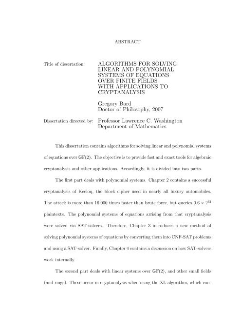
List of Figures2.1 The Keeloq Circuit Diagram . . . . . . . . . . . . . . . . . . . . . . . 93.1 The Distribution of Running Times, Experiment 1 . . . . . . . . . . . 513.2 The Distribution of the Logarithm of Running Times, Experiment 1 . 525.1 A Plot of M4RI’s System Solving in Sage vs Magma . . . . . . . . . 104C.1 The Relationship of the Equicomplexity Proofs . . . . . . . . . . . . . 147xvii

List of Algorithms1 Method of Four Russians, for Matrix Multiplication . . . . . . . . . . 802 Method of Four Russians, for Inversion . . . . . . . . . . . . . . . . . 853 The Finite-Ring Algorithm . . . . . . . . . . . . . . . . . . . . . . . . 1164 Fast M b (R) multiplications for R a finite field but not GF(2) . . . . . 1235 Gram-Schmidt, over a field of characteristic zero. . . . . . . . . . . . 1326 To compose two row swap arrays r and s, into t . . . . . . . . . . . . 1397 To invert a row swap array r, into s . . . . . . . . . . . . . . . . . . . 1408 Naïve Matrix Multiplication . . . . . . . . . . . . . . . . . . . . . . . 1409 Dense Gaussian Elimination, for Inversion . . . . . . . . . . . . . . . 14110 Dense Gaussian Elimination, for Triangularization . . . . . . . . . . . 14211 Strassen’s Algorithm for Matrix Multiplication . . . . . . . . . . . . . 142xviii

List of Abbreviationsf(x) = o(g(x))f(x)lim x→∞ g(x)f(x) = O(g(x)) ∃c, n 0 ∀n > n 0 f(x) ≤ cg(x)f(x) = Ω(g(x)) ∃c, n 0 ∀n > n 0 f(x) ≥ cg(x)f(x) = ω(g(x))g(x)lim x→∞ f(x)f(x) = Θ(g(x))f(x) ∼ g(x)Cnf-SatDesGF(q)HfeM4rmM4riMcMqOwfQuadRrefSageSatUutff(x) = O(g(x)) while simultaneously f(x) = Ω(g(x))lim x→∞f(x)g(x) = 1The conjunctive normal form satisfiability problemThe Data Encryption StandardThe finite field of size qHidden Field Equations (a potential trap-door OWF)The Method of Four Russians for matrix multiplicationThe Method of Four Russians for matrix inversionThe Multivariate Cubic problemThe Multivariate Quadratic problemOne-way FunctionThe stream cipher defined in [BGP05]Reduced Row Echelon FormSoftware for Algebra and Geometry ExperimentationThe satisfiability problemUnit Upper Triangular Formxix

Chapter 1SummaryGenerally speaking, it has been the author’s objective to generate efficient andreliable computational tools to assist algebraic cryptanalysts. In practice, this is aquestion of developing tools for systems of equations, which may be dense or sparse,linear or polynomial, over GF(2) or one of its extension fields.In addition, theauthor has explored the cryptanalysis of block ciphers and stream ciphers, targetingthe block ciphers Keeloq and the Data Encryption Standard (Des), and the streamcipher Quad. Only Keeloq is presented here, because the work on the last two arestill underway. The work on Des has seen preliminary publication in [CB06].The dissertation is divided into two parts. The first deals with polynomialsystems and actual cryptanalysis. The second deals with linear systems. Linearsystems are important to cryptanalysis because of the XL algorithm [CSPK00], astandard method of solving overdefined polynomial systems of equations over finitefields by converting them into linear systems.Chapter 2 is the most practical, and contains a detailed study of the blockcipher Keeloq and presents a successful algebraic cryptanalysis attack. The cipherKeeloq is used in the key-less entry systems of nearly all luxury automobiles. Ourattack is 2 14.77 times faster than brute force, but requires 0.6 × 2 32 plaintexts.Chapter 3 has the largest potential future impact, and deals not with linear1

systems but with polynomial systems. Also, it deals not only with dense systems(as Part II does), but with sparse systems also. Since it is known that solving aquadratic system of equations is NP-hard, and solving the Cnf-Sat problem is NPhard,and since all NP-Complete problems are polynomially reducible to each other,it makes sense to look for a method to use one in solving the other. This chaptershows how to convert quadratic systems of equations into Cnf-Sat problems, andthat using off-the-shelf Sat-solvers is an efficient method of solving this difficultproblem.Chapter 4 describes in general terms how Sat-solvers work. This tool is oftenviewed as a black box, which is unfortunate. There is no novel work in this chapter,except the author does not know of any other exposition on how these tools operate,either for experts or a general audience.The second part begins with Chapter 5, and contains the Method of FourRussians, which is an algorithm published in the 1970s, but mostly forgotten since,for calculating a step of the transitive closure of a digraph, and thus also squaringboolean matrices. Later it was adapted to matrix multiplication. This chapterprovides an analysis of that algorithm, but also shows a related algorithm for matrixinversion that was anecdotally known among some French cryptanalysts. However,the algorithm was not frequently used because it was unclear how to eliminate theprobability of abortion, how to handle memory management, and how to optimizethe algorithm. The changes have made negligible the probability of abortion, andhave implemented the algorithm so that it outperforms Magma [mag] in some cases.The software tool Sage [sag], which is an open source competitor to Magma, has2

adopted the author’s software library (built on the Method of Four Russians) for itsdense GF(2)-matrix operations, and this code is now deployed.Chapter 6 has an algorithm of theoretical interest, but which may find somepractical application as well. This algorithm is for finite-ring matrix multiplication,with special attention and advantage to the finite-field case. The algorithm takesany “baseline” matrix multiplication algorithm which works over general rings, ora class of rings that includes finite rings, and produces a faster version tailored toa specific finite ring. However, the memory required is enormous. Nonetheless, it isfeasible for certain examples. The algorithm is based on the work of Atkinson andSantoro [AS88], but introduces many more details, optimizations, techniques, anddetailed analysis.This chapter also modifies Atkinson and Santoro’s complexitycalculations.Three appendices are found, which round out Part II. Appendix A containssome discussion of GF(2)-linear algebra and how it differs from linear algebra in Rand C. These facts are well-known.We introduce a new complexity model and data structures for GF(2)-matrixoperations. This is discussed in Appendix B but applies to all of Part II.Appendix C discusses algorithms faster than Strassen’s algorithm, and containsproofs that matrix multiplication, matrix squaring, triangular matrix inversion,LUP-factorization, general matrix inversion and the taking of determinants,are equicomplex. These proofs are already known, but are here gathered into oneplace in the same notation.Finally, two software libraries were created during the dissertation work. The3

first was a very carefully coded GF(2)-matrix operations and linear algebra library,that included the Method of Four Russians. This library was adopted by Sage,and is written in traditional ANSI C. The second relates to Sat-solvers, and isa Java library for converting polynomials into Cnf-Sat problems. I have decidedthat these two libraries are to be made publicly available, as soon as the formalitiesof submitting the dissertation are completed. (the first is already available underthe GPL—Gnu Public License).4

Part IPolynomial Systems5

Chapter 2An Extended Example: The Block-Cipher KeeloqThe purpose of this chapter is to supply a new, feasible, and economicallyrelevant example of algebraic cryptanalysis. The block cipher “Keeloq” 1 is used inthe keyless-entry system of most luxury automobiles. It has a secret key consistingof 64 bits, takes a plaintext of 32 bits, and outputs a ciphertext of 32 bits. Thecipher consists of 528 rounds. Our attack is faster than brute force by a factor ofaround 2 14.77 as shown in Section 2.4.7 on page 26. A summary will be given inSection 2.5 on page 32.This attack requires around 0.6×2 32 plaintexts, or 60% of the entire dictionary,as calculated in Section 2.4.5 on page 22. This chapter is written in the “chosenplaintext attack” model, in that we assume that we can request the encryption ofany plaintext and receive the corresponding ciphertext as encrypted under the secretkey that we are to trying guess. This will be mathematically represented by oracleaccess to E k ( ⃗ P ) = ⃗ C.However, it is easy to see that random plaintexts wouldpermit the attack to proceed identically.1 This is to be pronounced “key lock.”6

2.1 Special Acknowledgment of Joint WorkThe work described in this chapter was performed during a two-week visitwith the Information Security Department of the University College of London’sIpswich campus. During that time the author worked withNicolas T. Courtois.The content of this chapter is joint work. Nonetheless, the author has rewrittenthis text in his own words and notation, distinct from the joint paper [CB07]. Someproofs are found here which are not found in the paper.2.2 Notational Conventions and TerminologyEvaluating the function f eight times will be denoted f (8) .For any l-bit sequence, the least significant bit is numbered 0 and the mostsignificant bit is numbered l − 1.If h(x) = x for some function h, then x is a fixed point of h. If h(h(x)) = xbut h(x) ≠ x then x is a “point of order 2” of h. In like manner, if h (i) (x) = x buth (j) (x) ≠ x for all j < i, then x is a “point of order i” of h. Obviously if x is a pointof order i of h, thenh (j) (x) = x if and only if i|j7

2.3 The Formulation of Keeloq2.3.1 What is Algebraic Cryptanalysis?Given a particular cipher, algebraic cryptanalysis consists of two steps. First,one must convert the cipher and possibly some supplemental information (e.g. fileformats) into a system of polynomial equations, usually over GF(2), but sometimesover other rings. Second, one must solve the system of equations and obtain fromthe solution the secret key of the cipher.This chapter deals with the first steponly. The systems of equations were solved with Singular [sin], Magma [mag], andwith the techniques of Chapter 3, as well as ElimLin, software by Nicolas Courtoisdescribed in [CB06].2.3.2 The CSP ModelIn any constraint satisfaction problem, there are several constraints in severalvariables, including the key. A solution must satisfy all constraints, so there arepossibly zero, one, or more than one solution.The constraints are models of acipher’s operation, representing known facts as equations.Most commonly, thisincludes µ plaintext-ciphertext pairs, P 1 , . . . , P µ and C 1 , . . . , C µ , and the µ facts:E(P i ) = C i for all i ∈ {1, . . . , µ}. Almost always there are additional constraintsand variables besides these.If no false assumptions are made, because these messages were indeed sent,we know there must be a key that was used, and so at least one key satisfies allthe constraints. And so it is either the case that there are one, or more than one8

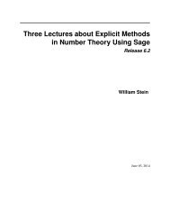
Figure 2.1: The Keeloq Circuit Diagramsolution. Generally, algebraic cryptanalysis consists of writing enough constraintsto reduce the number of possible keys to one, and few enough that the system issolvable in a reasonable amount of time. In particular, the entire process should befaster than brute force by some margin.2.3.3 The Keeloq SpecificationIn Figure 2.1 on page 9, the diagram for Keeloq is given. The top rectangleis a 32-bit shift-register. It initially is filled with the plaintext. At each round, it isshifted one bit to the right, and a new bit is introduced. The computation of thisbit is the heart of the cipher.Five particular bits of the top shift-register are and are interpreted as a 5-bit9

integer, between 0 and 31.Then a non-linear function is applied, which will bedescribed shortly (denoted NLF).Meanwhile the key is placed initially in a 64-bit shift-register, which is alsoshifted one bit to the right at each iteration. The new bit introduced at the left isthe bit formerly at the right, and so the key is merely rotating.The least significant bit of the key, the output of the non-linear function, andtwo particular bits of the 32 bit shift-register are XORed together (added in GF(2)).The 32-bit shift-register is shifted right and the sum is now the new bit to be insertedinto the leftmost spot in the 32-bit shift-register.After 528 rounds, the contents of the 32 bit shift-register form the ciphertext.2.3.4 Modeling the Non-linear FunctionThe non-linear function NLF (a, b, c, d, e) is denoted NLF 3A5C742E . This meansthat if (a, b, c, d, e) is viewed as an integer i between 0 and 31, i.e. as a 5-bit number,then the value of NLF (a, b, c, d, e) is the ith bit of the 32-bit hexadecimal value3A5C742E.The following formula is a cubic polynomial and gives equivalent output tothe NLF for all input values, and was obtained by a Karnaugh map. In the case,the Karnaugh map is a grid with (for five dimensions) two variables in rows (i.e.4 rows), and three variables in columns (i.e. 8 columns). The rows and columnsare arranged via the Gray Code. This is a simple technique to rapidly arrive at thealgebraic normal form (i.e. polynomial), listed below, by first trying to draw boxes10

around regions of ones of size 32, 16, 8, 4, 2, and finally 1. See a text such as [Bar85,Ch. 3] for details.NLF (a, b, c, d, e) = d ⊕ e ⊕ ac ⊕ ae ⊕ bc ⊕ be ⊕ cd ⊕ de ⊕ ade ⊕ ace ⊕ abd ⊕ abc2.3.5 I/O Relations and the NLFAlso note that while the degree of this function is 3, there is an I/O relation ofdegree 2, below. An I/O relation is a polynomial in the input variables and outputvariables of a function, such that no matter what values are given for input to thefunction, the I/O relation always evaluates to zero. Note y signifies the output ofthe non-linear function.(e ⊕ b ⊕ a ⊕ y)(c ⊕ d ⊕ y) = 0This can be thought of as a constraint that the function must always satisfy.If there are enough of these, then the function is uniquely defined. What makesthem cryptanalyticly interesting is that the degree of the I/O relations can be muchlower than the degree of the function itself.Since degree impacts the difficultyof polynomial system solving dramatically, this is very useful. The I/O degree ofa function is the lowest degree of any of its I/O relations, other than the zeropolynomial.Generally, low I/O-degree can be used for generating attacks but that is notthe case here, because we have only one relation, and this above relation is true11

with probability 3/4 for a random function GF(2) 5 → GF(2), and a random input.Heuristically, relations that are valid with low probability for a random functionand random input produce a more rapid narrowing of the keyspace in the sense ofa Constraint Satisfaction Problem or CSP. We are unaware of any attack on Keeloqthat uses this fact to its advantage.An example of the possibility of using I/O degree to take cryptanalytic advantageis the attack from the author’s joint paper on DES, with Nicolas T. Courtois,where the S-Boxes have I/O degree 2 but their actual closed-form formulas are ofhigher degree [CB06].2.3.6 Disposing of the Secret Key Shift-RegisterThe 64-bit shift-register containing the secret key rotates by one bit per round.Only one bit per round (the rightmost) is used during the encryption process. Furthermore,the key is not modified as it rotates. Therefore the key bit being used isthe same in round t, t + 64, t + 128, t + 192, . . .Therefore we can dispose of the key shift-register entirely. Denote k 63 , . . . , k 0the original secret key. The key bit used during round t is merely k t−1 mod 64 .2.3.7 Describing the Plaintext Shift-RegisterDenote as the initial condition of this shift-register as L 31 , . . . , L 0 . This correspondsto the plaintext P 31 , . . . , P 0 . Then in round 1, the values will move one placeto the right, and a new value will enter in the first bit. Call this new bit L 32 . Thus12

the bit generated in the 528th and thus last round will be L 559 . The ciphertext isthe final condition of this shift-register, which is L 559 , . . . , L 528 = C 31 , . . . , C 0 .A subtle change of index is useful here. The computation of L i , for 32 ≤ i ≤559, occurs during the round numbered t = i − 31. Thus the key bit used duringthe computation of L i is k i−32 mod . 642.3.8 The Polynomial System of EquationsThis now gives rise to the following system of equations.L i = P i ∀i ∈ [0, 31]L i = k i−32 mod 64 ⊕ L i−32 ⊕ L i−16 ⊕ NLF (L i−1 , L i−6 , L i−12 , L i−23 , L i−30 ) ∀i ∈ [32, 559]C i = L i−528 ∀i ∈ [528, 559]Note, some descriptions of the cipher omit the L i−16 . This should have noimpact on the attack at all. The specification given by the company [Daw] includesthe L i−16 .Since the NLF is actually a cubic function this is a cubic system of equations.Substituting, we obtainL i = P i ∀i ∈ [0, 31]L i = k i−32 mod 64 ⊕ L i−32 ⊕ L i−16 ⊕ L i−23 ⊕ L i−30 ⊕ L i−1 L i−12 ⊕ L i−1 L i−30⊕L i−6 L i−12 ⊕ L i−6 L i−30 ⊕ L i−12 L i−23 ⊕ L i−23 L i−30⊕L i−1 L i−23 L i−30 ⊕ L i−1 L i−12 L i−30 ⊕ L i−1 L i−6 L i−23 ⊕ L i−1 L i−6 L i−12 ∀i ∈ [32, 559]C i = L i−528 ∀i ∈ [528, 559]13

In other words, the above equations were repeated for each i as applicable,and for each of µ total plaintext-ciphertext message pairs.2.3.9 Variable and Equation CountConsider a plaintext-ciphertext pair P ⃗ , C. ⃗ There are 560 equations, one foreach L i , with i ∈ [0, 559], plus another 32 for the C i , with i ∈ [0, 32]. However, thefirst 32 of these are of the form L i = P i for i ∈ [0, 32], and the last 32 of these areof the form L i−528 = C i for i ∈ [528, 559]. Thus we can substitute and drop down to528 equations. This is precisely one equation for each round, which is the new bitintroduced into the shift register.The 64 bits of the key are unknown. Also, of the 560 L i , the first and last 32are known, but the inner 496 are not. This yields 560 variables.If there are µ plaintext-ciphertext message pairs, then there are 528µ equations.However, there are only 496µ + 64 variables, because the key does not changefrom pair to pair.2.3.10 Dropping the Degree to QuadraticInstead of the previously derivedNLF (a, b, c, d, e) = d ⊕ e ⊕ ac ⊕ ae ⊕ bc ⊕ be ⊕ cd ⊕ de ⊕ ade ⊕ ace ⊕ abd ⊕ abcone can doNLF (a, b, c, d, e) = d ⊕ e ⊕ ac ⊕ β ⊕ bc ⊕ be ⊕ cd ⊕ de ⊕ dβ ⊕ cβ ⊕ αd ⊕ αcα = ab14

β = aeSince the non-linear function was the sole source of non-linear terms, this givesrise to a quadratic rather than cubic system of equations.This introduces two new variables per original equation, and two new equationsas well.Thus m equations and n variables becomes 3m equations and n + 2mvariables. Thus with µ plaintext-ciphertext message pairs, we have 1584µ equationsand 1552µ + 64 variables. Thus, it must be the case that µ > 1 for the system tobe expected to have at most one solution. As always with algebraic cryptanalysis,unless we make an assumption that is false, we always know the system of equationshas at least one solution, because a message was sent. And thus we have a uniquesolution when µ > 1.L i = P i ∀i ∈ [0, 31]L i = k i−32 mod 64 ⊕ L i−32 ⊕ L i−16 ⊕ L i−23 ⊕ L i−30 ⊕ L i−1 L i−12 ⊕ β i⊕L i−6 L i−12 ⊕ L i−6 L i−30 ⊕ L i−12 L i−23 ⊕ L i−23 L i−30⊕β i L i−23 ⊕ β i L i−12 ⊕ α i L i−23 ⊕ α i L i−12 ∀i ∈ [32, 559]α i = L i−1 L i−6 ∀i ∈ [32, 559]β i = L i−1 L i−30 ∀i ∈ [32, 559]C i = L i−528 ∀i ∈ [528, 559]Even with µ = 2 this comes to 3168 equations and 3168 unknowns, wellbeyond the threshold of size for feasible polynomial system solving at the time thisdissertation was written.15

2.3.11 Fixing or Guessing Bits in AdvanceSometimes in Gröbner basis algorithms or the XL algorithm, one fixes bits inadvance [Cou04b, et al]. For example, in GF(2), there are only two possible values.Thus if one designates g particular variables, there are 2 g possible settings for them,but one needs to try 2 g /2 on average if exactly one solution exists. For each guess,one rewrites the system of equations either by substituting the guessed values, orif not, then by adding additional equations of the form: k 1 = 1, k 2 = 0, . . .. Ifthe resulting Gröbner or XL running time is more than 2 g /2 times faster, this is aprofitable move.In cryptanalysis however, one generates a key, encrypts µ messages, and writesequations based off of the plaintext-ciphertext pairs and various other constraintsand facts. Therefore one knows the key. Instead of guessing all 2 g possible values,we simply guess correctly. However, two additional steps must be required. First,we must adjust the final running time by a factor of 2 g . Second, we must ensurethat the system identifies a wrong guess as fast, or faster, than solving the systemin the event of a correct guess.2.3.12 The Failure of a Frontal AssaultFirst we tried a simple CSP. With µ plaintext messages under one key, forvarious values of µ we encrypted and obtained ciphertexts, and wrote equations asdescribed already, in Section 2.3.10 on page 15. We also used fewer rounds than528, to see the impact of the number of rounds, as is standard. The experiments16

were an obvious failure, and so we began to look for a more efficient attack.ˆ With 64 rounds, and µ = 4, and 10 key bits guessed, Singular required 70seconds, and ElimLin in 10 seconds.ˆ With 64 rounds, and µ = 2 but the two plaintexts differing only in one bit (theleast significant), Singular required 5 seconds, and ElimLin 20 seconds. MiniSat[ES05], using the techniques of Chapter 3, required 0.19 seconds. Note, itis natural that these attacks are faster, because many internal variables duringthe encryption will be identically-valued for the first and second message.ˆ With 96 rounds, µ = 4, and 20 key bits guessed, MiniSat and the techniquesof Chapter 3, required 0.3 seconds.ˆ With 128 rounds, and µ = 128, with a random initial plaintext and each otherplaintext being an increment of the previous, and 30 key bits guessed, ElimLinrequired 3 hours.ˆ With 128 rounds, and µ = 2, with the plaintexts differing only in the leastsignificant bit, and 30 key bits guessed, MiniSat requires 2 hours.These results on 128 rounds are slower than brute-force. Therefore we didnot try any larger number of rounds or finish trying each possible combinationof software and trial parameters. Needless to say the 528 round versions did notterminate. Therefore, we need a new attack.17

2.4 Our Attack2.4.1 A Particular Two Function RepresentationRecall that each 64th round uses the same key bit. In other words, the samebit is used in rounds t, t + 64, t + 128, . . .. Note further, 528 = 8 × 64 + 16. Thus thekey bits k 15 , . . . , k 0 are used nine times, and the key bits k 63 , . . . , k 16 are used eighttimes.asWith this in mind, it is clear that the operation of the cipher can be representedE k ( P ⃗ ) = g k (f k (f k (· · · f} {{ } k ( P ⃗ ) = g k (f (8)k( P ⃗ )) = C ⃗8 timeswhere the f k represents 64 rounds, and the g k the final 16 “extra” rounds.2.4.2 Acquiring an f (8)k-oracleSuppose we simply guess the 16 bits of the key denoted k 15 , . . . , k 0 . Of course,we will succeed with probability 2 −16 . But at that point, we can evaluate g k or itsinverse g −1k . Then, g −1k(E k( P ⃗ )) = g −1k (g k(f (8)k ( P ⃗ ))) = f (8)k ( P ⃗ )and our oracle for E k now gives rise to an oracle for f (8)k .18

2.4.3 The Consequences of Fixed PointsFor the moment, assume we find x and y such that f k (x) = x and f k (y) = y.At first, this seems strange to discuss at all.Because f k (x) = x and thereforef (8)k (x) = x, we know E k(x) = g k (f (8)k(x)) = g k(x). But, g k (x) is part of the cipherthat we can remove by guessing a quarter (16 bits) of the key. Therefore, if we“know something” about x we know something about multiple internal points, theinput, and output of E k (x). Now we will make this idea more precise.Intuitively, we now know 64 bits of input and 64 bits of output of the functionf (32 bits each from each message). This forms a very rigid constraint, and it ishighly likely that only one key could produce these outputs. This means that if wesolve the system of equations for that key, we will get exactly one answer, which isthe secret key. The only question is if the system of equations is rapidly solvable ornot.The resulting system has equations for the 64 rounds of f.For both of xand y, there are equations for L 0 , . . . , L 95 and 32 additional output equations, butthe first 32 of these and last 32 of these (in both cases) are of the forms L i = x iand L i−64 = x i , and can be eliminated by substituting. Thus there are actually96 + 32 − 32 − 32 = 64 equations (again one per round) for both x and y, and thus128 total equations. We emphasize that this is the same system of equations asSection 2.3.8 on page 13 but with only 64 rounds for each message.The x i ’s and y i ’s are known. Thus the unknowns are the 64 bits of the key,and the 32 “intermediate” values of L i for both x and y. This is 128 total unknowns.19

After translating from cubic into quadratic format, it becomes 384 equationsand 384 unknowns. This is much smaller than the 3168 equations and 3168 unknownswe had before. In each case, ElimLin, Magma, Singular, and the methodsof Chapter 3 solved the system for k 0 , . . . , k 63 in time too short to measure accurately(i.e. less than 1 minute).It should be noted that we require two fixed points, not merely one, to makethe attack work.One fixed point alone is not enough of a constraint to narrowthe keyspace sufficiently. However, two fixed points was sufficient each time it wastried. Therefore, we will assume f has two or more fixed points, and adjust ourprobabilities of success accordingly.One way to look at this is to say that onlythose keys which result in two or more fixed points are vulnerable to our attack.However, since the key changes rapidly in most applications (See Section 2.6 onpage 34), and since approximately 26.42% of random functions GF(2) 32 → GF(2) 32have this property (See Section 2.4.8 on page 29), we do not believe this to be amajor drawback.2.4.4 How to Find Fixed PointsObviously a fixed point of f k is a fixed point of f (8)kas well, but the reverseis not necessarily true. Stated differently, the set of fixed points of f (8)kwill containthe set of all fixed points of f k .We will first calculate the set of fixed points of f (8)k, which will be very small.We will try the attack given in the previous subsection, using every pair of fixed20

points. If it is the case that f k has two or more such fixed points, then one such pairwhich we try will indeed be a pair of fixed points of f k . This will produce the correctsecret key. The other pairs will produce spurious keys or inconsistent systems ofequations. But this is not a problem because spurious keys can be easily detectedand discarded.The running time required to solve the system of equations is too short toaccurately measure, with a valid or invalid pair. Recall, that this is 384 equationsand 384 unknowns as compared to 3168, as explained in Section 2.4.3 on page 20.There are probably very few fixed points of f (8) , which we will prove below.kAnd thus the running time of the entire attack depends only upon finding the setof fixed points of f (8)k. One approach would be to iterate through all 232 possibleplaintexts, using the f (8)koracle. This would clearly uncover all possible fixed pointsof f (8)kand if f k has any fixed points, they would be included. However, this is notefficient.Instead, one can simply try plaintexts in sequence using the f (8)koracle. Whenthe ith fixed point x i is found, one tries the attack with the i−1 pairs (x 1 , x i ), . . . , (x i−1 , x i ).If two fixed points of f k are to be found in x 1 , . . . , x i , the attack will succeed at thispoint, and we are done. Otherwise, continue until x i+1 is found and try the pairs(x 1 , x i+1 ,. . . , x i , x i+1 ), and so forth.21

Table 2.1 Fixed points of random permutations and their 8th powersSize 2 12 2 12 2 13 2 14 2 15 2 16Experiments 1000 10,000 10,000 10,000 10,000 100,000Abortions (n 1 < 2) 780 7781 7628 7731 7727 76,824Good Examples (n 1 ≥ 2) 220 2219 2372 2269 2273 23,176Average n 1 2.445 2.447 2.436 2.422 2.425 2.440Average n 8 4.964 5.684 5.739 5.612 5.695 5.746Average Location 2482 2483 4918 9752 19,829 39,707Percentage (η) 60.60% 60.62% 60.11% 59.59% 60.51% 60.59%2.4.5 How far must we search?One could generate a probability distribution on the possible values of n 1 andn 8 , the number of fixed points of f k and f (8)k. However, if all we need to know ishow many plaintexts must be tried until two fixed points of f are discovered, thenthis can be computed by an experiment.We generated 10,000 random permutations of size 2 12 , 2 13 , 2 14 , 2 15 and 100,000of 2 16 . Then we checked to see if they had two or more fixed points, and abortedif this were not the case.If two or more fixed points were indeed present, wetabulated the number of fixed points of the eigth power of that permutation oncomposition. Finally, we examined at which value the second fixed point of f wasfound, when iterating through the values of f (8) and searching for its fixed points.The data is given in Table 2.1 on page 22. It shows that we must check around 60%of the possible plaintexts. It also confirms the values of n 1 = 2.39 (calculated inSection 2.4.8 on page 29) and n 8 = 5.39 (calculated in Section 2.4.9 on page 30).22

2.4.6 Fraction of Plainspace RequiredAs calculated in Section 2.4.9 on page 29, we expect f to have an expectedvalue of 3 points of orders 2, 4, or 8. This is independent of the number of fixedpoints, so long as the number of fixed points is small. The probability of p fixedpoints of f being present is 1/(p!e) as calculated in Lemma 3 on page 28. Uponconditioning that f have at least two fixed points, this becomes1(p!e)(1 − 2/e)Our plan is to check each fixed point of f (8) , and see if it is a fixed point of f(denoted “yes”), or if not, which would mean it is a point of order 2, 4, or 8 (denoted“no”). Upon the second “yes” result, we stop. How many checks must we perform,until we stop? Denote the number of checks required as k.Now recall that we expect 3 points of order 2, 4, and 8, independent of thenumber of fixed points of f. This is shown in Section 2.4.9 on page 29. If we havep fixed points of f, we will expect to have 3 + p fixed points of f (8) .For example, suppose there are p = 2 fixed points of f. In expectation, wewill find 5 fixed points of f (8) The possible arrangements arekpattern2 YYNNN3 YNYNN, NYYNN4 YNNYN, NYNYN, NNYYN5 YNNNY, NYNNY, NNYNY, NNNYY23

The expected value of k in the above example is 4. Since the fixed points off (8) are expected to be uniformly distributed in the plainspace, we can model themas placed at the 1/6, 2/6, 3/6, 4/6, 5/6 fractions of the plainspace, and so 4/6, or 2/3of the plaintexts must be checked. Of course if the fixed points were not uniformeddistributed, and we knew the distribution, we would find them faster than this.In general, 2 ≤ k ≤ 5, and k/(p + 3 + 1) is the fraction of plaintext that needsto be computed. Call this value η. To find the probability distribution of η, we needonly find a probability distribution for k, since we have one for p.This tabulation will be simplified by observing that to the left of k, there isone yes, and all remaining are no’s. To the right of k, one finds p − 2 yes’s and allremaining are no’s. The left of k has k − 1 slots, and the right of k has p + 3 − kslots.This gives us a number of arrangements:( )( ) ( )k − 1 p + 3 − kp + 3 − k= (k − 1)1 p − 25 − kSince k ∈ {2, 3, 4, 5} the total number of arrangements is( ) p + 3(1)3( p+ (2) + (3)2)( ) ( )p − 1 p − 2+ (4)10Thankfully, that totals to ( )p+33 , the number of ways of putting three no’s intop + 3 slots. This fact was verified in Maple [map].The probability of a k = K is thus given byPr{k = K|p = P } = (K − 1)( )P +3−K5−K)( P +3324

Then we can apply the probability distribution of pPr{k = K|p ≥ 2} =∞∑ (K − 1) ( )p+3−k5−K)p=2( p+331p!e(1 − 2/e)From this, the expected value of k can be found Then we can apply the probabilitydistribution of pE[k|p ≥ 2] =∑k=5k=2 p=2∞∑k (k − 1)( )p+3−k5−k)( p+331p!e(1 − 2/e)Knowing that η, the fraction of the plainspace that we must search is givenby η = k/(p + 4), as shown above, we can substitute to obtain:E[η|p ≥ 2] =∑k=5k=2 p=2∞∑k (k − 1)( )p+3−k5−k)( p+33It is remarkable that this evaluates (in Maple) to2e − 5e − 2 ≈ 0.60781p!e(1 − 2/e)(p + 4)The reader will please note how close the above value is to the value in Table 2.1on page 22, differing only in the third decimal place.2.4.7 Comparison to Brute ForceRecall, that f has two or more fixed points with probability 1−2/e, and that werequire f to have two or more. Our success probability is 2 −16 (1 − 2/e) ≈ 2 −17.92 . Abrute force attack which would itself have probability 2 −17.92 of success would consistof guessing 2 46.08 possible keys and then aborting, because 46.08 + 17.92 = 64, thelength of the key. Therefore, our attack must be faster than 2 46.08 encryptions ofguesses, or 528 × 2 46.08 ≈ 2 55.124 rounds.25

We require, for our attack, g −1k (E k( ⃗ P )), which will need an additional 16rounds. Even if we use the whole dictionary of 2 32 possible plaintexts, this comes to(528 + 16)2 32 ≈ 2 41.087 rounds, which is about 2 14.04 times faster than brute force.If instead we use (528 + 16)(3/5)2 32 (which is now an expected value based on thelast paragraph of the previous section), we require 2 40.77 rounds.2.4.8 Some LemmasThis section provides some of the probability calculations needed in the previoussections. The argument in this section is that if (for random k) the functionf k : GF(2) n → GF(2) n is computationally indistinguishable from a random permutationfrom S 2 n, then f k and f (8)khave various properties. Our f k and f (8)kare notrandom permutations, but are based off of the Keeloq specification. Since we arediscussing the cryptanalysis of a block cipher, we conjecture that modeling f k as arandom permutation is a good model (as is common). If not, much easier attacksmight exist. This is a standard assumption.However, we only need 3 facts from this analysis. First, the expected numberof fixed points, if there are two, is about 2.3922. Second, the probability of havingtwo or more fixed points is about 26.424%. Third, the number of fixed points off (8) is around 5.39. These particular facts were verified by simulations, given inTable 2.1 on page 22, and found to be reasonable.Lemma 1 Both f and g are bijections.Proof: Note E k is a permutation (bijection) for any specific fixed key, as must26

e the case for all block ciphers. Then further noteE k ( ⃗ P ) = g k (f (8)k ( ⃗ P ))implies that f and g are bijections. Of course, if the domain or range of thesefunctions were not finite, this argument would be incorrect. The only conclusionwould be that the outermost function is surjective and that the innermost is injective.[]Lemma 2 If h : GF(2) n → GF(2) n is computationally indistinguishable from arandom permutation, then h ′ (x) = h(x) ⊕ x is computationally indistinguishablefrom a random function.Proof: If h ′ is computationally distinguishable from a random function thatmeans that there exists an Algorithm A, which in polynomial time compared to n,and probability δ, can distinguish between φ (some oracle) being either h ′ or being arandom function of appropriate domain and range. Presumably this requires queriesto φ, and only polynomially many queries compared to n since Algorithm A runs inpolynomial time compared to n. Finally, δ is non-negligible compared to n, or moresimply, 1/δ is lower-bounded by a polynomial in n.We create Algorithm B, which will distinguish between ψ being h or being arandom permutation with appropriate domain and range. First, run Algorithm A.Whenever it asks for a query φ(x), return ψ(x) ⊕ x. If ψ is h then then ψ(x) ⊕ x =h(x) ⊕ x = h ′ (x).Likewise, if ψ is a random permutation, then ψ ⊕ x acts ascomputationally indistinguishable from a random function, since it is a well-known27

theorem that random functions and random permutations cannot be distinguished inpolynomial time [GGM86]. This is a perfect simulation in either case, and thereforeAlgorithm A will be correct with probability δ and therefore Algorithm B will becorrect with probability δ. Thus h and a random permutation are computationalydistinguishable.We have now proven that h ′being computationaly distinguishable from arandom function implies that h is computationaly distinguishable from a randompermutation. The inverse proceeds along very similar lines. []Lemma 3 If h : GF(2) n→ GF(2) n is a random permutation, then the limit asn → ∞ of the probability that h has p fixed points is 1/(p!e)Proof: If h ′ (x) = h(x) ⊕ x, and if h(y) = y then h ′ (y) = 0. Thus the set offixed points of h is merely the preimage of 0 under h ′ . By Lemma 2, h ′ behaves asa random function. Thus the value of h ′ (y) for any particular y is an independentlyand identically distributed uniform random variable. The “Bernoulli trials” modeltherefore applies. If |h ′−1 (0)| is the size of the preimage of 0 under h ′ thenlim Pr { |h ′−1 (0)| = p }n→∞( ) 2n (2=) −n p ( ) 1 − 2−n 2 n −pp( ) 2n (2=) −n p ( ) 1 − 2−n 2 n ( 1 − 2 −n) −pp≈ (2n )(2 n − 1)(2 n − 2)(2 n − 3) · · · (2 n − p + 1)(2 −n ) p (e −1 )(1)p!≈(1)(1 − 1 · 2−n )(1 − 2 · 2 −n )(1 − 3 · 2 −n ) · · · (1 − (p − 1) · 2 −n )e −1p!≈1/p!e28

Thus h has p fixed points with probability 1/(p!e). []Corollary 1 If h : GF(2) n → GF(2) n is a random permutation, then h has two ormore fixed points with probability 1 − 2/e ≈ 0.26424.Assuming h has 2 or more fixed points, it has exactly 2 with probability1/2e1−2/e≈ 0.69611 and 3 or more 1 −1/2e1−2/e≈ 0.30389. Therefore it is useful tocalculate the expected number of fixed points given that we assume there are 2 ormore. This calculation is given by( ) i=∞1 ∑ i1 − 2/e e(i!) ≈ 2.3922i=22.4.9 Cycle Lengths in a Random PermutationIt is well-known that in a random permutation, the expected number of cyclesof length m is 1/m, which is proven in the lemma at the end of this subsection.Thus the expected numbers of cycles of length 1, 2, 4, and 8 in f k are 1, 1/2, 1/4,1/8. All of these are fixed points of f (8)k, providing 1, 2, 4, and 8 fixed points each,or a total of 1, 1, 1, and 1 expected fixed points, or 4 expected fixed points total.Thus n 8 = 4, in the general case.In the special case of f k having at least 2 fixed points, we claim the numbershould be largely unchanged. Remove the 2.39 expected fixed points from the domainof f k . This new function has a domain and range of size 2 n − 2 and is still a29

permutation. Since we are assuming n is large, 2 n − 2 ≈ 2 n . Indeed, if one makesa directed graph with one vertex for each x in the domain, with x having only oneexit edge, which points to f(x), then those two fixed points are both individualislands disconnected from the main graph. Clearly, the remainder of the graph ofthe permutation f k is unchanged by this removal. But, that further implies that f krestricted to the original domain but with the two fixed points removed is unchangedon its other values. Thus, f (8)kafter the removal would have 4 fixed points.We can estimate then 4 − 1 + 2.39 = 5.39 fixed points for f (8)k, because 1.0fixed points are expected from f k in general, and 2.39 when f k has at least two fixedpoints.An alternative way to look at this is that the fixed points of f (8)kare preciselythe points of orders 1, 2, 4, and 8 of f k . These four sets are mutually exclusive, andtheir cardinalities (as random variables for a random permutation), are asymptoticallyindependent as the size of the domain goes to infinity. To see why this is true,imagine a directed graph G = (V, E) with one vertex for each domain point andone edge pointing from x to f k (x) for all x in the domain. The fixed points of f areverteces that have only a self-loop as their edges. Therefore, a few can be deletedfrom the graph without changing its characteristics.Thus the expected number of points of order 2, 4, and 8, of a random permutation,should remain unchanged upon requiring the permutation to have 2 or morefixed points. This comes to2 1 2 + 41 4 + 81 8 = 330

expected points. Since we require f k to have two or more fixed points, it will have2.39 in expectation, as calculated in Section 2.4.8 on page 29. Thus the expectednumber of fixed points of f (8)kis 5.39, when f is restricted to having two or morefixed points. See also the note at the end of this subsection.Lemma 4 The expected number of cycles of length m in a random permutationh : D → D, in the limit as |D| → ∞ is 1/m.Proof:Consider x, f(x), f(f(x)), . . . = y 1 , y 2 , y 3 , . . . Call the first repeatedvalue among the y i to be y r . More precisely, y r = y 1 , and y r ≠ y i for 1 < i < r.To see why y r must repeat y 1 and not some other y i , suppose that y r = y i .And since f is injective, y r−1 = y i−1 , contradiction. Thus y 1 is the first value to berepeated.The value of y 2 = f(y 1 ) is unconstrained and can be anything. If y 2 = y 1 theny 1 is a fixed point and is a member of an orbit of size 1. If y 2 ≠ y 1 then we mustconsider y 3 . We know, from the previous paragraph, that y 2 ≠ y 3 . If y 3 = y 1 theny 1 is a point of order 3, and if not, then we consider y 4 . Thus the probability thatthe orbit size is s is given byPr{s} =( |D| − 1= 1|D||D|) ( ) ( ) ( ) ( )|D| − 2 |D| − 3 |D| − s 1· · ·|D| − 1 |D| − 2 |D| − s + 1 |D| − sSince there are |D| initial points, the expected number of points that aremembers of orbits of length s would bePr{s}|D| = |D| 1|D| = 131

Each orbit of length s has precisely s elements in it, and thus the expectednumber of orbits of length s is 1/s. []Note: The reader can easily verify that requiring f to have two fixed pointschanges |D| to |D − 2| and thus is invisible in the limit as |D| → ∞.2.5 SummaryThe attack in this chapter is a constraint satisfaction problem (CSP), like allalgebraic attacks. Normally a CSP has zero, one, or more than one solution. In thecase of algebraic cryptanalysis, unless a false assumption is made, there is alwaysa solution because a message was sent. Therefore, we have only to ensure that theconstraints are sufficient to narrow down the keyspace to a single key, which is ourobjective. A secondary, but crucial, objective is that the attack must finish withina reasonable amount of time, namely faster than brute force by a wide margin.If one has µ plaintext-ciphertext pairs encrypted with the same key, thenone has a set of constraints.Here, with Keeloq, we have one (cubic) equationfor each round that we take under consideration (See the equations at the start ofSection 2.3.8 on page 13, where NLF is defined as a cubic polynomial in Section 2.3.4on page 10). Thus there are 528µ constraints. This becomes 3 equations for eachround, when we convert into quadratic degree (See Section 2.3.10 on page 14.)One approach is to therefore generate a key, generate µ plaintexts, encryptthem all, write down the system of equations, and solve it. Because this might take32

too long, we may elect to “guess” g bits of the key to the system of equations andadjust the final running time by 2 g , or equivalently the final probability of successby 2 −g , as described in Section 2.3.12 on page 16. Upon doing that, we in fact dosolve the systems (See bulleted list in Section 2.3.12 on page 16), but discover thatthe attack is far worse than brute force.Instead, a fixed point is very attractive, in place of a plaintext-ciphertextpair. The entire description of a fixed point of f is concerned only with the first64 rounds. Therefore, only 64 equations are needed. However, the first objective,namely narrowing the key down to one possibility, is not accomplished here. Instead,two fixed points are needed. This is still a very limited number of equations, roughlya factor of 3168/384 = 8.25 times smaller than the attack in Section 2.3.12 onpage 16, both in terms of number of equations and in terms of number of variables.If the degree were a linear system, this would be faster by a factor of 8.25 3 ≈561.5 or 8.25 2.807 ≈ 373.7 depending on the algorithm used. Of course, solving apolynomial system of equations is much harder than solving a linear one, so thespeed-up is expected to be much larger than that. And so, our second objective,which is speed, is accomplished. This leaves us with the following attack:ˆ Find two fixed points of f by trying pairs of fixed points of f (8) .ˆ Write down the equations that describe the Constraint Satisfaction Problem(CSP) of f having those two fixed points.ˆ Solve the equations.Now it remains to calculate the success probability, the work performed, and33

thus the net benefit over brute force. The success probability is given as 2 −16 (1 −2/e) ≈ 2 −17.92 in Section 2.4.7 on page 25. The work performed is entirely in thediscovery of the fixed-points, and is calculated as (3/5) × 2 32 plaintexts or 2 40.35 inSection 2.4.7 on page 25, and the paragraph immediately before it. A brute-forceattack with success probability 2 −17.92 would require 2 64−17.92 = 2 46.08 plaintexts or2 55.12 rounds. Therefore, we are 2 14.77 times faster than brute force.2.6 A Note about Keeloq’s UtilizationAn interesting note is Keeloq’s utilization in at least some automobiles. Specifically,it encrypts the plaintext 0 and then increments the key by arithmeticallyadding one to the integer represented by the binary string k 63 , k 62 , . . . , k 1 , k 0 . Thisway the same key is never used twice.This is rather odd, of course, but if onedefines the dual of a cipher as interchanging the plainspace with the keyspace, thenthe dual of Keeloq has a 64-bit plaintext, and a 32-bit key. The cipher is operatingin precisely counter-mode in that case, with a random initial counter, and fixed keyof all zeroes. However, not all automobiles use this method.34

Chapter 3Converting MQ to CNF-SAT3.1 SummaryThe computational hardness of solving large systems of sparse and low-degreemultivariate equations is a necessary condition for the security of most modern symmetriccryptographic schemes. Notably, most cryptosystems can be implementedwith inexpensive hardware, and have low gate counts, resulting in a sparse systemof equations, which in turn renders such attacks feasible.On one hand, numerousrecent papers on the XL algorithm and more sophisticated Gröbner-bases techniques[CSPK00, CP02, Fau99, Fau02] demonstrate that systems of equations are efficientlysolvable when they are sufficiently overdetermined or have a hidden internal algebraicstructure that implies the existence of some useful algebraic relations.On the other hand, most of this work, as well as most successful algebraicattacks, involves dense, not sparse algorithms, at least until linearization by XLor a similar algorithm. The natural sparsity, arising from the low gate-count, isthus wasted during the polynomial stage, even if it is taken advantage of in thelinear algebra stage by the Block Wiedemann Algorithm or Lanczos’s Algorithm.No polynomial-system-solving algorithm we are aware of except the very recentlypublished methods of Samayev and Raddum [RS06], demonstrates that a significantbenefit is obtained from the extreme sparsity of some systems of equations.35

In this chapter, we study methods for efficiently converting systems of lowdegreesparse multivariate equations into a conjunctive normal form satisfiability(CNF-SAT) problem, for which excellent heuristic algorithms have been developedin recent years.The sparsity of a system of equations, denoted β, is the ratioof coefficients that are non-zero to the total number of possible coefficients. Forexample, in a quadratic system of m equations in n unknowns over GF(2), thiswould beβ =κm (( (n2)+n(1)+n))0where κ is the number of non-zero coefficients in the system, sometimes called the“content” of the system.A direct application of this method gives very efficient results: we show thatsparse multivariate quadratic systems (especially if over-defined) can be solved muchfaster than by exhaustive search if β ≤ 1/100. In particular, our method requiresno additional memory beyond that required to store the problem, and so oftenterminates with an answer for problems that cause Magma [mag] and Singular [sin]to crash. On the other hand, if Magma or Singular does not crash, then they tend tobe faster than our method, but this case includes only the smallest sample problems.3.2 IntroductionIt is well known that the problem of solving a multivariate simultaneous systemof quadratic equations over GF(2) (the MQ problem) is NP-hard (See Section 3.9).36

Another NP-hard problem is finding a satisfying assignment for a logical expressionin several variables (the SAT problem) [Kar72].Inspired by the possibility thateither could be an efficient tool for the solution of the other, since all NP-Completeproblems are polynomially equivalent, we began this investigation.There exist several off-the-shelf SAT-solvers, such as MiniSAT [ES05], whichcan solve even relatively large SAT problems on an ordinary PC. We investigatethe use of SAT-solvers as a tool for solving a random MQ problem. In particular,we show that if the system of equations is sparse or over-defined, then the SATsolvertechnique works faster than brute-force exhaustive search. If the system isboth sparse and over-defined, then the system can be solved quite effectively (seeSection 3.5 on page 49).In Section 3.2.1 we describe how this work applies to algebraic cryptanalysis.We define some notation and terms in Section 3.3, and describe the method ofconversion of MQ problems into CNF-SAT problems in Section 3.4. Our results arein Section 3.5. We review previous work in Section 3.6. Finally, we note possibleapplications to cubic systems in Appendix 3.8. We discuss the NP-Completenessof these two problems in Section 3.9. A brief overview of SAT solvers is given inAppendix 4.3.2.1 Application to CryptanalysisAlgebraic Cryptanalysis can be summarized as a two-step process. First, givena cipher system, one converts it into a system of equations. Second, the system of37

equations is solved to retrieve either a key or a plaintext. Furthermore, note thatall systems of equations over finite fields can be written as polynomial systems.As pointed out by Courtois and Pieprzyk [CP02], this system of equations willbe sparse, since efficient implementations of real-world systems require low gatecounts.In practice, the systems are very sparse—the system used to break sixrounds of DES in [CB06] has 2900 variables, 3056 equations and 4331 monomialsappear somewhere in the system. There would be ( ) (29002 + 2900)1 = 4, 206, 450possible monomials, and those authors report less than 15 monomials per equation,or β = 3.57 × 10 −6 .It is also known that any system of any degree can be written as a degree 2system. This is done by using the following step, repeatedly:{m = wxyz} ⇒ {a = wx; b = yz; m = ab}Finally, it is usually the case that one can write additional equations by assumingthat many plaintext-ciphertext pairs are available. While the number of pairsis not literally unbounded, as many stream ciphers have a limit of 2 40 bits before anew key is required, generally one has an over-abundance of equations. Therefore,we include in this study only systems where the number of equations is greater thanor equal to the number of unknowns.38

3.3 Notation and DefinitionsAn instance of the MQ problem is a set of equationsf 1 (x 1 , . . . , x n ) = y 1 , f 2 (x 1 , . . . , x n ) = y 2 , . . . , f m (x 1 , . . . , x n ) = y mwhere each f i is a second degree polynomial. By adjusting the constant term ofeach polynomial, it becomes sufficient to consider only those problems with y j = 0for all j. Note that n is the number of variables and m is the number equations.If we define γ = m/n or γn = m, then γ = 1 will imply an exactly definedsystem, γ > 1 an over-defined system and γ < 1 an under-defined system. We willnot consider under-defined systems here. The value of γ will be called “the overdefinition”of a system. Let M denote the number of possible monomials, includingthe constant monomial. Since we consider only quadratic polynomials (except forSection 3.8 on page 57 on cubics),( ( n nM = + + 12)1)The system will be generated by flipping a weighted coin for each of the Mcoefficients for each equation. The value β ∈ (0, 1] will be called the sparsity, andis the probability that a randomly selected coefficient is non-zero (equal to one). Ifβ ≪ 1/2 the system is considered sparse.An instance of the Conjunctive Normal Form SAT or CNF-SAT problem isa set of clauses. Each clause is a large disjunction (OR-gate) of several variables,39

which can appear negated or not negated. If a set of values for all n variables makesevery clause evaluate to true, then it is said to be a satisfying assignment. In thisway, the set of clauses can be thought of as one long logical expression, namely aconjunction (AND-gate) of all the clauses.3.4 Converting MQ to SAT3.4.1 The ConversionThe conversion proceeds by three major steps. First, some preprocessing mightbe performed to make the system more amenable to this conversion (more detailwill follow). Next, the system of polynomials will be converted to a (larger) linearsystem and a set of CNF clauses that render each monomial equivalent to a variablein that linear system. Lastly, the linear system will be converted to an equivalentset of clauses.3.4.1.1 Minor TechnicalityThe CNF form does not have any constants. Adding the clause consisting of(T ), or equivalently (T ∨ T ∨ · · · ∨ T ), would require the variable T to be true in anysatisfying solution, since all clauses must be true in any satisfying solution. Oncethis is done, the variable T will serve the place of the constant 1, and if needed, thevariable ¯T will serve the place of the constant 0. Otherwise constants are unavailablein CNF.40

Step One: From a Polynomial System to a Linear SystemBased on the above technicality, we can consider the constant term 1 to bea variable. After that, every polynomial is now a sum of linear and higher degreeterms. Those terms of quadratic and higher degree will be handled as follows.The logical expression(w ∨ ā)(x ∨ ā)(y ∨ ā)(z ∨ ā)(a ∨ ¯w ∨ ¯x ∨ ȳ ∨ ¯z)is tautologically equivalent to a ⇐⇒ (w ∧ x ∧ y ∧ z), or the GF(2) equationa = wxyz. Similar expressions exist for equations of the form a = w 1 w 2 · · · w r .Therefore, for each monomial of degree d > 1 that appears in the system ofequations, we shall introduce one dummy variable. One can see that d + 1 clausesare required, and the total length of those clauses is 3d + 1.Obviously, if a monomial appears more than once, there is no need to encode ittwice, but instead, it should be replaced by its previously defined dummy variable.On the other hand, in a large system, particularly an over-defined one, it is likelythat every possible monomial appears at least once in some equation in the system.Therefore we will assume this is the case, but in extremely sparse systems that arenot very over-defined, this is pessimistic, particularly for high degree systems.At the risk of laboring over a minor point, note that in the production codewe have a check-list, and never encode the same monomial twice, and only encode amonomial once it has appeared in the system. But, this algorithm can be encodedinto LogSpace by simply enumerating all the possible monomials at the start,41

exactly once, and then continuing with the next step.For a fixed degree, thereare polynomially many monomials. If the degree is allowed to change, there areexponentially many.Step Two: From a Linear System to aConjunctive Normal Form ExpressionEach polynomial is now a sum of variables, or equivalently a logical XOR.Unfortunately, long XORs are known to be hard problems for SAT solvers [CD99].In particular, the sum (a + b + c + d) = 0 is equivalent to(a ∨ b ∨ c ∨ d)(a ∨ b ∨ ¯c ∨ ¯d)(a ∨ ¯b ∨ c ∨ ¯d)(a ∨ ¯b ∨ ¯c ∨ d) (3.1)(ā ∨ b ∨ c ∨ ¯d)(ā ∨ b ∨ ¯c ∨ d)(ā ∨ ¯b ∨ c ∨ d)(ā ∨ ¯b ∨ ¯c ∨ ¯d)which is to say, all arrangements of the four variables, with 0, 2, or 4 negations,or all even numbers less than four. For a sum of length l, where 2 ⌊l/2⌋ = j, thisrequires( ( ( ( l l l l+ + + · · · + = 20)2)4)j)l−1clauses, which is exponential.To remedy this, cut each sum into subsums of length c. (We will later call cthe cutting number). For example, the equation x 1 + x 2 + · · · + x l = 0 is clearlyequivalent to42

x 1 + x 2 + x 3 + y 1 = 0y 1 + x 6 + x 7 + y 2 = 0...y i + x 4i+2 + x 4i+3 + y i+1 = 0...y h + x l−2 + x l−1 + x l = 0if l ≡ 2(mod c). (If l is not, the final sum is shorter, this is more efficient becausea sum or XOR of shorter length requires fewer clauses). Therefore it is safe to bepessimistic and assume all equations are of length l ≡ 2(mod c). In either case, onecan calculate h = ⌈l/c⌉ − 2. Thus there will be h + 1 subsums, and each will require2 c−1 clauses of length c each, via Equation 3.2 on page 42.3.4.2 Measures of EfficiencyThree common measures of the size of a CNF-SAT problem are the numberof clauses, the total length of all the clauses, and the number of variables. It isnot known which of these is a better model of the difficulty of a CNF expression.Initially we have n variables, and 0 clauses of total length 0.For a quadratic system of polynomials, the cost for each monomial in StepOne of the conversion is 1 dummy variable, 3 clauses, of total length 7. This needsto be done for all possible M − n − 1 quadratic monomials. The constant monomial43

equires 1 dummy variable, and 1 clause of length 1.The cost in Step Two requires an estimate of the expected value of the length ofeach equation. Since there are M possible coefficients, then this is equal to Mβ. Forthe moment, assume the cutting number is c = 4. There will be (in expected value)Mβ/2 − 1 subsums per equation, requiring Mβ/2 − 2 dummy variables, 4Mβ − 8clauses and total length 16Mβ − 32.This is a total ofˆ Variables: n + 1 + (M − n − 1)(1) + m(Mβ/2 − 1).ˆ Clauses: 0 + 1 + (M − n − 1)(3) + m(4Mβ − 8).ˆ Length: 0 + 1 + (M − n − 1)(7) + m(16Mβ − 32).Substituting m = γn and M = n 2 /2 + n/2 + 1, one obtainsˆ Variables: ∼ n 2 /2 + γn 3 β/4.ˆ Clauses: ∼ (3/2)n 2 + 2γn 3 β.ˆ Length: ∼ (7/2)n 2 + 8γn 3 β.Furthermore, so long as β > 1/m then the first term of each of those expressionscan be discarded. If that were not the case, at least a few equations would haveto be all zeroes. These expressions are summarized, for several values of cuttingnumber, in Table 3.1 on page 4544

Table 3.1 CNF Expression Difficulty Measures for Quadratic Systems, by CuttingNumberCutting Number Variables Clauses LengthCut by 3 ∼ γn 3 β/2 ∼ 2γn 3 β ∼ 6γn 3 βCut by 4 ∼ γn 3 β/4 ∼ 2γn 3 β ∼ 8γn 3 βCut by 5 ∼ γn 3 β/6 ∼ (8/3)γn 3 β ∼ (40/3)γn 3 βCut by 6 ∼ γn 3 β/8 ∼ 4γn 3 β ∼ 24γn 3 βCut by 7 ∼ γn 3 β/10 ∼ (6.4)γn 3 β ∼ 44.8γn 3 βCut by 8 ∼ γn 3 β/12 ∼ (32/3)γn 3 β ∼ (128/3)γn 3 β3.4.3 PreprocessingIt is clear from the above expressions that n is the crucial variable in determiningthe number of dummy variables, clauses, and total lengths of clauses. Withthis in mind, we devised the following preprocessing scheme, based on the idea ofGaussian Elimination. It is executed before the conversion begins. For any specificpolynomial one can reorder the terms as followsx a0 = x a1 + x a2 + · · · + x an + (quadratic terms) + (+1)where the +1 term is optional, and a i ∈ {1, . . . , n}. This is, in a sense, a re-definitionof x a0 , and so we add this equation to every polynomial in the system where x a0appears (except the first which is now serving as its definition).Afterword, x a0will appear nowhere in the system of equations, except in its definition, effectivelyeliminating it as a variable. Since SAT-solvers tend to choose the most-frequentlyappearingvariables when deciding which cases to branch on (except in a constantfraction of cases when they select randomly, e.g. 1% of the time), x a0will not becalculated until all other variables have been set.45

If there are t equations of short length in the system, then, after preprocessing,these t variables only appear in their own definitions (not even the definitions of eachother), and so far as the main system is concerned, there are now n − t variables.In practice, the effect of this is slightly less than a doubling of performance, seeSection 3.5.3 on page 52.We only consider a polynomial for elimination if it is of length 4 or shorter(called “light massage”) or length 10 or shorter (called “deep massage”). The reasonfor the length limit is to minimize the increase of β that occurs as follows.When Gaussian Elimination is performed on an m × n sparse GF(2) matrixA, in the ith iteration, the β in the region A i+1,i+1 . . . A m,n will tend to be larger(a higher fraction of ones) than that of A i,i . . . A m,n in the previous iteration (See[Bar06] or [Dav06, Ch. 7]). Even in “Structured Gaussian Elimination”, when thelowest weight row is selected for pivoting at each step, this tends to occur. By addingtwo rows, the new row will have as many ones as the sum of the weights of the twooriginal rows, minus any accidental cancellations. Therefore, by only utilizing lowweight rows, one can reduce the increase in β. See the experiments in Section 3.5.3on page 52, and Table 3.2 on page 54, for the effect.3.4.4 Fixing Variables in AdvanceSince cryptographic keys are generated uniformly at random, it makes senseto generate the x i ’s as fair coins. But suppose g of these are directly revealed tothe SAT solver by including the short equations x 1 = 1, x 2 = 0, . . . , x g = 1, and46

that a satisfying solution is found in time t SAT . A real world adversary would nothave these g values of course, and would have to guess them, requiring time at most2 g t SAT , or half that value for expected time. As in algebraic cryptanalysis [CSPK00]it turns out that g = 0 is not the optimal solution. In our experiments on actualcryptographic systems, we manually tried all g within the neighborhood of valueswhich produced t SAT between 1 second and 1 hour, to locate the optimum (the valueof g which yielded the lowest running time).Since exhaustive search requires checking 2 n−1 possible values of x 1 , . . . , x n onaverage, then this method is faster than brute force if and only if t ver , the timerequired to check one potential key, satisfiest ver > t SAT 2 −(n−g)This method is useful for the cryptanalysis of a specific system, e.g.DES[CB06]. In addition to having fewer variables, note that m/n < m/(n − g), and sothe “over-definition” or γ will increase, yielding further benefit to fixing variables.However, for random systems of quadratic equations, fixing variables g andsubstitution of their values results in another system, which is an example of arandom system with m equations and n − g unknowns, but with slightly differentsparsity.Therefore, we did not have to try different values of g in our finalperformance experiments, but chose g = 0.47

3.4.4.1 ParallelizationSuppose g bits are to be fixed, and 2 p processors (for some p) are available,with p < g. Then of the 2 g possible values of the g fixed bits, each processor could beassigned 2 g−p of them. After that, no communication between processors is required,nor can processors block each other. Therefore parallelization is very efficient. Ifinterprocess communication is possible, then the “learned clauses” (explained inAppendix 4) can be propagated to all running SAT-solvers.In the event that thousands of volunteers could be found, as in the DESchallenge of 1997, or DESCHALL Project [Cur05], then the low communicationsoverhead would be very important.3.4.5 SAT-Solver UsedThe solver used in this chapter is MiniSAT 2.0 [ES05], a minimalist opensourceSAT solver which has won a series of awards including the three industrialcategories in the SAT 2005 competition and first place in SAT-Race 2006. Mini-SATis based on Chaff, but the algorithms involved have been optimized and carefullyimplemented. Also, Mini-SAT has carefully optimized variants of the variable orderheuristics and learned clause removal heuristics.3.4.5.1 Note About RandomnessThe program MiniSAT is a randomized algorithm in the sense of occasionallyusing probabilistic reasoning. However, in order to guarantee reproducibility, the48

andomness is seeded from a hash of the input file. Therefore, running the sameinput file several times yields the same running time, to within 1%.this “locked” randomness maybe a lucky choice, or an unlucky one.Obviously,Since theactual performance of MiniSAT on these problems is log-normal (see Section 3.5.2on page 50), the consequences of an unlucky choice are drastic. Therefore, one (intesting) should generate 20–50 CNF files of the same system, each perhaps differentby fixing a different subset of g of the original n variables, or perhaps by reorderingthe clauses in a random shuffle.The latter is very cheap computationally, but the former is better, as casualexperimentation has shown there are definitely “lucky” and “unlucky” choices ofvariables to fix. More precisely, the running time is not dependent on g alone, butalso on the specific g out of n monomials chosen to be fixed. The expected valueof the running time in practice can then be calculated as the mean of the runningtimes of the 20–50 samples, each with a distinct random choice of fixed variables.3.5 Experimental ResultsIn general, the running times are highly variable. We propose that the lognormaldistribution, sometimes called Gibrat’s distribution, is a reasonable modelof the running time for a given system. This implies merely that the running timet is distributed as e x , where x is some random variable with the normal (Gaussian)distribution. In practice, however, this presents an experimental design challenge.The distributions of the running times vary so wildly that at absolute mini-49

mum, 50 experiments must be performed to get an estimate of the expectation. Also,minor improvements, such as parameters of massaging, are only statistically significantafter hundreds of repeated trials—which makes careful tuning of the massagingprocess impossible.3.5.1 The Source of the EquationsIn cryptanalysis, we always know that a message was indeed sent, and so weknow at least one solution exists to our equations. But, in generating a randomsystem of equations, if over-defined, we must take care, because many systems ofequations will have no solution. Therefore we used the following technique.We started with a random system of m polynomial equations in n variables.Each coefficient was set by a weighted coin, but independently and identically distributed.By moving all the terms to the same side of the equal sign, one can easilysee this as m functions on n variables, or a map F : GF(2) n → GF(2) m . Then wegenerated a random vector ⃗x in GF n by flipping fair coins. It is easy to calculateF (⃗x) = ⃗y.Finally we gave our tools the job of finding ⃗x given only ⃗y, F , andpossibly a few bits of ⃗x if noted.3.5.2 The Log-Normal Distribution of Running TimesExamine Figures 1 and 2, which plot the probability distribution of the runningtime, and its natural logarithm, respectively. One can observe that the second figure“looks normal”, in the sense of being a bell curve that has had its right end truncated.50

Figure 3.1: The Distribution of Running Times, Experiment 1The kurtosis of a random variable is a measure of “how close to normal” itis, and takes values in [−3, ∞).The normal distribution has a kurtosis of zero,and positive kurtosis implies a leptokurtic distribution (one with values near themean being more common than in the Gaussian) and negative kurtosis impliesa platykurtic distribution (one with values near the mean less common than theGaussian). The plot of running times suggests an exponential of some kind, andso upon taking the natural logarithm of each point, a set of values with very lowkurtosis (0.07) was found. The plot is close to a bell curve, and is from 443 datapoints, 14 of which were longer than the manually set 1800 sec time out, and 427of which were plotted. Since log e (1800) ≈ 7.496, this explains why the graph seemstruncated at log e t > 7.50.These trials were of a system of equations with n = 64, m = 640, γ = 10, β =1/100, with g = 15 variables fixed in advance. The cutting number was 5, and51

Figure 3.2: The Distribution of the Logarithm of Running Times, Experiment 1light massaging was applied. The average running time of those that completedwas 326.25 seconds, on one processor. Since brute force would have to make anexpectation of 2 48 guesses to find the 49 bits not guessed, this is faster than bruteforce if and only if one guess can be verified in less than t ver = 0.001159 nanoseconds,on one processor. This is absurd for modern technological means. At the time thisdissertation was written, even t ver equal to 10, 000 times that value would be mostlikely infeasible.3.5.3 The Optimal Cutting NumberSee Table 3.2 on page 54. The system solved here is identical to that in theprevious experiment, except different cutting numbers and massaging numbers wereused during the conversion. Also, only 50 experiments were run. The result showsthat deep massaging is a worthwhile step, as it cuts the running time by half and52

takes only a few seconds. Furthermore, it shows cutting by six is optimal, at leastfor this system. Note, cutting by 8 would produce extremely large files (around 11Mb)—those for cutting by 7 were already 5.66 Mb. Both in this case, and in casualexperiments with other systems of equations, the running time does not depend toomuch on cutting number (also visible in Table 3.2 on page 54), and that cutting bysix remains efficient.The kurtosis is seen to vary considerably in the table. Also, some of the modeshave kurtosis near zero, which would imply a normal and not log-normal distribution.This is an artifact of having only 50 experiments per mode. Among statisticians,a common rule is that a kurtosis of ±1 is “reasonably close to Gaussian,” which isthe case in all but two of the systems in Table 3.2 on page 54 for the logarithm ofthe running time.The massage ratio is the quotient of the running time with massaging to that ofthe running time without. As one can see, the effects of a deep massage were slightlyless than doubling the speed of the system. A light massage was even detrimentalat times. This is because the requirement that a polynomial only be length 4 isquite severe (very few polynomials are that short). Therefore, there is only a smallreduction in the number of variables, which might not be sufficient to offset theincrease in β.53

Table 3.2 Running Time Statistics in SecondsCut by 3 Cut by 4 Cut by 5 Cut by 6 Cut by 7No MassagingNaïve Average 393.94 279.71 179.66 253.15 340.66Naïve StDev 433.13 287.33 182.18 283.09 361.04Naïve Kurtosis 0.93 5.12 0.79 1.16 2.47Average(ln) 5.11 4.96 4.55 4.72 5.2StDev(ln) 1.63 1.46 1.35 1.51 1.27Kurtosis(ln) 0.51 0.8 0.43 -0.5 -0.32Light MassagingNaïve Average 413.74 181.86 269.59 217.54 259.73Naïve StDev 439.71 160.23 301.48 295.88 237.52Naïve Kurtosis 0.04 0.08 3.68 6.85 0.01Massage Ratio 1.05 0.65 1.5 0.86 0.76Average(ln) 5.3 4.64 4.84 4.52 4.87StDev(ln) 1.39 1.29 1.5 1.47 1.5Kurtosis(ln) -0.38 0.07 0.09 -0.14 0.52Deep MassagingNaïve Average 280.22 198.15 204.48 144.94 185.44Naïve StDev 363.64 292.21 210.53 150.88 49.53Naïve Kurtosis 5.67 9.24 3.74 0.62 4.69Massage Ratio 0.71 0.71 1.14 0.57 0.54Average(ln) 4.82 4.34 4.54 4.07 4.33StDev(ln) 1.48 1.68 1.63 1.73 1.54Kurtosis(ln) 1.1 2.41 0.75 -0.06 -0.2354

3.5.4 Comparison with MAGMA, SingularSee Table 3.3 on page 56. The following experiments were performed usingdeep massaging, and cutting number equal to six, on a 2 GHz PC. By Singular,we refer to version 3.0.2 [sin].By MAGMA, we refer to version 2.11-2, and byMiniSAT, we refer to version 2.0 [ES05]. Various values of n, β and γ were chosento highlight the role of the number of variables, the sparsity, and the over-definitionof the system.In particular, this method is much worse than brute force for dense systems,but far better than brute force for sparse systems (a t ver ≈ 10 −9 seconds would bethe smallest value that could represent present capabilities. Recall t ver is the timerequired to verify a false guess in brute-force). The transition appears somewherenear β = 1/100. The line marked n = 49 represents the experiments done in theprevious part of this chapter.Finally, it is interesting to note that if Magma and Singular do not crash, thenthey out-perform our method. However, they do crash for many of the systems inthis study, with an “out of memory” error. In practice, SAT-solvers do not requiremuch more memory than that required to hold the problem. This is not the casefor Gröbner Bases algorithms.3.6 Previous WorkThe exploration of SAT-solver enabled cryptanalysis is often said to have begunwith Massacci and Marraro [Mas99, MM99, MM00, HMN00], who attempted55

Table 3.3 Speeds of Comparison Trials between Magma, Singular and ANFtoCNF-MiniSATn m c β Magma Singular SAT-solver t ver22 220 10 0.5 1.7 sec 1.0 sec 4021.99 sec 1.92 × 10 −3 sec30 150 5 0.1 3.5 sec 560 sec ≈ 11, 000 sec 2.05 × 10 −5 sec52 520 10 0.01 277.890 sec crashed 789.734 sec 3.51 × 10 −13 sec136 1360 10 10 −3 crashed crashed ?? ??263 2630 10 10 −4 ?? ?? 2846.95 sec 6.54 × 10 −38 sec22 25 1.1 0.5 65.5 sec ≈ 7200 sec 1451.62 sec 6.92 × 10 −4 sec30 33 1.1 0.1 crashed crashed 15,021.4 sec 2.80 × 10 −5 sec52 58 1.1 0.01 ?? ?? ?? ??133 157 1.1 10 −3 ?? ?? ?? ??128 1280 10 10 −3 < 1 sec crashed 0.25 sec 1.47 × 10 −39 sec250 2500 10 10 −4 ?? 91.5 sec 0.26 sec 1.44 × 10 −76 sec49 640 10.06 0.01 n/a n/a 326.25 sec 1.159 × 10 −12 seccryptanalysis of DES with the SAT-solvers Tableau, Sato, and Rel-SAT. This wassuccessful to three rounds. However, this was a head-on approach, encoding cryptographicproperties directly as CNF formulæ. A more algebraic approach has recentlybeen published by Courtois and Bard [CB06], which breaks six rounds (of sixteen).Fiorini, Martinelli and Massacci have also explored forging an RSA signature byencoding modular root finding as a SAT problem in [FMM03].The application of SAT-solvers to the cryptanalysis of hash functions, or morecorrectly, collision search, began with [JJ05] which showed how to convert hashtheoreticsecurity objectives into logical formulæ. The paper [MZ06], by Mironovand Zhang, continued the exploration of hash functions via SAT-solvers by findingcollisions in MD4 and MD5.We believe this is the first successful application of SAT-solvers to solving56

systems of equations over finite fields. However, the approach was mentioned in[Cou01a], upon the suggestion of Jacques Stern.3.7 ConclusionsThe problem of solving a multivariate system of equations over GF(2) is importantto cryptography. We demonstrate that it is possible to efficiently covert sucha problem into a CNF-SAT problem.We further demonstrate that solving sucha CNF-SAT problem on a SAT-solver is faster than brute force for sparse cases.On most problems of even intermediate size, Gröbner-Bases-oriented methods, likeMagma and Singular, crash due to a lack of sufficient memory. Our method, on theother hand, requires little more memory than that required to store the problem. Inexamples where Magma and Singular do not crash, these tools are faster than ourmethods. However, our method is still much faster than brute force approximatelywhen β ≤ 1/100.3.8 Cubic SystemsWhile no experiments were performed on random cubic systems, the cryptanalysisof the first 6-rounds of the Data Encryption Standard by Courtois and Bard[CB06] was carried out using the method in this chapter. It was much faster thanbrute force; however, it was necessary to perform a great deal of human-poweredpreprocessing. See that paper for details.In particular, the conversion for cubics proceeds identically to quadratics.The57

number of possible monomials is much higher. Intuition implies that the assumptionthat every monomial is probably present might not be true.However, degree does not, in fact, affect the probability that a given monomialis present somewhere in the system. The probability any particular monomial ispresent in any particular equation is β. Since there are m equations, the probabilitythat a monomial is present anywhere is 1 − (1 − β) m . Degree has no role to play inthat equation. Since this is obviously equal to the expected fraction of monomialsmissing, it is interesting to compute what β would need to be in order for a fractionr or less of the expected monomials to be present:(1 − (1 − β) m ) ≤ rSince this would be a small β (for r < 1/2) we can approximate (1 − β) m ≈ 1 − mβ,or mβ ≤ r.It would not be worth the overhead to keep a checklist unless perhaps 3/4 ormore of the monomials never actually appear. So it is interesting to discover whatβ, in a cubic and quadratic example, would result in that level of monomial absences(i.e. r < 1/4).Cubic Example Consider n = 128, m = 128γ, a number of monomials ≈ 128 3 /6 ≈349525. This would require β ≤ 1/512γ. This means the average length ofan equation would be ≤ 683/γ. This could easily occur if the system is nothighly overdefined, i.e. γ ≈ 1. It is also easy to imagine systems where thiswould not occur.58

Table 3.4 CNF Expression Difficulty Measures for Cubic Systems, by Cutting NumberCutting Number Variables Clauses LengthCut by 3 ∼ cn 4 β/6 ∼ (2/3)cn 4 β ∼ 2cn 4 βCut by 4 ∼ cn 4 β/12 ∼ (2/3)cn 4 β ∼ (8/3)cn 4 βCut by 5 ∼ cn 4 β/18 ∼ (8/9)cn 4 β ∼ (40/9)cn 4 βCut by 6 ∼ cn 4 β/24 ∼ (4/3)cn 4 β ∼ 8cn 4 βCut by 7 ∼ cn 4 β/30 ∼ (32/15)cn 4 β ∼ (224/15)cn 4 βCut by 8 ∼ cn 4 β/36 ∼ (32/9)cn 4 β ∼ (256/9)cn 4 βQuadratic Example n = 128, m = 128γ, number of monomials 128 2 /2 ≈ 8192.This would require β ≤ 1/512γ. This means the average length of an equationwould be ≤ 16/γ. Therefore, the system would have to be rather sparse withvery short equations in order for this to happen.There are ( n3)∼ n 3 /6 cubic monomials possible, each requiring 1 dummyvariable, 4 clauses of total length 10. There are as before ( n2)∼ n 2 /2 quadraticmonomials possible, each requiring 1 dummy variable, 3 clauses of total length 7.The total number of monomials possible is thus( ( ( ( n n n nM = + + + ∼ n3)2)1)0)3 /6The expected length of any polynomial is βM ∼ βn 3 /6. Taking cutting byfour as an example, this would require ∼ βn 3 /12 dummy variables, and ∼ (2/3)βn 3clauses of total length ∼ (8/3)βn 3 , for each of the m equations. Therefore, the costof converting the monomials is negligible compared to that of representing the sums,as before.59

An interesting note is that as explained earlier, any polynomial system ofequations in GF(2) can be rewritten as a (larger) quadratic system. It is unclear ifit is better to convert a cubic system via this method, and then construct a CNF-SAT problem, or construct the CNF-SAT problem directly from the cubic systemof equations. Many more experiments are needed.3.9 NP-Completeness of MQGiven a 3-CNF problem, with m clauses of the form (v i1 ∨ v i2 ∨ v i3 ) for i =1 . . . m, and n variables x 1 , x 2 , . . . , x n , with v ij being either an x i or its negation, wecan write a cubic system of equations as follows.First, recall that each clause must be true in a satisfying assignment, and anassignment which makes each clause true is satisfying. We will write one equationfor each clause by noting the following tautology:(a ∨ b ∨ c) ⇔ ((a ∨ b) ∧ c) ⊕ (a ∨ b) ⊕ c((a ∧ c) ∨ (b ∧ c)) ⊕ (a ∨ b) ⊕ c((a ∧ c ∧ b ∧ c) ⊕ (a ∧ c) ⊕ (b ∧ c)) ⊕ ((a ∧ b) ⊕ a ⊕ b) ⊕ c(a ∧ b ∧ c) ⊕ (a ∧ c) ⊕ (b ∧ c) ⊕ (a ∧ b) ⊕ a ⊕ b ⊕ c(abc + ac + bc + ab + a + b + c) = 1Furthermore, if a were negated, substituting 1 + a for a would not change thedegree of that polynomial, likewise for b and c. Thus each clause becomes one cubic60

polynomial equation. The number of variables is unchanged. And this is clearly apolynomial time conversion. The increase in length is obviously linear.Also recall that every cubic system of equations can be rewritten as a quadraticsystem with the introduction of a few new variables (one per cubic monomial). Sincethere is only one cubic monomial per equation, this would be a very modest increasein the number of variables.Therefore, if we had a black box that could solve either cubic or quadraticpolynomials over GF(2) in polynomial time, then we could solve CNF-SAT problemsusing that black box in polynomial time. Therefore, if MQ (the problem of solvinga multivariate quadratic polynomial over GF(2)) is in P, then CNF-SAT is in P, andP=NP.Thus MQ is NP-Hard. Likewise for MC, the problem of solving a multivariatecubic polynomial over GF(2).The decision problem related to it is “does thisquadratic system of equations over GF(2) have a solution?” Clearly a witness tothis decision would be a solution itself, and verifying one would be rapid. Thereforethe decision problem is in NP, and is therefore NP-Complete.61

Chapter 4How do SAT-Solvers Operate?The purpose of this appendix is to explain how SAT-solvers operate (at least atthe time of writing). The family of SAT-solvers described here is based on the ChaffAlgorithm [MMZ + 01]. This gives insight into Chapter 3 on page 35, in particular, byhighlighting why the number of variables per clause, number of clauses, and numberof variables, are taken as the three general barometers of difficulty for a particularSAT problem.At this time, SAT-solvers different from Chaff are no longer currently in use.However, that could someday change, and in Section 4.4 on page 72, the Walk-SAT algorithm is described. Walk-SAT was the last competitor to Chaff. ManySAT algorithms have been proposed in previous years, and also many preprocessingtechniques, none of which will be described below.4.1 The Problem ItselfGiven a logical sentence over certain variables, does there exist a set of assignmentsof true and false to each of those variables so that the entire sentenceevaluates as true? This question is the “Sat” problem, and is the root of the theoryof NP-Completeness.The term “logical sentence” in this document refers to an expression composed62

of variables, and the operators from predicate calculus (AND, OR, NOT, IMPLIES,and IFF), arranged according to the grammar of predicate calculus. There are nouniversal quantifiers (i.e. ∀), existential quantifiers (i.e. ∃), or any functions. Anexample of such a sentence is(D ∧ B ∧ A) ⇒ (B ∨ C)which is satisfied by (for example) setting all the variables to true.It is a basic fact from circuitry theory that any logical sentence can be writtenas a product of sums (Conjunctive Normal Form or CNF) or sum of products(Disjunctive Normal Form). These terms refer to the semiring first introduced inSection A.2 on page 131, where addition is logical-OR and multiplication is logical-AND.4.1.1 Conjunctive Normal FormA logical sentence in CNF is a set of clauses. Each clause is combined into alarge conjunction or AND-gate. Thus the sentence is true if and only if each clauseis true. The clauses are themselves OR-gates, or disjunctions. Each variable in theclause can appear negated, or not negated.Product of Sums or Conjunctive Normal Form has been selected as the universalnotation for SAT-solvers for many reasons. One reason is that all predicatecalculus sentences can be written in CNF. Another interesting reason is that somesentences can be written with two or fewer variables per clause, and others require63

three variables at least for a few clauses. There does not exist a logical sentencewhich cannot be written with the restriction of at most three variables per clause.Solving the SAT problem on CNF sentences with at most two variables per clause (2-CNF) is possible in polynomial time. For CNF sentences with up to three variablesper clause (3-CNF), SAT is NP-Complete.While one could write any logical sentence in 3-CNF notation, it is not requiredfor SAT solvers that the author is aware of. The logical sentence need merely be inCNF form.4.2 Chaff and its DescendantsThere is a large economic and financial incentive to make good SAT-solvers(see Section 4.5 on page 72). For this reason, a series of competitions has been heldeach year [BS06]. The Chaff algorithm proposed by [MMZ + 01] is at the core ofall currently competitive SAT-solvers. Like most users of SAT-solvers, we treat thesystem as a black-box, worrying only on how to present it with our problem in away that results in the most efficient search for a solution.4.2.1 Variable ManagementEvery variable in the system will be given one of three values, namely true,false, and not-yet-known. Initially, all variables are set to not-yet-known. As mentionedearlier, variables in a clause can be negated or not-negated. The first stepis to replace all the negated variables with new ones (thus doubling the number of64

variables). However, the original variables are identified by the positive integers.The negation of a variable has as its ID, the additive inverse of the original ID.Thus whenever the variable numbered x is set to true, then it is understood that−x will be set to false, regardless of the original sign of x.There are three consequences to this. First, none of the variables in the systemare negated after this step; even though there are twice as many, they are tiedtogether as described; and when one variable is changed to true or false from “notyet-known”,its complement will be set accordingly.Now each clause is a disjunction (OR-gate) of some particular variables. If anyof those variables is at any time true, then the clause is satisfied. We will declarethe clause “inactive” and it will be hidden from the algorithm. Thus the “active”clauses are those that are not-yet-satisfied. Likewise, if all of the variables are false,then satisfiability has become impossible, and back-tracking must take place. Wewill cover back-tracking later, in Section 4.2.4 on page 68.Therefore, an active clause (except during backtracking) has no variables setto true—all of its variables are set to false or not-yet-known, with at least one ofthose being not-yet-known. But suppose, out of n variables, a clause were to haven − 1 false variables and one not-yet-known. Clearly in any satisfying assignment,that not-yet-known variable must be true, and so we can set it to true. This rule iscalled “unit propagation.”65

4.2.2 The Method of Watched LiteralsIn practice, each clause has two pointers associated with it, which we willdenote “fingers”. Each finger must point to a variable, and since all variables beginthe system with the status of not-yet-known, they all point to a (distinct) not-yetknownvariable. If the status of a fingered variable changes, then the finger willmove. If the variable becomes true, then the clause is now inactive, and out of thealgorithm. If the variable becomes false, then the finger will try to move to anothervariable in the same clause which is not-yet-known. If this is possible, it moves there.If not, then this means there is one not-yet-known variable (pointed to by the otherfinger) and all the other variables are false (because the clause is still active). Aswe stated before, this means that the remaining single not-yet-known variable mustbe set to true. And conveniently, we do not need to search for it, because the otherfinger is pointing to it. The clause is now satisfied and can be deleted. This is calledthe “Method of Watched Literals.”One additional rule is used. If a variable v is found somewhere in the entiresystem, and −v is not, then it is safe to set v to true and −v to false. This soundslike it might require a search. The beauty of the “chaff” algorithm is that it usespointers in a clever way to ensure that searches are not needed, except at setup.4.2.3 How to Actually Make This HappenThere will be an array from −n to n that contains all system variables. Eachvariable will have a list of clauses that contain it, and every clause will have a list66

of variables that it contains.When a variable is set to true, any clause that contains it is deactivated.Then for each of those newly deactivated clauses, the variables contained in themare notified to remove that clause from their list of clauses that contain them. Ifone of those lists becomes empty, the variable then is not found in the system. Thismeans its complement can be marked true, and it can be marked false, with all theconsequences that this paragraph requires from that marking. Once this is done,the complement of the original variable which was set to true can be set to false.When a variable is set to false, all the clauses are notified. If that variable hadone of the clause’s fingers then that finger is moved to any variable in that clausewhich is currently marked not-yet-known. If no such clause is available, then thevariable pointed to by the other finger is marked true, with all the consequences wedescribed above. Of course, if an entire clause becomes false, the system has discovereda contradiction and must begin back-tracking (which hasn’t been explainedyet, see Section 4.2.4 on page 68). And if not already done so, the complement ofthe variable already set to false should be now set to true, with all the consequencesthat entails.Thus, we start with a system with all the variables set to not-yet-known. Webuild the data-structures previously described.If any of the variables v fails toappear in the system, (i.e. the list of clauses containing v is empty), then we mark vfalse and mark −v true, which hopefully sets off a flurry of activity. Then either thesystem will halt with all clauses inactive, which means we have found a satisfyingassignment, and print it out; or halt with a contradiction which means the original67

problem was unsatisfiable; or with overwhelming probability, knock-out only a fewthings and leave a problem that looks relatively unchanged.At this time we choose a not-yet-known variable to be “assumed.” For example,with 1% probability, it could be a randomly chosen variable. Otherwise, withprobability 99%, it is that variable which appears in the largest number of clauses(has the longest list of clauses associated). The variable selection is a heuristic andvaries from implementation to implementation. This variable will now be changedto true or false, decided by a fair coin. Then that assumption will be pushed on toan “assumption stack.” Hopefully, this also sets off a flurry of activity and eitherresults in a satisfying assignment or a smaller problem. If a satisfying assignmenthas resulted, we print the answer and declare victory. If a smaller problem results,we guess another variable.4.2.4 Back-TrackingThe third possibility is that we reach a contradiction. (Some clause is entirelyfalse). If this is the case, then we “pop” the most recent assumption off of the stack.If it were that v is true, then we now assume v is false, and check to see if thecontradiction remains. If the contradiction remains, we keep popping assumptionsuntil the contradiction no longer remains. At least one (v), if not several variables,have now changed their state, and so a great deal of rewinding must take place. Dueto clever data structure design, akin to a journaling file-system, the rewinding canbe made very efficient.68

If the contradiction stack becomes empty, and a contradiction remains, thenthe original problem was unsatisfiable. Now assume that the contradiction can berepaired by popping off one, some, or all of the assumptions, and the algorithm thencontinues as before.Some care is needed to make sure an infinite loop does not result but this iseasily taken care of with flag variables. Once a variable setting has resulted in acontradiction (e.g. v 5 = T ), and its negation is attempted (e.g. v 5 = F ), if thatalso fails, the system should move further up the assumption stack, and not try theoriginal (e.g. v 5 = T ) a second time.Sometimes searches of a boolean space are described as a tree. Each assumptionis analogous to taking one branch of the tree over another. Note that becausemore than one assumption can be popped off of the stack at once, it is possible to“lop off” large portions of the tree in a single move. This also occurs when clausesare learned. For this reason, Chaff is much faster than an ordinary tree search, nomatter how cleverly implemented. For this reason, the true running time is conjecturedto be c l , where l is the number of variables, and 1 < c < 2 is a constant.The reason that this “lopping off” occurs is that a Cnf-Sat expression islike a product in a factored polynomial. When one factor of a polynomial is zero,the whole thing is zero. Thus if one clause is false, the conjunction of them all isfalse. For this reason, one need not investigate all the settings for the other clauses.Once a sub-tree has been identified as having the property of always forcing someparticular clause to be false, that sub-tree can be ignored.69

4.3 Enhancements to ChaffOnce the previous description is understood, the following enhancements makethe system very efficient.4.3.1 LearningThere is one last element of this algorithm, namely learning new clauses. Supposethe assumption stack has five assumptions on it (without loss of generality: v 1 ,v 2 , . . . , v 5 are true), and a contradiction results. We then know thatv 1 ∧ v 2 ∧ v 3 ∧ v 4 ∧ v 5is true, which is equivalent tov 1 ∨ v 2 ∨ v 3 ∨ v 4 ∨ v 5which is conveniently a CNF clause! Thus we have “learned” a new clause fromthis contradiction, which we can safely toss into the system. These learned clausesmight be quite long, (if the stack was large when the contradiction occurred) andthere might be many of them (if many contradictions were found). They are addedto the system but flagged as “learned.” If a learned clause has not served a purposein a long time (e.g. it hasn’t changed activation status within t ≈ 10 5 steps) then itcan be deleted, but clauses that were part of the original problem are never deleted.This keeps a bound on the number of clauses.Sometimes a set of clauses will simultaneously become all false, each alone70

enough to produce a contradiction.In this case, many clauses can be added atonce.4.3.2 The Alarm ClockFinally, the algorithm has an alarm clock. If the algorithm hasn’t found ananswer after a certain length of time has elapsed, then it will completely reboot theentire system, except that it retains any clauses that it learned. The idea is that bystarting over with this new information, a more efficient path might be taken. Theinitial timer is set quite short, and then increases after each time-out. This is betterthan a fixed timer of t seconds, because a problem that required t + ɛ seconds wouldbe unsolvable. In any case, this is all heuristic, and it seems to work in practice.4.3.3 The Third FingerAnother variant, universally employed, is to add a third finger to each clause.Like the first two fingers, it can only be attached to a variable which is not-yetknown,and is not currently pointed to by one of the other two fingers. Once thisis no longer possible in an active clause, the system is aware that two variables arenot-yet-known, and all the others are false in that clause. (Note, if there were atrue variable there, then the clause would be inactive). Thus the failure of the thirdfinger to attach gives the system warning that this particular clause is about totrigger a “unit propagation.”71

4.4 Walk-SATWalk-SAT simulates a walk through a search space, using the greedy algorithmat each step to determine what step to take. Essentially, the algorithm begins with arandom assignment. The number of unsatisfied clauses is tabulated. It then toggleseach of the variables once, and sees which one reduces the number of unsatisfiedclauses the most. (Actually, to be technical, it performs this calculation analytically,not with brute force, using the structure of the clauses).The toggle which wasmost effective at reducing the number of unsatisfied clauses is now adopted, andthe algorithm repeats.There is a timer which resets after a fixed time elapses,re-initializing the algorithm with a random setting.Improvements that were made allowed for a random choice at each step. Forexample, if the variable whose toggle resulted in the most number of newly satisfiedclauses is called “first place”, then first place might be selected with probability60%, second place with probability 30%, third with probability 8%, and a randomvariable with probability 2%.4.5 Economic MotivationsSuppose a certain sub-circuit of a larger circuit is not satisfiable. Then surelyone can replace it with a 0, saving many gates. If not, then suppose its negationis not satisfiable. Then one can replace it with a 1. For this reason, the CNF-SATproblem is crucial to the efficient implementation of microelectronics. (Though theproblems frequently solved by SAT-solvers are usually much more complex than72

those two simple examples).Over the years, there have been so many new and efficient SAT-solvers that thecommon way to solve many NP-Complete problems is to convert the problem into aCNF sentence, and then call a SAT-solver to find a satisfying assignment. In someways it is amazing that this works, because much information is lost when performingthe conversion.Yet it is a common practice, because SAT-solvers have been socarefully tuned by many researchers over several decades. The common applicationsare planning, AI, circuit-layout, and automated theorem proving (perhaps the lastone is not economic).73

Part IILinear Systems74

Chapter 5The Method of Four RussiansSolving a linear system of GF(2) equations lies at the heart of many cryptanalytictechniques.Some examples include stream cipher cryptanalysis via theXL algorithm and its many variants [Arm02, Arm04, AA05, AK03, Cou02, Cou03,Cou04a, CM03, HR04, CSPK00]; the algebraic attacks on the HFE public-key cryptosystem[Cou01b, FJ03, CGP03, Cou04c]; cryptanalysis of QUAD [BGP05]; andsolving the matrix square root (provably NP-Hard) with the XL algorithm [Kut03].Gaussian Elimination is a natural choice of algorithm for these problems. However,for dense systems, its cubic-time complexity makes it far too slow in practice.The algorithm in this chapter achieves a speed-up of 3.36 times for a 32000 × 32000GF(2)-matrix generated by random fair coins. The theoretical complexity of the algorithmis O(n 3 / log n), but it should be remembered that frequently n is the cubeor higher power of a parameter of the system being attacked, and so frequently isin the millions.At first it may seem surprising that so much attention is given to an algorithmof complexity O(n 3 / log n), since Strassen’s Algorithm for Matrix Multiplication hascomplexity O(n log 2 7 ). But, in the end, we will combine the two algorithms.The algorithms in this chapter have formed the backbone of a linear algebrasuite coded by the author, and are now part of Sage [sag], an open source competitor75

to Magma [mag]. Some of the experiments cited in this chapter were performed bySage volunteers and staff, as noted in each case.Performance is formally modeled and experimental running times are provided,including running times for the optimal setting of the algorithm’s parameter. Thealgorithm is named Method of Four Russians for Inversion (M4RI), in honor ofthe matrix multiplication algorithm from which it emerged, the Method of FourRussians for Multiplication (M4RM). The “Four” are Arlazarov, Dinic, Kronrod,and Faradzev [ADKF70], but later information showed that not all are Russian.5.1 Origins and Previous WorkA paper published by Arlazarov, Dinic, Kronrod, and Faradzev [ADKF70] in1970 on graph theory contained an O((log d)(v 3 / log v)) algorithm for finding thetransitive closure of a directed graph of v vertexes and diameter d. This problem isof course equivalent to exponentiation of a boolean matrix (the adjacency matrix)and the community quickly realized that it was useful not only as a matrix squaringalgorithm, but also a matrix multiplication algorithm, because⎡⎢⎣AB0 0⎤⎥⎦2=⎡⎢⎣A 2AB0 0⎤⎥⎦and therefore squaring a matrix and matrix multiplication are equivalent.Therunning time of the algorithm so produced (given in Section 5.3 on page 80 below),is O(n 3 / log n) for an n × n matrix.This equivalence is not as inefficient as itmight seem, as one can trivially calculate the upper-right quadrant of the answer76

matrix without calculating the other three-fourths of it. This algorithm appearsin Aho, Hopcroft, and Ullman’s book, which gives the name “the Method of FourRussians. . . after the cardinality and the nationality of its inventors” [AHU74, Ch.6]. While that text states this algorithm is for boolean matrices, one can easily seehow to adapt it to GF(2) or even to GF (q) for very small q.A similarly inspired matrix inversion algorithm was known anecdotally amongsome cryptanalysts. The author would like to express gratitude to Nicholas Courtoiswho explained the following algorithm to him after Eurocrypt 2005 in Århus, Denmark.It appears that this algorithm has not been published, either in the literatureor on the Internet. We call this newer algorithm the “Method of 4 Russians for Inversion”(M4RI) and the original as the “Method of 4 Russians for Multiplication”(M4RM).5.1.1 Strassen’s AlgorithmStrassen’s famous paper [Str69] has three algorithms—one for matrix multiplication,one for inversion, and one for the calculation of determinants. The lasttwo are for use with any matrix multiplication algorithm taken as a black box, andrun in time big-Theta of matrix multiplication. However, substantial modificationis needed to make these work over GF(2). Details can be found in Section B.5.4 onpage 142 but for now, recall the running time,∼( nn 0) log2 7M(n 0 )77

where M(n 0 ) is the time required to multiply an n 0 × n 0 matrix in the “fall-back”algorithm. Strassen’s algorithm will repeatedly cut a matrix in half until the piecesare smaller than n 0 . After this point, the tiny pieces are resolved with the fall-backalgorithm, and the answer is constructed. For this reason, if M(n 0 ) is smaller withM4RM rather than the naïve algorithm, or likewise M4RI versus Gaussian Elimination,then Strassen’s Algorithm will be proportionally improved for all sufficientlylarge matrices. Since n 0 might be large, a speed-up of log n 0 is not trivial.5.2 Rapid Subspace EnumerationThe following step is crucial in the Method of Four Russians family of algorithms.An n-dimensional subspace of a vector-space over GF(2) has 2 n vectors init, including the all-zero vector. Given n basis vectors for that subspace, how canwe rapidly enumerate these 2 n vectors?Obviously, any vector in the subspace can be written as a linear combinationof the basis vectors. In GF(2), a linear combination is just a sum of a subset. Therewill be 1 vector with 0 basis vectors in that subset, n vectors will be written asa sum of one basis vector, ( n2)will be written as a sum of two basis vectors, . . . ,( n)n = 1 will be written as a sum of all the basis vectors. Thus the expected numberof basis vectors in the sum for any particular subspace vector is given by∑i=ni=0( ) ni = n i 2 2nInstead, [ADKF70] contains an indirect description of a faster way. A k-bit Gray Code is all 2 k binary strings of length k, ordered so that each differs by78

exactly one bit in one position from each of its neighbors. For example, one 3-bitGray Code is {000, 001, 011, 010, 110, 111, 101, 100} [Gra53]. Now consider the ithbit of this code to represent the ith basis vector. This means that the all-zero stringrepresents the all-zero vector, and the all-ones string represents the sum of all thebasis vectors.The Gray Code will cycle through all 2 n vectors in the subspace.Furthermore, each sum can be obtained from the previous sum by only one vectoraddition.The reason for this is that each codeword differs in exactly one bit from itspredecessor. Thus, given a codeword, suppose bit i is flipped to produce the nextcodeword.If it was a 0 → 1 transition, adding the ith basis vector to the sumwill produce the correct new sum. But, if it was a 1 → 0 transition, adding theith basis vector to the sum will also produce the correct sum because ⃗x + ⃗x = 0 inany vector space whose base field is of characteristic two. Thus, starting with theall-zero string, and cycling through all 2 n codewords, we can start with the all-zerovector, and cycle through all 2 n basis vectors, using only one vector-addition at eachstep.This requires 2 n − 1 vector additions instead of (n/2)2 n , and is a speed-up ofΘ(n). Since a vector addition is a Θ(n) operation, this rapid subspace enumerationmethod requires Θ(n2 n ) instead of Θ(n 2 2 n ) bit-operations.Since there are n2 nbits in the output of the algorithm, we can see that this method is optimal in thesense of Big-Θ. For exact matrix memory operation counts, observing that ∼ 3nmatrix-memory operations are needed for a vector addition, a total of ∼ 3n(2 n − 1)operations are required to enumerate an n-dimensional subspace.79

5.3 The Four Russians Matrix Multiplication AlgorithmThis matrix multiplication algorithm is derivable from the original algorithmpublished by Arlazarov, Dinic, Kronrod, and Faradzev [ADKF70], but does notappear there. It has appeared in books including [AHU74, Ch. 6]. Consider aproduct of two matrices AB = C where A is an a×b matrix and B is a b×c matrix,yielding an a × c for C. In this case, one could divide A into b/k vertical “stripes”A 1 . . . A b/k of k columns each, and B into b/k horizontal stripes B 1 . . . B b/k of k rowseach. (For simplicity assume k divides b). The product of two stripes, A i B i is ana × b/k by b/k × c matrix multiplication, and yields an a × c matrix C i . The sumof all k of these C i equals C.C = AB =∑i=ki=0A i B iThe algorithm itself proceeds as given in Algorithm 1 on page 80.1: for i = 1, 2, . . . , b/k do1: Make a Gray Code table of all the 2 k linear combinations of the k rows of B i .Denote the xth row T x .(Costs (3 · 2 k − 4)c reads/writes, see Stage 2, in Section 5.6 on page 96).2: for j = 1, 2, . . . , a do1: Read the entries a j,(i−1)k+1 , a j,(i−1)k+2 , . . . , a j,(i−1)k+k .2: Let x be the k bit binary number formed by the concatenation ofa j,(i−1)k+1 , . . . , a j,ik .3: Add (the vectors) C j∗ = C j∗ + T x . (Costs 3c reads/writes).Algorithm 1: Method of Four Russians, for Matrix Multiplication80

5.3.1 Role of the Gray CodeThe Gray Code step is useful for two reasons.First, if any particular linearcombination of the rows is required more than once, it is only computed once.Second, even if each linear combination of rows is required exactly once, the GrayCode works ∼ n/2 times faster than the naïve way of calculating those linear combinations.But, for matrices of various sizes and various values of k, the expectednumber of times any particular linear combination is required will vary. Thus it isbetter to calculate the running time directly to see the effects of the algorithm.The innermost loop out requires k + 3c steps, and then the next requires(3 · 2 k − 4)c + a(k + 3c) steps. If the (3 · 2 k − 4)c is puzzling, note that (2 k − 1) vectoradditions are required. This would normally require (3 · 2 k − 3)c matrix-memoryread/writes. In the first iteration, we save an additional c by noting the previousrow is always all zeroes and so we do not have to actually read it.Finally the entire algorithm requiresb((3 · 2 k − 4)c + a(k + 3c))k= 3b2k c − 4cb + abk + 3abckmatrix memory operations. Substitute k = log b, so that 2 k = b, and observe3b 2 c − 4cb + ab log b + 3abclog b∼ 3b2 c + 3abclog b+ abFor square matrices this becomes ∼ (6n 3 )/(log n).81

5.3.2 Transposing the Matrix ProductSince AB = C implies that B T A T= C T , one can transpose A and B, andtranspose the product afterward. The transpose is a quadratic, and therefore cheap,operation. This has running time (3b 2 a + 3abc)/(log b) + cb (obtained by swapping aand c in the earlier expression) and some manipulations show that this more efficientwhen c < a, for any b > 1. Therefore the final complexity is ∼ (3b 2 min(a, c) +3abc)/(log b) + b max(a, c).To see that the last term is not optional, substitutec = 1, in which case the last term becomes the dominant term.5.3.3 ImprovementsIn the years since initial publication, several improvements have been made, inparticular, in reducing the memory requirements [AS88, SU86], and the base fieldsupon which the algorithm can work [San79].5.3.4 A Quick ComputationSuppose we start again with the complexity expression,b((3 · 2 k − 4)c + a(k + 3c))kbut substitute a = b = c = n (i.e. a square matrix times a square matrix of thesame size). One obtains, after some algebraic manipulations,∼ 3n2 2 k + 3n 3k82

Then substitute k = γ log n and observe,3n (2+γ) + 3n 3γ log nImmediately, we see that γ > 1 would cause the numerator to have a higherthan-cubicterm. That would make it inferior to even the naïve algorithm. Furtherobservation shows that γ < 1 is inferior to γ = 1 because of the coefficient γ in thedenominator. Thus this quick analysis predicts k = log n is optimal.5.3.5 M4RM Experiments Performed by SAGE StaffMartin Albrecht, a member of the Sage Project, evaluated my library forinclusion in Sage. The library is a Level 1, 2, and 3, BLAS (Basic Linear AlgebraSystem), and includes matrix multiplication and inversion via the algorithms in thischapter, as well as LUP-factorization, and any matrix-vector and vector-vector operationsto support them. The tests were primarily was for M4RI, but also includedtests for M4RM. The crossover appears to be slightly larger than 6000 × 6000. Theresults are in Section 5.1 on page 84. A log-log plot shows that Magma is usingStrassen’s Algorithm. It should be noted that Magma is hand optimized in assemblylanguage, for several processors, including the Opteron.The supercomputerused in the tests is sage.math.washington.edu. The following quotation can befound on the machine’s website.This is computer [sic] for very open collaboration among SAGE developersand testing of intense SAGE calculations. It is a special-purpose 64-bitcomputer built by Western Scientific that has 64GB of RAM and 16 AMD83

Table 5.1 M4RM Running Times versus MagmaMatrix Size M4RM (SAGE) Strassen (Magma)1000 × 1000 0.01 sec 0.02 sec2000 × 2000 0.03 sec 0.16 sec3000 × 3000 0.11 sec 0.24 sec4000 × 4000 0.26 sec 0.48 sec5000 × 5000 0.70 sec 1.03 sec6000 × 6000 1.64 sec 1.67 sec7000 × 7000 3.32 sec 2.61 sec8000 × 8000 5.39 sec 3.34 sec9000 × 9000 8.09 sec 5.45 sec10000 × 10000 11.29 sec 7.28 secTable 5.2 Confirmation that k = 0.75 log 2 n is not a good idea.k = log n k = 0.75 log nMatrix Size k time k time8000 10 5.404 13 8.74216000 10 46.310 14 64.84632000 11 362.066 15 472.384Opteron cores. You can browse everybody’s home directories. It was purchasedfor SAGE development using my NSF Grant (No. 0555776).Also, due to the remarks in Section 5.6.1 on page 98, an experiment wasperformed to try k = 0.75 log 2 n instead of k = log 2 n. The results show that thischange is not for the better.5.4 The Four Russians Matrix Inversion AlgorithmWhile the title of this section contains the words “matrix inversion”, the algorithmwhich follows can be used either for matrix inversion or for triangulationand back-substitution, by the same mechanism that this is also true for GaussianElimination. As stated earlier, even if one has several b ⃗ 1 , b ⃗ 2 , b ⃗ 3 , . . . , b ⃗ n , it is far moreefficient to solve A⃗x i = b ⃗ i by appending the b i as columns to the end of matrix A,84

and putting matrix A in unit upper triangular form (UUTF). Then, one can solvefor each x i by back substitution to obtain the x i . (This is a quadratic, thus cheap,step). The alternative is to invert A, and Section 5.4.5 on page 90 contains changesfor that approach, by adjoining A with an identity matrix and processing it intorow reduced echelon form (RREF).In Gaussian Elimination to UUTF of an m×n matrix, each iteration i operateson the submatrix a ii . . . a mn , with the objective of placing a one at a ii and a zero atevery other entry of the column i below row i, and leaving all above untouched. Inthe Method of Four-Russians Inversion (M4RI) algorithm, k columns are processedat once, producing a k ×k identity matrix in the correct spot (a ii . . . a (i+k−1),(i+k−1) ),with all zeros below it, and leaving the region above the submatrix untouched.1: For i = 1, k + 1, 2k + 1, 3k + 1, . . . min(m, n) do1: Perform Gaussian Elimination on rows i, i + 1, . . . , i + 3k − 1, to establish ak × k identity matrix in cells a ii . . . a i+k−1,i+k−1 .2: Construct a gray-code table to enumerate the 2 k − 1 non-zero vectors in thesubspace generated by rows i . . . i + k − 1.3: For each row j = i + 3k . . . m do1: Read the entries in the k columns i, i + 1, . . . , i + k − 1 of row j, and treatthem as a k-bit binary number x.2: Add the entry in the Gray Code table that has x as a prefix, to row j.Algorithm 2: Method of Four Russians, for InversionEach stage will now be described in detail.85

5.4.1 Stage 1:Denote the first column to be processed in a given iteration as a i . Then, performGaussian elimination on the first 3k rows after and including the ith row to producean identity matrix in a i,i . . . a (i+k−1),(i+k−1) , and zeroes in a (i+k),i . . . a (i+3k−1),(i+k−1)(To know why it is reasonable to expect this to succeed, see Lemma 1 in Section 5.6.3on page 99).5.4.2 Stage 2:Construct a table consisting of the 2 k binary strings of length k in a GrayCode. Thus with only 2 k vector additions, all possible linear combinations of thesek rows have been precomputed. (See “Gray Code Step” in Section 5.2 on page 79).5.4.3 Stage 3:One can rapidly process the remaining rows from i + 3k until row m (the lastrow) by using the table. For example, suppose the jth row has entries a ji . . . a j,(i+k−1)in the columns being processed. Selecting the row of the table associated with thisk-bit string, and adding it to row j, will force the k columns to zero, and adjust theremaining columns from i+k to n in the appropriate way, as if Gaussian Eliminationhad been performed.The process is then repeated min(m, n)/k times. As each iteration resolvesk columns, instead of one column, one could expect that this algorithm is k timesfaster. The trade-off for large k is that Stage 2 can be very expensive. It turns out86

(see Section 5.5 on page 92) that selecting the right value of k is critical.5.4.4 A Curious Note on Stage 1 of M4RIWe have shown (See Section 5.6.3 on page 99) that a 3k × k submatrix, beginningat a i,i and extending to a i+3k−1,i+k−1 is very unlikely to be singular. Therefore,the Gaussian Elimination (which is done on the rows i, . . . , i + 3k − 1) will be successfuland will produce a k × k identity matrix. But, this is not the whole story.With probability around 28.8%, the 3k ×3k matrix will be full-rank, and so actuallyan identity matrix of size 3k × 3k will be available. (Recall this is the probabilitythat a sufficiently large random GF(2)-matrix will be invertible). With probability57.6%, the matrix will have nullity one (proof given as Theorem 1 on page 87 below)and so a (3k − 1) × (3k − 1) identity matrix (with one row of zeroes under it)will be present. This means that the next two iterations of the algorithm will haveessentially no work to do at all in Stage 1, with probability around 86.6% or so.The cases nullity 2, nullity 3, and nullity 4 absorb nearly all remaining probability(proved in Theorem 2 on page 89 and shown in Table 5.3 on page 91), and the probabilitythat “only” 3k × 2k will be in the form of an identity matrix (with k rowsof zeroes underneath) is already approaching zero as l gets large, with a reliabilitythat can be calculated using the aforementioned theorem. Therefore, Stage 1’s costis actually near to one-third its listed value. Since Stage 1 is not significant in thefinal complexity, we do not carry this analysis further.Theorem 1 The probability that an n × n GF(2)-matrix, filled with the output of87

independent fair coins, is nullity 1 equals (1 − 2 −n )(1 − 2 −n+1 ) · · · (1 − 2 −n+n−2 )(1 −2 −n ). Also for large n, the ratio of the number of nullity one n × n matrices to thenumber of nullity zero matrices is ∼ 2.Proof: Let A be a matrix that is n×n and nullity one. The null space contains2 1 = 2 vectors. Since the null space always contains the zero vector, it thereforecontains one other vector ⃗v.There is a change-of-basis matrix B such that B⃗v = ⃗e 1= {1, 0, . . . , 0}, or⃗v = B −1 ⃗e 1 . Since A⃗v = ⃗0 then AB −1 ⃗e 1 = ⃗0 also and therefore BAB −1 ⃗e 1 = ⃗0. Notethat B, by virtue of being an n × n change-of-basis matrix, is non-singular, and soB −1 exists and is of the right size.The fact that BAB −1 ⃗e 1= 0 means that the first column of BAB −1 is allzeroes. Note that BAB −1 and A have the same characteristic polynomial, nullity,rank, determinant, etc. . . .The first column is all zeroes, but the rest of the matrix has to be full-rankfor the nullity to be exactly one, and so the second column can be anything butall zeroes, the third column cannot be the second column nor all-zeroes, the fourthcolumn cannot be the third, the second, nor their sum, and so on.For the ithcolumn, we have ruled out the span of the i − 2 dimensional subspace generated bythe previous i − 1 columns.The original ⃗v in the null-space could be any non-zero vector, or 2 n −1 choices.We have therefore,P r[nullity = 1] = (1)(2n − 1)(2 n − 2) · · · (2 n − 2 n−2 )2 n2 (2 n − 1)88

= (1 − 2 −n )(1 − 2 −n+1 ) · · · (1 − 2 −2 )(1 − 2 −n )As one can see, compared to the nullity zero case, we have removed a (1−2 −1 )term and replaced it with an extra 1 − 2 −n term, which asymptotically doubles thewhole product. []Theorem 2 If A is an n × n matrix filled with fair coins, the probability that it hasnullity k is given by(1 − 2 −n )(1 − 2 −n+1 ) · · · (1 − 2 −n+k−1 )(1 − 2 −n )(1 − 2 −n+1 ) · · · (1 − 2 −k−1 )(2 k − 1)(2 k − 2) · · · (2 k − 2 k−1 )Proof: Suppose the nullity of A is k and thus the nullspace of A has 2 k − 1non-zero vectors in it. Choose k of them, ⃗v 1 , . . . , ⃗v k such that they are linearlyindependent.There is a change-of-basis matrix B that maps the vectors so that B⃗v i = ⃗e i ,or ⃗v i = B −1 ⃗e i , for i ∈ {1, . . . , k}. This further implies that ⃗0 = A⃗v i = AB −1 ⃗e ifor i ∈ {1, . . . , k} and thus BAB −1 ⃗e i = ⃗0. This means that the first k columns ofBAB −1 are all zero.The remaining n − k columns have the following properties, because the remainderof the matrix must be full rank. The first remaining column cannot beall zeroes, the next cannot be the first nor all zeroes, and so forth. For i > k + 1,the ith column cannot be in the (i − k − 1)-dimensional subspace generated by theprevious i − 1 columns, of which k are all-zero and i − k − 1 are non-zero.Obviously for the non-zero columns we have (2 n − 1)(2 n − 2) · · · (2 n − 2 n−k−1 )choices. For the vectors in the null space, we have (2 n − 1)(2 n − 2) · · · (2 n − 2 k−1 )89

choices, but a permutation of those vectors produces the same final matrix for adifferent value of B, so a correction factor is needed.Basically, the ⃗v 1 , . . . , ⃗v k was a basis for the nullspace, and nothing more. So,the correction factor to prevent overcounting of the same A generated by different Bis just the number of bases of an n-dimensional space. The first vector could be anyone of the 2 k − 1 non-zero vectors in the space. The second vector can be anythingbut the first or zero, and the third can be anything except zero, the first, the second,or their sum. The ith can be anything not in the i − 1 dimensional subspace of theprevious i − 1 vectors, which is 2 k − 2 i−1 . Essentially, there are |GL k (GF(2))| waysto choose a basis.Finally, we have:P r[A ∈ M n (GF(2)); nullity(A) = k] =[]= (1 − 2−n )(1 − 2 −n+1 ) · · · (1 − 2 −n+k−1 )(1 − 2 −n )(1 − 2 −n+1 ) · · · (1 − 2 −k−1 )(2 k − 1)(2 k − 2) · · · (2 k − 2 k−1 )( ∏i=k) (i=1 1 − ∏i=n−k)2−n+i−1 i=11 − 2 −n+i−1=( ∏i=k)i=1 2k − 2 i−15.4.5 Triangulation or Inversion?While the above form of the algorithm will reduce a system of linear equationsover GF(2) to unit upper triangular form, and thus permit a system to be solvedwith back substitution, the M4RI algorithm can also be used to invert a matrix, orput the system into reduced row echelon form (RREF). Simply run Stage 3 on rows0 · · · i − 1 as well as on rows i + 3k · · · m. This only affects the complexity slightly,90

Table 5.3 Probabilities of a Fair-Coin Generated n × n matrix over GF(2), havinggiven Nullitynullity n = 1000 n = 8 n = 3 n = 20 0.28879 0.28992 168/512 6/161 0.57758 0.57757 294/512 9/162 0.12835 0.12735 49/512 1/163 5.2388×10 −3 5.1167×10 −3 1/512 04 4.6567×10 −5 4.4060×10 −5 0 05 9.6914×10 −8 8.5965×10 −8 0 06 4.8835×10 −11 3.7903×10 −11 0 07 6.0556×10 −15 3.5250×10 −15 0 08 1.8625×10 −19 5.4210×10 −19 0 0changing the 2.5 coefficient to 3 (calculation done in Section 5.6.2 on page 99). Touse RREF to invert a matrix, simply concatenate an identity matrix (of size n × n)to the right of the original matrix (of size n × n), producing a n × 2n matrix. UsingM4RI to reduce the matrix to RREF will result in an n×n identity matrix appearingon the left, and the inverse matrix on the right.5.5 Experimental and Numerical ResultsFive experiments were performed. The first was to determine the correct valueof k for M4RI. The second was to determine the running time of both M4RI andGaussian Elimination. In doing these experiments, we noted that the optimizationlevel of the compiler heavily influenced the output. Therefore, the third experimentattempted to calculate the magnitude of this influence. The fourth was to determineif a fixed k or flexible k was superior for performance. The fifth was a spreadsheetcalculation to find an optimal k = c 1 + c 2 log n.91

The specifications of the computer on which the experiments were run is givenat the end of Section B.1 on page 135. Except as noted, all were compiled undergcc with the highest optimization setting (level three). The experiments consistedof generating a matrix filled with fair coins, and then checking the matrix for invertibilityby attempting to calculate the inverse using M4RI to RREF. If the matrixwas singular, a new matrix was generated. If the matrix was invertible, the inversewas calculated again using Gaussian Elimination to RREF. These two inverses werethen checked for equality, and finally one was multiplied by the original to obtain aproduct matrix which was compared with the identity matrix. The times were calculatedusing clock() from time.h built into the basic C language. The functionswere all timed independently, so extraneous operations like verifying the correctnessof the inverse would not affect running time (except possibly via cache coherencybut this is both unlikely and hard to detect). No other major tasks were being runon the machine during the experiments, but clock() measures user-time and nottime in the sense of a wall clock.In the first experiment (to determine the best value of k), the range of kwas permitted to change. The specific k which resulted in the lowest running timewas reported for 30 matrices. Except when two values of k were tied for fastest(recall that clock() on Linux has a granularity of 0.01 sec), the thirty matriceswere unanimous in their preferred value of k in all cases. A linear regression on thisdata shows that k = c 1 (log n) + c 2 has minimum error in the mean-squared sense atk = (3/4)(log n) + 0. For the next two experiments, k was fixed at eight to simplifyaddressing. Another observed feature of the first experiment was that the running92

time was trivially perturbed if the value of k was off by one, and by a few percentif off by two. The results are in Table 5.6 on page 95.93

Table 5.4 Experiment 1— Optimal Choices of k, and running time in seconds.Size 128 256 362 512 724 1020 1448 2048Best k 5/6 6 7 7/8 8 8/9 9 9M4RI 0.09571 0.650 1.68 4.276 11.37 29.12 77.58 204.1Gauss 0.1871 1.547 4.405 12.34 35.41 97.99 279.7 811.0Table 5.5 Running times, in msec, Optimization Level 0k 1,024 1,536 2,048 3,072 4,096 6,144 8,192 12,288 163845 870 2,750 6,290 20,510 47,590 —* —* —* –6 760 2,340 5,420 17,540 40,630 132,950 —* 1,033,420 –7 710 2,130 4,850 15,480 35,540 116,300 —* 903,200 –8 680 2,040 4,550 14,320 32,620 104,960 242,990 798,470 –9 740 2,100 4,550 13,860 30,990 97,830 223,270 737,990 1,703,29010 880 2,360 4,980 14,330 31,130 95,850 215,080 690,580 1,595,34011 1,170 2,970 5,940 16,260 34,020 99,980 218,320 680,310 1,528,90012 1,740 4,170 7,970 20,470 41,020 113,270 238,160 708,640 1,557,02013 2,750 6,410 11,890 29,210 55,970 147,190 295,120 817,950 1,716,99014 4,780 10,790 19,390 45,610 84,580 208,300 399,810 1,045,430 –15 8,390 18,760 33,690 77,460 140,640 335,710 623,450 1,529,740 –16 15,290 34,340 60,570 137,360 246,010 569,740 1,034,690 2,440,410 –*Indicates that too many abortions occurred due to singular submatrices.See Section 5.6.3 on page 99.94

Table 5.6 Percentage Error for Offset of K, From Experiment 1error of k 1,024 1,536 2,048 4,096 6,144 8,192 12,288 16384-4 — — 48.0% 53.6% 38.7% – 32.8% —-3 27.9% 34.8% 26.6% 31.1% 21.3% – 17.4% —-2 11.8% 14.7% 11.7% 14.7% 9.5% 13.0% 8.5% 11.4%-1 4.4% 4.4% 3.3% 5.3% 2.1% 3.8% 1.5% 4.3%Exact 0.0% 0.0% 0.0% 0.0% 0.0% 0.0% 0.0% 0.0%+1 8.8% 2.9% 3.4% 0.5% 4.3% 1.5% 4.2% 1.8%+2 29.4% 15.7% 17.3% 9.8% 18.2% 10.7% 20.2% 12.3%+3 72.1% 45.6% 47.7% 32.4% 53.6% 37.2% 53.7% —+4 155.9% 104.4% 110.8% 80.6% 117.3% 85.9% 124.9% —+5 304.4% 214.2% 229.1% 172.9% 250.2% 189.9% 258.7% —+6 602.9% 428.9% 458.9% 353.8% 494.4% 381.1% — —Each trial of the second experiment consisted of the same code compiled underall four optimization settings.Since k was fixed at eight, addressing was vastlysimplified and so the program was rewritten to take advantage of this. The thirdexperiment simply used the code from the second experiment, with the compilationset to optimization level 3. The results are in Table 5.8 on page 110 and Table 5.7on page 110.In the fourth experiment, k was permitted to vary. This resulted in the bestrunning times, which was a surprise, because the addressing difficulties were nontrivial,and varying k slightly has a small effect on running time. Yet in practice,letting k vary did vastly improve the running time of the algorithm. See Table 5.5on page 95 for the affect of relatively adjusting k upward or downward.A fifth mini-experiment was to take the computational cost expression for95

M4RI, and place it into a spreadsheet, to seek optimal values of k for very largevalues of n, for which experimentation would not be feasible. The expression 1 +log n − log log n was a better fit than any c 1 + c 2 log n. On the other hand, it wouldbe very hard to determine the coefficient of the log log n term in that expression,since a double logarithm differs only slightly from a constant.5.6 Exact Analysis of ComplexityAssume for simplicity that log n divides n and m. To calculate the cost of thealgorithm one need only tabulate the cost of each of the three stages, which will berepeated min(m, n)/k times. Let these stages be numbered i = 1 . . . min(m, n)/k.The first stage is a 3k × (n − ik) underdefined Gaussian Elimination (RREF),which requires ∼ 1.5(3k)(n − ik) 2 − 0.75(3k) 3 matrix memory operations (See SectionB.5.3 on page 141). This will be negligible.The second stage, constructing the table, requires 3(n − ik − k) steps per row.The first row is all zeroes and can be hard-coded, and the second row is a copy ofthe appropriate row of the matrix, and requires (n−ik −k) reads followed by writes.Thus one obtains 2(n − ik − k) + (2 k − 2)(3)(n − ik − k) = (3 · 2 k − 4)(n − ik − k)steps.The third stage, executed upon (m − ik − 3k) rows (if positive) requires 2k +3(n − ik − k) reads/writes per row. This becomes (m − ik − 3k)(3n − 3ik − k)matrix memory operations in total, when that total is positive. For example, in asquare matrix the last 2 iterations of stage 1 will take care of all of these rows and96

so there may be no work to perform in Stage 3 of those iterations. To denote this,let pos(x) = x if x > 0 and pos(x) = 0 otherwise.Adding steps one, two, and three yields=i=l/k−1∑i=01.5(3k) 2 (n − ik) − 0.75((3k) 3 ) + (3 · 2 k − 4)(n − ik − k) +(pos(m − ik − 3k))(3n − 3ik − k)⎡i=l/k−3∑⎣ 1.5(3k) 2 (n − ik) − 0.75((3k) 3 )(3 · 2 k − 4)(n − ik − k)+i=0(m − ik − 3k)(3n − 3ik − k)]+1.5(3k) 2 (n − l + 2k) − 0.75((3k) 3 )(3 · 2 k − 4)(n − l + k)+1.5(3k) 2 (n − l + k) − 0.75((3k) 3 )(3 · 2 k − 4)(n − l)≤ ∼ 1 [2 k (−6kl + 12nl − 6l 2 ) − 6ml 2 − 6nl 2 + 4l 3 + 12mnl ]4kRecalling l = min(m, n) and substituting k = log l and thus 2 k = l, we obtain,∼ 1 (6nl 2 − 2l 3 − 6ml 2 + 12mnl )4 log lThus for the over-defined case (l = n) this is (4n 3 + 6n 2 m)/(4 log n), and forthe under-defined case (l = m) this is (18nm 2 − 8m 3 )/(4 log m), and for square(5n 3 )/(2 log n).5.6.1 An Alternative Computationobtain:If we let n = 2m, which would be the case for inverting a square matrix, we97

∼ 1 [ ( 2k−6km + 18m 2) + 10m 3]4kNow substitutek = γ log m + δand observe,∼2 δ [ ] 18m2+γ 10m 3+γ log m + δγ log m + δfrom which it is clear that γ > 1 would result in a higher-than-cubic complexity.Also, γ < 1 is suboptimal because of the gamma in the denominator of the first term.As for δ, the picture is less clear. But what is interesting is that experimentationshows γ ≈ 0.75 is around best in practice. The net result is that the computationalcost model which I propose is approximate at best, due, perhaps, to the cacheconsequences which the model cannot consider.5.6.2 Full Elimination, not TriangularLike Gaussian Elimination, the M4RI algorithm can be used not only to reducea matrix to Row-Echelon Form (making it upper triangular if it were full-rank), butto Reduced Row-Echelon Form (making the left-hand part of the matrix the m × midentity matrix if it were full-rank). The only change is that in Step 3, we processall rows other than the 3k rows processed by Gaussian Elimination. Before, we onlyprocessed the rows that were below the 3k rows, not those above. Thus insteadof m − 3k − ik row additions in stage 3, we will require m − 3k. Otherwise the98

calculation proceeds exactly as in Section 5.6 on page 97.i=l/k−1∑i=01.5(3k) 2 (n − ik) − 0.75((3k) 3 ) + (3 · 2 k − 4)(n − ik − k) +(pos(m − 3k))(3n − 3ik − k)= l (−14n + 24mn + 4mk − 72kn − 12k 2 − 162k 3 + 2 k (24n − 12k − 12l)8k+25k + 7l − 12ml + 36lk)∼l (24mn − 12ml + 2 k (24n − 12l) )8kAs before, if k = log 2 l, then∼1 [6mnl − 3ml 2 + 6nl 2 − 3l 3]2 log 2 land thus if l = n (the over-defined case), we have 3mn2 +3n 32 log 2 nand if l = m (the underdefinedcase), we have 6m2 n−3m 3. In the case that m = n (the square case), we havelog 2 m3n 3 / log 2 n. As specified in Section 5.4.5 on page 91, this is just the same formulawith 3 taking the place of 5/2.5.6.3 The Rank of 3k Rows, or Why k + ɛ is not EnoughThe reader may be curious why 3k rows are selected instead of k rows at thesmall Gaussian Elimination step (Stage 1 of each iteration). Normally to guaranteenon-singularity, a system with k variables is solved with k + ɛ equations, whereɛ ≈ 2 . . . 100. However, this does not work in the M4RI algorithm, because l/ log lsubmatrices must be reduced by Gaussian Elimination, and the algorithm fails if99

any of these submatrices is singular.The answer is that the probability of k vectors of length 3k having rank k isvery high, as proved below. The small Gaussian Elimination will fail to produce theidentity matrix followed by rows of zeroes if and only if this submatrix is not of fullrank.Lemma 5 A random GF(2) matrix of dimension 3k × k, filled by fair coins, hasfull rank with probability ≈ 1 − 2 −2k .Proof: Consider the columns of the matrix as vectors. One can attempt tocount the number of possible full rank matrices. The first vector can be any oneof 2 3k − 1 non-zero length 3k vectors. The second one can be any non-zero vectordistinct from the first, or 2 3k − 2 choices. The third one can be any non-zero vectornot equal to the first, the second, or their sum, or 2 3k − 4. The ith vector can beany vector not in the space spanned by the previous i−1 vectors (which are linearlyindependent by construction). Thus 2 3k − 2 i−1 choices are available. Therefore, theprobability of any k vectors of length 3k being linearly independent is∏ i=ki=1 (23k − 2 i−1 ) ∏i=k=(2 3k ) ki=1and this is the desired result. []∑i=k(1 − 2 i−1 2 −3k ) ≈ 1−i=12 i−1 2 −3k ≈ 1−2 −3k (2 k −1) ≈ 1−2 −2kEven in the case k = 5, the actual probability of less than full rank is 9.46 ×10 −4 , and the above formula has a relative error of 3.08 × 10 −6 , and is even moreaccurate for higher k.Also, note when k = c log l then the probability of full100

ank is 1 − l −2c . Since there will be (l)/(log l) − 1 iterations, the probability ofeven one failure during all passes is approximately 1/(l 2c−1 log l), which is very low,considering that l may approach the millions.Note that even if 2k × k were chosen, then the probability of failure over thewhole algorithm would be 1/ log l, which is non-trivial.In practice, when k wassignificantly lower than log l, the algorithm would abort very frequently, whereasit never aborted in any of the experiments when k was set near log l. (Abortionsmarked with a star in Table 5.5 on page 94).5.6.4 Using Bulk Logical OperationsThe above algorithm can be improved upon if the microprocessor has instructionsfor 32-bit (or even 64-bit) logical operations. Stages 2 and 3 essentially consistof repeated row additions. The matrix can be stored in an 8-bits per byte formatinstead of the 1-bit per byte format, and long XOR operations can perform thesevector additions. Stage 1 is unaffected. However, stages 2 and 3 can proceed 32or 64 times as fast as normal if single-instruction logical operators are available inthose sizes, as they are on all modern PCs.Since only stages 2 and 3 were nonnegligible,it is safe to say that the algorithm would proceed 32 or 64 times faster,for sufficiently large matrices.Experimentally the author found that the speed-up varied between 80% to95% of this figure, depending on the optimization settings of the compiler chosen.However, there is absolutely no reason not to do this all the time, so the vector101

additions were performed 64 entries at one time.5.6.5 M4RI Experiments Performed by SAGE StaffMartin Albrecht also performed some experiments for M4RI, just as he did forM4RM. See also, Section 5.3.5 on page 83.5.6.5.1 Determination of kIn order to independently determine if fixed or flexible k is better, some Sageexperiments were performed on matrices of size 1000, 2000,. . . , 14000, 15000. The kattempted were 6, 8, 10 for the flexible method, and k = 8 for fixed addressing (seeSection 5.5 on page 92). The results are summarized in Table 5.9 on page 111. Thelowest of the three options for k in the flexible column is listed in the column “least”.The column “Gaussian” is the author’s implementation of Gaussian Elimination,and one ratio is the ratio of the least costly flexible k and Gaussian Elimination.The other ratio is that of the fixed to the flexible M4RI. This shows that while thefixed addressing has an advantage if k ≤ 8, when k “should” be far from 8, there isa penalty for picking the “wrong” k that overrules the advantage of more simplifiedaddressing.5.6.5.2 Comparison to MagmaComputing the echelon-form of a matrix was tried for three sizes versus Magma.First, 1000 × 40, 000 where M4RI ran in 1.26 sec, and Magma in 1.63 sec. Sec-102

ond, 10, 000 × 10, 000, where M4RI ran in 15.84 sec and Magma in 5 sec. Third,40, 000 × 1000 where M4RI ran in 1.21 sec and Magma in 0.88 sec.5.6.5.3 The Transpose ExperimentOne experiment was to multiply a 200 × 1000 matrix with a 1000 × 100, 000matrix. Clearly, it would be faster to do 100, 000 × 2000 times 2000 × 2000 usingthe “transpose trick” described in Section 5.3.2 on page 82. The effects are givenin Table 5.10 on page 111. In particular, 180 msecs without a transpose and 190msecs with one. However, this is likely because we are using a naïve approach forcalculating the transpose, rather than butterfly shuffles or some other fast technique.This is an area for improvement.Figure 5.1 on page 104 shows a plot of the running time of M4RI comparedwith Magma.5.7 Pairing With Strassen’s Algorithm for Matrix MultiplicationAs stated earlier, MAGMA uses Strassen’s Algorithm for matrix multiplicationfor large GF(2)-matrices, not the naïve approach. This is for two reasons. First, infinite fields, there is no rounding error. Second, the exponent is lower (log 2 7 ≈ 2.807vs 3).Since Strassen’s Algorithm multiplies an n×n matrix in 7 calls to an n/2×n/2algorithm, versus 8 for the naïve method, one can estimate the cross-over easily. The“break-even” point occurs when the time spent on the extra overhead of Strassen’s103

Figure 5.1: A Plot of M4RI’s System Solving in Sage vs Magma104

algorithm (the 18 matrix additions, for example) equals the time saved by the onefewer matrix multiplication. Table 5.1 on page 84 shows that this occurs at aboutslightly below 4000 × 4000. This is because a 2000 × 2000 requires 0.03 sec, and a4000 × 4000 requires 0.26 sec, slightly more than eight times as much.On the other hand, at 6000 × 6000 the M4RM algorithm is roughly equalto the Strassen-naïve combo that Magma is using (despite the fact that Magma isfamously hand-optimized). Considering that 0.03 sec are required for M4RM and0.16 for Magma in the 2000 × 2000 case, we can expect a roughly 16/3 speed-up bycombining M4RM with Strassen over Magma.5.8 The Unsuitability of Strassen’s Algorithm for InversionIt is important to note that Strassen’s famous paper [Str69] has three algorithms.The first is a matrix multiplication algorithm, which we call “Strassen’sAlgorithm for Matrix Multiplication.” The second is a method for using any matrixmultiplication technique for matrix inversion, in asymptotically equal time (in thebig-Θ sense). We call this Strassen’s Formula for Matrix Inversion. The third is amethod for the calculation of the determinant of a matrix, which is of no concern tous. Below, Strassen’s Formula for Matrix Inversion is analyzed, by which a systemof equations over a field can be solved.Given a square matrix A, by dividing it into equal quadrants one obtains thefollowing inverse (A more detailed exposition is found in [CLRS01, Ch. 28], usingthe same notation):105

⎡BA = ⎢⎣DCE⎤⎡⎤⎥⎦ ⇒ B −1 + B −1 CS −1 DB −1 −B −1 CS −1A−1 = ⎢⎥⎣⎦−S −1 DB −1 S −1where S = E − DB −1 C, which is the Schur Complement of A with respect to B.One can easily check that the product of A and the matrix formula for A −1yields the identity matrix, either multiplying on the left or on the right. If an inversefor a matrix exists, it is unique, and so therefore this formula gives the unique inverseof A, provided that A is in fact invertible.However, it is a clear requirement of this formula that B and S be invertible.Over the real numbers, or other subfields of the complex numbers, one can showthat if A and B are non-singular, then S is non-singular also [CLRS01, Ch. 28]. Theproblem is to guarantee that the upper-left submatrix, B, is invertible. Strassen didnot address this in the original paper, but the usual solution is as follows (moredetails found in [CLRS01, Ch. 28]). First, if A is positive symmetric definite, thenall of its principal submatrices are positive symmetric definite, including B.Allpositive symmetric definite matrices are non-singular, so B is invertible. Now, if A isnot positive symmetric definite, but is non-singular, then note that A T A is positivesymmetric definite and that (A T A) −1 A T= A −1 . This also can be used to makea pseudoinverse for non-square matrices, called the Moore-Penrose Pseudoinverse[Moo20, Pen55, Ber95].However, the concept of positive symmetric definite does not work over a finitefield, because these fields cannot be ordered (in the sense of an ordering that respectsthe addition and multiplication operations). Observe the following counterexample,106

⎡⎤⎡⎤A =⎢⎣1 0 0 01 0 1 00 1 0 00 1 0 1⎥⎦A T A =⎢⎣0 0 1 00 0 0 11 0 1 00 1 0 1⎥⎦Both A and A T A have det = 1, thus are invertible. Yet in both cases the upper-lefthand 2x2 submatrices have det = 0, and therefore are not invertible. Thus Strassen’sformula for inversion is unusable without modification. The modification below isfrom Aho, Hopcroft and Ullman’s book [AHU74, Ch. 6] though it first appeared in[BH74].5.8.1 Bunch and Hopcroft’s SolutionConsider a matrix L that is unit lower triangular, and a matrix U that is unitupper triangular. Then Strassen’s Matrix Inversion Formula indicatesU =⎡⎢⎣BC0 E⎤B 0L = ⎢⎣D E⎡ ⎤⎥⎦ ⇒ L−1 =⎥⎦ ⇒ U −1 =⎡⎤B −1 0⎢⎥⎣⎦−E −1 DB −1 E −1⎡⎤B −1 −B −1 CE −1⎢⎥⎣⎦0 E −1Note S = E − DB −1 C becomes S = E in both cases, since either C or D is the zeromatrix. Since L (or U) is unit lower (or upper) triangular, then its submatrices Band E are also unit lower (or upper triangular), and therefore invertible. Therefore107

Strassen’s Matrix Inversion Formula over GF(2) will always work for unit lower orupper triangular matrices.It is well known that any matrix over any field has a factorization A = LUPwhere P is a permutation matrix, L is unit lower triangular and U is unit uppertriangular [Hig02]. Once A is thus factored, the matrix inversion formula is sufficientto calculate A −1 . Aho, Hopcroft and Ullman [AHU74, Ch. 6] give an algorithm forcomputing the LUP factorization over an arbitrary field, in time equal to big-Θ ofmatrix multiplication, by use of a black-box matrix multiplication algorithm. Wecall this algorithm AHU-LUP. The algorithm is found in Section C.2.2 on page 149.Once the factorization of A is complete, Strassen’s Matrix Inversion Formula can beapplied to L and U. Note A −1 = P −1 U −1 L −1 .5.8.2 Ibara, Moran, and Hui’s SolutionIn [IMR82], Ibara, Moran, and Hui show how to perform an LQUP-factorizationwith black-box matrix multiplication.The LQUP-factorization is similar to theLUP-factorization, but can operate on rank-deficient matrices. Therefore, if intermediatesubmatrices are singular, there is no difficulty.A factorization A = LQUP has L as lower-triangular, m×m, and U as uppertriangular,m×n. The permutation matrix P is n×n as before. The added flexibilitycomes from the matrix m × m matrix Q which is zero everywhere off of the maindiagonal, and contains r ones followed by m − r zeroes. Here r is the rank of A.This is how singular and rank-deficient A can be represented, while L, U,108

and P can be kept invertible. The determinant of Q is zero if and only if r

Table 5.7 Results of Experiment 3—Running Times, Fixed k=8Size M4RI Gaussian Ratio4,000 rows 18.97 s 6.77 s 2.8026,000 rows 59.40 s 22.21 s 2.6748,000 rows 135.20 s 51.30 s 2.63512,000 rows 167.28 s 450.24 s 2.69216,000 rows 398.12 s 1023.99 s 2.57220,000 rows 763.92 s 1999.34 s 2.617Table 5.8 Experiment 2—Running times in seconds under different Optimizations,k=8Opt 0 Opt 1 Opt 2 Opt 34000 x 4000Gauss 91.41 48.35 48.37 18.97Russian 29.85 17.83 17.72 6.77Ratio 3.062 2.712 2.730 2.8026000 x 6000Gauss 300.27 159.83 159.74 59.40Russian 97.02 58.43 58.38 22.21Ratio 3.095 2.735 2.736 2.6748000 x 8000Gauss 697.20 371.34 371.86 135.20Russian 225.19 136.76 135.21 51.30Ratio 3.096 2.715 2.750 2.635110

Table 5.9 Trials between M4RI and Gaussian Elimination (msec)Matrix Fixed Flexible Ratio RatioSize K=8 K=6 K=8 K=10 Least Gaussian G/Least fixed/flex1,000 0 10 10 10 10 20 2.0000 0.00002,000 20 40 40 40 40 133 3.3125 0.50003,000 70 110 100 110 100 383 3.8250 0.70004,000 150 230 210 210 210 873 4.1548 0.71435,000 350 790 430 470 430 1,875 4.3605 0.81406,000 940 1,180 990 1,060 990 4,178 4.2197 0.94957,000 1,970 5,320 2,120 1,980 1,980 8,730 4.4091 0.99498,000 3,360 4,450 3,480 3,280 3,280 14,525 4.4284 1.02449,000 4,940 6,830 5,240 4,970 4,970 22,233 4.4733 0.994010,000 7,110 9,820 7,240 6,890 6,890 31,180 4.5254 1.031911,000 9,340 13,010 9,510 9,090 9,090 41,355 4.5495 1.027512,000 12,330 46,470 12,640 12,010 12,010 54,055 4.5008 1.026613,000 15,830 20,630 16,040 15,260 15,260 67,920 4.4509 1.037414,000 19,280 62,180 19,640 18,690 18,690 83,898 4.4889 1.031615,000 23,600 45,840 24,080 22,690 22,690 101,795 4.4863 1.0401*The second k = 8 includes the “fixed k” with streamlined addressing as describedin Section 5.5 on page 92.Table 5.10 The Ineffectiveness of the Transpose Trickk C = AB C = (B T A T ) T1 0.79 s 0.37 s2 0.35 s 0.25 s3 0.23 s 0.22 s4 0.20 s 0.20 s5 0.18 s 0.21 s6 0.25 s 0.20 s7 0.33 s 0.19 s8 0.54 s 0.19 s9 0.82 s 0.19 s10 1.31 s 0.19 s11 2.10 s 0.19 s(200 × 1000 by 1000 × 100, 000)111

Table 5.11 Optimization Level 3, Flexible kDimension 4,000 8,000 12,000 16,000 20,000 24,000 28,000 32,000Gaussian 19.00 138.34 444.53 1033.50 2022.29 3459.77 5366.62 8061.907 7.64 – – – – – – –8 7.09 51.78 – – – – – –9 6.90 48.83 159.69 364.74 698.67 1195.78 – –10 7.05 47.31 151.65 342.75 651.63 1107.17 1740.58 2635.6411 7.67 48.08 149.46 332.37 622.86 1051.25 1640.63 2476.5812 – 52.55 155.51 336.11 620.35 1032.38 1597.98 2397.4513 – – 175.47 364.22 655.40 1073.45 1640.45 2432.1814 – – – – – – 1822.93 2657.26Min 6.90 47.31 149.46 332.37 620.35 1032.38 1597.98 2397.45Gauss/M4RI 2.75 2.92 2.97 3.11 3.26 3.35 3.36 3.36112

Chapter 6An Impractical Method of Accelerating Matrix Operations in Ringsof Finite Size6.1 IntroductionIt is well known that an n × n matrix with entries from the ring R can bethought of as an n/b×n/b matrix composed of entries from the ring M b (R), providedof course that b|n. Usually this is not done, because M b (R) may lack propertiesthat R might have. For example, if R is a field then M b (R) is not a field for b > 1.Nonetheless in this chapter we will derive a speed-up from this representation whenperforming an n × n matrix multiplication, or z such multiplications of distinctmatrices.We assume an algorithm exists which can perform n × n matrix multiplicationin ∼ cn ω ring operations, for some c and some ω, over all rings, or perhaps a class ofrings that includes all finite rings (Noetherian, Artinian, etc. . . ). Examples includenaïve matrix multiplication for c = 2 and ω = 3, and Strassen’s Algorithm forω = log 2 7 ≈ 2.807, and c varying by implementation, both of which will work onany ring (or semiring, see Section A.2 on page 131). The algorithm used will bedenoted “the baseline algorithm.”We will show that one can derive an algorithm, parameterized by some b, that113

uns faster by a factor of (log q n) ω−22 , when b is optimally chosen and where |R| = q.After briefly summarizing the practical and theoretical impact of this chapter,we present the algorithm itself in Section 6.2. Next, we demonstrate how to choosethe algorithm’s parameter in Section 6.3. There are two ways to make the choice,which we call liberal and conservative. Next, we show how the algorithm can beimproved in the special case of a finite field, in Section 6.4. The feasibility of thealgorithm is shown in Section 6.5, for finite rings up to order 8.The algorithmis compared to the work of Atkinson and Santoro [AS88], on which it is based, inSection 6.6. Finally some miscellaneous comments are found in Section 6.7.6.1.1 FeasibilityWhile the algorithm presented in this chapter is not actually infeasible, itdoes require a surprising amount of memory for a modest gain in performance.Currently, the cost of memory versus the cost of processors would make this tradeoffa strange choice. On the other hand, processor speed seems to have stagnated,while memory capacity seems to be growing. Therefore, there may come a time whenthe methods of this chapter are more attractive. Unlike, for example, Schönhage’sAlgorithm for matrix multiplication [Sch81], which is infeasible for all examples,there are particular specific rings (e.g. GF(3) or GF(5)) and problem sizes for whichthis algorithm can be implemented feasibly today on an ordinary PC and with anoticeable acceleration over Strassen’s algorithm (See Table 6.2 on page 127).114

6.2 The Algorithm over a Finite RingConsider the set of all b × b matrices over a finite ring R of size q.Eachmatrix has b 2 entries, and so there are q b2 such possible matrices. Furthermore,each requires b 2 ⌈log 2 q⌉ bits of storage. One could construct a multiplication tablefor the ring M b (R), with q b2rows and columns. Each entry in the multiplicationtable is a b × b matrix and so (q b2 ) 2 b 2 ⌈log 2 q⌉ = b 2 q 2b2 ⌈log 2 q⌉ bits of storage wouldbe required. Obviously, b must be extremely small in order for this to be feasible.The naïve matrix multiplication method requires precisely 2n 3 operations tomultiply two n × n matrices. Since b will be very small, it is safe to assume that thenaïve matrix multiplication algorithm is a good choice, if not the best choice, forgenerating the multiplication table’s entries. Thus the work required to build thetable will be precisely 2b 3 ring operations per entry, or a total of precisely 2b 3 q 2b2ring multiplies in R. (See Notes, Section 6.7 on page 128, for a discussion on whywe do not count ring additions.)Since the baseline algorithm works for all finite rings, it works over the ringM b (R). Rewriting our n×n matrix over R into an n/b×n/b matrix over M b (R), wecan use the baseline algorithm to perform the matrix multiplication in time equalto ∼ c(n/b) ω ring multiplication operations.For this reason, replacing the ring multiplication of M b (R) with a look-uptable is a source of potential improvement. However, there are two pitfalls. First,generating the look-up tables will take time, and this time must be included in ouralgorithm’s complexity. Second, the memory required to store the look-up tables115

must exist.To see why it is important that we take care to identify in which ring a multiplyis done, note that if b = 32000 and R = GF(2) then one ring operation takes aboutan hour on a modern laptop at the time that this dissertation was written.6.2.1 SummaryWe are given the task of multiplying z distinct pairs of n × n matrices. Wehave an algorithm that requires ∼ cn ω ring operations to perform n × n matrixmultiplication, for any ring (or a class of rings including finite rings). Our matriceshave entries from a ring R of size q. We will follow the four steps in Algorithm 3 onpage 116.1: Select a positive integer b (details to follow).2: Generate a look-up table for multiplication in the ring M b (R), in other wordsb × b R-matrix multiplication.3: For each of our z matrix pairs:(a) Divide our n × n matrix over R into b × b submatrices thus making ann/b × n/b matrix over M b (R).(b) Execute the “baseline” algorithm over M b (R).Algorithm 3: The Finite-Ring Algorithm6.2.2 ComplexityThe first step will be trivial once we determine good formulas for b. Step Twowill require 2b 3 R-multiplications for each of q 2b2 matrices, or 2b 3 q 2b2 R-multiplicationstotal. Step 3a runs in quadratic time, and thus is negligible. Step 3b will require116

c(n/b) ω multiplies in the ring M b (R), repeated z times or a total of czn ω /b ω multiplicationsin M b (R). The extra storage for the big look-up table is b 2 q 2b2 ⌈log 2 q⌉ bits.(Recall there is a small look-up table for the field multiplications). See Section 6.2.4on page 118 for a note on the storage requirements.For the sake of simplicity, it will be productive to convert these into matrixmemoryoperations.Assuming R-multiplications are implemented by a look-uptable, they will require 4 ring element memory operations (two to read the multiplicands,one to read the product, and one to write the product). Each ring elementmemory operation is ⌈log 2 q⌉ bit read/writes, for a total of 4 ⌈log 2 q⌉ matrix-memorybit operations.Using the big look-up table for M b (R), one can see 2b 2 ⌈log 2 q⌉ matrix-memoryoperations are required, because one is copying b 2 elements of R instead of just asingle element. Finally we have,∼ (2b 3 q 2b2 )(4 ⌈log 2 q⌉) + cznωb ω 4b2 ⌈log 2 q⌉or, more simply,∼][8b 3 q 2b2 + 4cznω ⌈logb ω−2 2 q⌉which is to be compared with 4zcn ω ⌈log 2 q⌉. Note that if R = GF(2) then ⌈log 2 q⌉ =1, which conforms to the Θ(zn ω ) matrix memory operations one would intuitivelyexpect.The objective, therefore, is to make the first term o() of the second, and thus117

achieve a speed up of b ω−2 .6.2.3 Taking Advantage of z ≠ 1In the special case when we know we will execute several iterations of multiplyingn × n matrices over the same ring, then building a larger table might makesense. If one substitutesn ′ =n ω √ zthen c(n ′ ) ω = czn ω . Thus working on z multiplications of n×n matrices is equivalentto working on one multiplication of n ′ ×n ′ matrices. For this reason, we can proceedby assuming z = 1, and programmers can use the above formula for n ′ to adjust inthe case that z > 1.6.2.4 The Transpose of Matrix MultiplicationSince it is the case that A T B T = (BA) T , we need not compute all q 2b2 productsin the large look-up table. Instead, we could generate the table for the set of allsymmetric possibilities for A, and half of the set of the non-symmetric possibilitiesfor A, each with all possibilities for B. Then we could copy the answers for theother half of the possibilities for non-symmetric A. Since the fraction of matriceswhich are symmetric is vanishingly small as b gets large, this means that we do halfas much work in generating the tables, but still need the full amount of memory.The total complexity is now∼][b 3 q 2b2 + cnω 4 ⌈logb ω−2 2 q⌉118

which is to be compared with∼ 4cn ω ⌈log 2 q⌉6.3 Choosing Values of bThere are two choices of b that will prove productive. The first, which wedenote “conservative”, requires only logarithmically more memory than storing theoriginal matrices. The second, which we denote “liberal”, is optimal but uses a greatdeal of memory.6.3.1 The “Conservative” AlgorithmLet b = √ log q n. One then obtains the time requirement[]∼ (log q n) 3/2 q 2 log q n n ω+ c( √ 4 ⌈loglog q n) ω−2 2 q⌉which simplifies to∼[(log q n) 3/2 n 2 + cn ω(log q n) ω−22]4 ⌈log 2 q⌉Clearly, the left-hand term is absorbed into the right-hand term. We have nowestablished a speed-up of(log q n) ω−22119

The memory requirement is∼ (log q n)n 2 ⌈log 2 q⌉(∼ (log 2 n)n 2 1 + o(1) )log 2 qwhich is only slightly worse than the 2n 2 ⌈log 2 q⌉ bits required to store the originaltwo matrices themselves. The ratio of the extra storage to the original storage is(log q n)/2, or (log q n)/2z if z ≠ 1. Note, while we disposed of z in terms of runningtime in Section 6.2.3 on page 118, the storage requirements of the original problemalso grow linearly with z. Therefore the ratio of the extra memory that we requirein order to build our tables to the memory required to store the original problemwill have a z term.6.3.2 The “Liberal” AlgorithmThe strategy of finding the optimal b is as follows. So long as the left-handterm is absorbed into the right-hand term, increasing b is beneficial, because it isin the denominator of the right-hand term. Therefore, we wish to find the largest bwhere the left-hand term is still negligible. For example,b =which implies√ω − ɛlog2 q nq 2b2 = n ω−ɛ120

yielding a time requirement of[ (ω ]3/2 − ɛlog2 q n)n ω−ɛ n ω+ c4 ⌈log( ω−ɛ log2 q n) ω−22 q⌉2So long as ɛ > 0, the table-building time can be neglected, and if ɛ = 0, itcannot be neglected. Therefore, up to minor factors like adding a constant to b, thisis close to optimal.Of course, one could solve for the ideal b by setting the derivative of thecomplexity expression to zero, and solving for b explicitly or numerically. In practice,however, since b < 8 in any conceivable case even in the distant future, is it simplybetter to run a trial for values of b = 2, . . . , b = 7, and find the optimum suited toa particular machine or architecture experimentally.Unfortunately, the memory requirement isω − ɛ(log2 q n) ⌈log 2 q⌉ n ω−ɛwhich is significantly more than our previous substitution. In fact, the ratio of thememory required for the tables to the memory required for the original two matricesisω − ɛ(log4 q n)n ω−ɛ−2Finally, note the speed-up factor is therefore( ω − ɛ2) ω−22log q n121

6.3.3 ComparisonThe liberal approach accomplishes more in theory but is too expensive (inmemory) to be feasible at all. The conservative approach is less expensive but stillaccomplishes an improvement.6.4 Over Finite FieldsThe following idea in this section is inspired by projective geometry, and worksover any finite field other than GF(2). Consider that all matrices in M 2 (GF(q)) canbe written as scalar multiples of one of the following five matrices:⎧⎡⎤ ⎡ ⎤ ⎡ ⎤ ⎡ ⎤ ⎡⎪⎨1 q 1⎢ ⎥⎣ ⎦⎪⎩, 0 1⎢ ⎥⎣ ⎦ , 0 0⎢ ⎥⎣ ⎦ , 0 0⎢ ⎥⎣ ⎦ , 0 0⎢⎣q 3 q 2 1 q 1 0 1 0 0q 2q 1⎤⎫⎪⎬⎥⎦⎪⎭Discarding the rightmost, we can represent every matrix in M 2 (GF(q)) in theform (k, m) with k ∈ GF(q) and m a matrix of the type listed above. To calculatethe product of (k 1 , m 1 ) and (k 2 , m 2 ) one would look up the table entry for m 1 m 2 ,which must be recorded in the form (k 3 , m 3 ). Then one must calculate k ′ = k 1 k 2 k 3 ,and store (k ′ , m 3 ). We claim the added complexity is negligible (see Section 6.4.1on page 123).The point of this change, however, is that the table is drastically smaller interms of the number of entries. This reduces the memory and time requirementsaccordingly, and allows for a bigger b.In particular, let m = b 2 for notational simplicity, and observe that there areq m−1 matrices of the first kind, q m−2 of the second, and down to 1 matrix of the last122

kind. (The all zero matrix has been discarded). This is a total ofq m − 1q − 1matrices, or roughly 1/qth as many as previously required. This means the tablewill be smaller by a factor of about 1/q 2 .6.4.1 Complexity PenaltyAlgorithm 4 on page 123 shows the algorithm for multiplying that is nowreplacing our table look-up for M b (R).1: Read (k 1 , m 1 ). (b 2 + 1 field element reads).2: Read (k 2 , m 2 ). (b 2 + 1 field element reads).3: Look-up m 1 m 2 = (k 3 , m 1 m 2 ) (b 2 + 1 field element reads).4: Calculate k ′ = k 1 k 2 k 3 . (2 field operations).5: Write (k ′ , m 3 ). (b 2 + 1 field element reads).Algorithm 4: Fast M b (R) multiplications for R a finite field but not GF(2)The calculation of k 1 k 2 k 3 requires only two field operations, or an additional8 field element reads/writes at the rate of 4 reads/writes per multiply (as discussedearlier). This is 8 + 4b 2 + 4 field element reads, whereas we had 4b 2 before. Thedifference is negligible in ∼ notation, and so will not be discussed further.6.4.2 Memory RequirementsBefore, q 2b2 entries in the look-up table were needed, but now we require q 2b2 /q 2or q 2b2 −2 entries. Before, each was b 2 ring elements, and now each one is b 2 + 1 field123

elements. The total memory required is thusq 2b2 −2 (b 2 + 1) ⌈log 2 q⌉6.4.3 Time RequirementsThe “transpose trick” would be difficult to use in this context and so the timeto compute the contents of the look-up table is simply 2b 3 field multiplications, or8b 3 ⌈log 2 q⌉ matrix-memory operations each.This results in a total complexity of][8b 3 q 2b2−2 + 4c nω⌈logb ω−2 2 q⌉6.4.4 The Conservative AlgorithmIf we substitute b ′ = √ 1 + log q n, then 2(b ′ ) 2 − 2 = 2 log q n, which was the exponentof q in the conservative derivation for the finite ring version of the algorithm.The speed up then becomes(1 + log q n) ω−22which is a mild improvement.The memory requirement is∼(1 + log q n)n 2 ⌈log 2 q⌉124

(∼ (1 + log 2 n)n 2 1 + o(1) )log 2 qwhich is only slightly worse than the 2n 2 ⌈log 2 q⌉ bits required to store the originaltwo matrices themselves. The ratio of the extra storage to the original storage is(1 + log q n)/2, or (1 + log q n)/2z if z ≠ 1.6.4.5 The Liberal AlgorithmIf we substituteb ′ =√1 + ω − ɛ2log q nthen 2(b ′ ) 2 − 2 = (ω − ɛ) log q n, which was the exponent of q in the liberal derivationfor the finite ring algorithm. The speed up then becomes(1 + ω − ɛ2log q n) ω−22which is a mild improvement.The memory requirement is(1 + ω − ɛ2log q n)n ω−ɛ ⌈log 2 q⌉which is the most expensive requirement thus far.6.5 Very Small Finite FieldsThe memory required for this algorithm, for typical small rings and fields, isgiven in Table 6.2 on page 127. Note, there is no question of “liberal” or “conser-125

Table 6.1 The Speed-Up and Extra Memory Usage given by the four choicesMemory UsedLiberalConservativeFinite RingGF(q), q ≠ 2ω−ɛ2 (log q n) ⌈log 2 q⌉ n ω−ɛ (log q n)n 2 ⌈log 2 q⌉(1 + ω−ɛ2log q n)n ω−ɛ ⌈log 2 q⌉ (1 + log q n)n 2 ⌈log 2 q⌉LiberalSpeed-UpConservativeFinite RingGF(q), q ≠ 2( ω−ɛlog2 q n ) ω−22(log q n) ω−22(1 + ω−ɛ log2 q n) ω−22 (1 + log q n) ω−22vative” memory allocation because b is fixed, and those adjectives referred to thecalculation of a good b as n increases.A few things are obvious. First, that non-fields pay a heavy penalty for beingunable to use the “projective trick”. Second, this algorithm is not completely infeasible.For example, GF(4) and b = 3 requires 9.16 × 10 9 bits of memory, or 1.07gigabytes, about half the memory of a typical newly purchased PC at the time thisdissertation was written. While this is enormous for one table, a speed-up of 2.427over Strassen’s algorithm without the look-up tables is achieved. Third, for fieldsmuch larger than GF(8), this algorithm is completely infeasible.It should be noted, however, that these speed-ups would probably be vastlyoffset by the fact that this algorithm would have essentially no cache efficiency viaspatial or temporal locality.126

Table 6.2 Memory Required (in bits) and Speed-Up Factor (w/Strassen) for Various RingsGF(2) GF(3) GF(4) Z4 GF(5) Z6 GF(7) GF(8) Z8 Speed-Upb=2 256 1,640 8,738 131,072 48,828 5,038,848 360,300 798,91 5.50×10 8 1.750b=3 262,144 9.69×10 7 9.16×10 9 1.37×10 11 4.77×10 11 3.05×10 14 1.02×10 14 8.58×10 14 5.40×10 16 2.427b=4 4.29×10 9 4.63×10 14 2.46×10 18 3.69×10 19 2.91×10 21 2.39×10 25 6.90×10 25 3.77×10 27 2.38×10 29 3.061b=5 1.13×10 15 1.79×10 23 1.69×10 29 2.54×10 30 1.11×10 34 2.42×10 39 1.12×10 41 6.80×10 43 4.28×10 45 3.665127

6.6 Previous WorkAtkinson and Santoro’s algorithm appeared in [AS88]. Unlike the method presentedin this chapter, it is given only for boolean matrices, requires both additionand multiplication tables (versus only multiplication), and uses the naïve cubic-timealgorithm for the baseline operation. Furthermore, the “transpose” and “projective”tricks were not used. That paper does not consider z ≠ 1. Unfortunately, Atkinsonand Santoro appear to have neglected the time required to copy table-lookupsinto the final matrix in their calculations. Therefore, their speed-up of (log 2 n) 3/2actually should be √ log 2 n.However, this work is clearly an extension of theiridea, and therefore this algorithm should be called “the Extended Atkinson-SantoroAlgorithm.”6.7 Notes6.7.1 Ring AdditionsNormally in linear algebra one counts multiplications and inversions but notadditions and subtractions, because the former two operations are near-cubic timeand the latter two operations are quadratic time.In finite field computations,GF(q = p n ) will be represented as a n-dimensional GF(p)-vector space. Additionof vectors is trivial, especially if the model used is an n-dimensional Z-module withoccasional modulus operations to prevent overflow. Likewise, Z N additions can bemodeled the same way.128

While the cases of matrix rings, finite fields, and Z N are very common finiterings, they are other finite rings. For example, take the Boolean Ring over the setof three letters. The set of three letters is an alphabet, and the ring is composedof the power set of the alphabet. (i.e. all subsets of the alphabet are members ofthe ring). The multiplication operation is an intersection of sets, and the additionoperation is the set symmetric difference. That is to say thatx ∈ (A + B) ⇔ x ∈ (A ∪ B) ∧ x ∉ (A ∩ B)It is easy to see that this algebraic object is a commutative ring with eightelements, and therefore a candidate for this algorithm. Clearly a look-up table forboth addition and multiplication is the best option for computing in this ring, andso addition and multiplication require equal time. However, such rings other thanGF(2) are uncommon and have few applications that the author is aware of (onlycertain combinatorial computations).Interestingly, Atkinson and Santoro used look-up tables in the original paperfor both addition and multiplication. The ring involved was actually not a ring, butthe boolean semiring discussed in Section A.2 on page 131. But additions in M b (S),where S is that semiring, are trivial.6.7.2 On the Ceiling SymbolThe ceiling operation in the memory requirement is not strictly optimal. Onecan write ⌈b 2 log 2 q⌉ instead of b 2 ⌈log 2 q⌉. The former represents enumerating all129

possible matrices in M b (R), and assigning them “ID numbers.” The latter representsstoring them as a two-dimensional array of field elements. The array optionhas many advantages, like simpler addressing, and enabling the faster additionsmentioned in the previous subsection.On the other hand, for M 3 (GF(5)), note that b 2 ⌈log 2 q⌉ = 27, while ⌈b 2 log 2 q⌉ =21. Thus memory usage could be cut by 22% in this case. However, this would requiredoubling the size of the extra storage (i.e. one table for multiplication andone for addition), and this completely overshadows the 22% advantage.130

Appendix ASome Basic Facts about Linear Algebra over GF(2)The purpose of this chapter is to identify some facts about GF(2)-vector spacesand about matrices over GF(2). To emphasize the differences between matricesover R or C and matrices over GF(2), we note several interesting phenomena. Weassume the contents of this chapter are already known. They are stated here so thatthey can be used elsewhere, and for background.A.1 SourcesNormally, we would cite a series of useful textbooks with background informationbut amazingly there is no text for finite field linear algebra. We do not knowwhy this is the case. The algorithms book [AHU74, Ch. 6] mentions algorithmsfor finite field linear algebra. There are a few pages in [LN94, Ch. 7] that dealwith this topic, there named “Linear Modular Systems.” Also, Krishnamurthy’swork [Kri85, Ch. 2] discusses linear algebra over the integers, a related topic. Thestudies [HW98, FMR + 95] appear highly cited and relevant but we have been unableto obtain a copy of either.A.2 Boolean Matrices vs GF(2) MatricesIn graph theory, a particular ring-like object is often used whose elements are“true” and “false”; multiplication is logical-AND and addition is logical-OR. Theidentity element for addition is “false”. But then clearly, this algebraic object hasno additive inverse for “true”. Thus it is a semigroup on both operations (as wellas a monoid on both operations) and the name for this bizarre arrangement is asemiring. It turns out that linear algebra can be done in this world, in the sense ofmatrix multiplication and matrix exponentiation for calculating transitive closuresof digraphs. Matrices filled with elements from this semiring are called booleanmatrices.Therefore, to distinguish between those matrices and matrices from GF(2), wewill use the term “boolean matrix” for the former and “GF(2) matrices” for thelatter. For example, the Method of Four Russians for Multiplication was designedfor boolean matrices, but as will be shown in Section 5.3 on page 80, we have adaptedit for GF(2) matrices.A.3 Why is GF(2) Different?This section contains three very basic observations that are intended to remindthe reader that GF(2)-vector spaces are different from R-vector spaces, such as R 3 .The author assumes these examples have been known for quite some time, but they131

serve to remind the reader of some crucial differences, and will be touched on laterin the dissertation as facts in their own right.A.3.1There are Self-Orthogonal VectorsConsider the ordinary dot product,∑i=n< ⃗x, ⃗y >= x i y iSurely in GF(2), one can see that < (0, 1, 1), (0, 1, 1) >= 0 + 1 + 1 = 0 andthus there exist non-zero vectors which are orthogonal to themselves. In R, Q andin C, or any field of characteristic zero, only the zero-vector is self-orthogonal. Notethat in C, the value of < ⃗x, ⃗y >= ⃗x T ⃗y.A.3.2Something that FailsConsider the Gram-Schmidt algorithm, a very well understood linear algebraictechnique. Given a set S of vectors, the algorithm computes B, an orthonormal basisfor the space spanned by S. The algorithm is given in Algorithm 5 on page 132.i=11: B ← { }.2: for each s i ∈ S do1: for each b j ∈ B do1: s i ← s i − < s i , b j > b j2: if s i ≠ 0 then1: s i ← 1||s i || s i2: Insert s i into B.Algorithm 5: Gram-Schmidt, over a field of characteristic zero.The first problem is that the normalization step (second-to-last step) requiresa norm. If the usual norm based on the inner product ||x|| = √ < x, x > is used,then self-orthogonal vectors will result in division by zero. If the Hamming normis used, then perhaps one would have to compute 1/3 or 1/4 times a GF(2)-vector,which is meaningless.However, we can drop the second to last step, and simply hope to create anorthogonal basis instead of an orthonormal basis (i.e. it will not necessarily be thecase that the output vectors will all have norm one, but there will still be a basisand all vectors will be orthogonal to each other).Now consider the vectors S = {(1, 0, 1, 0); (1, 1, 1, 0); (0, 0, 1, 1)}. The outputis B = {(1, 0, 1, 0); (1, 1, 1, 0); (0, 1, 1, 1)}. Clearly the first and last vector of B are132

not orthogonal. Thus the algorithm fails. Note that the first input vector was aself-orthogonal vector.To see why this is{ important, consider this basic use of an orthonormal basis.Given such a basis B = ⃗b1 , . . . , b ⃗ }n , one can write a vector ⃗v as a linear combinationof the basis vectors. Let c i =< ⃗v, ⃗ b i >, and then ⃗v = ∑ c i⃗ bi .In the example above, consider (0, 1, 0, 0). In this case c 1 = 0, c 2 = 1, c 3 = 0,by the above method. But 0 ⃗ b 1 + 1 ⃗ b 2 + 0 ⃗ b 3 = (1, 1, 1, 0) ≠ (0, 1, 0, 0). Instead, abetter choice would have been c 1 = 1, c 2 = 1, c 3 = 0, which produces the correctanswer. Note the only coefficient that is wrong is the one computed for the onlyself-orthogonal vector.Since Gram-Schmidt is crucial in the QR-factorization algorithm, this problemrules out doing QR in GF(2)-vector spaces.A.3.3The Probability a Random Square Matrix is Singular or InvertibleConsider the set of n×n matrices over GF(2). Suppose we wish to calculate theprobability that a random matrix (one filled with the output of random fair coins),is singular or invertible. The ratio of invertible n × n matrices (i.e. |GL n (GF(2))|),to all n × n matrices (i.e. |M n (GF(2))|), will give us that probability.The latter calculation is trivial. Each matrix has n 2 entries and so there are2 n2 such matrices.Now for the former, consider the first column. It can be anything except thecolumn of all zeroes, or 2 n − 1 choices. The second column can be anything exceptthe first column, or all zeroes, thus 2 n − 2 choices. The third column cannot beall zeroes, the first column, the second column, or their sum, or 2 n − 4 choices. Itis clear that the ith column cannot contain a vector in the subspace generated bythe previous i − 1 columns, which are linearly independent by construction. Thissubspace has 2 i−1 elements. Thus the ith column has 2 n − 2 i−1 choices.This results in the following expression for the probability∏ i=ni=1 2n − 2 i−1 ∏i=n= 1 − 2 i−1−n2 n2.The latter is obviously just a rational number. For any particular value of n,it can be calculated. But as n → ∞, the product converges toward 0.28879 . . ., apositive real number. (This is also a good approximation for n > 10.) This value isalso very close to √ 1/12.While this result is well known [Rys57] or [vLW01, Ch. 16], this is still asurprise, because for any real random variable with a continuous probability distributionfunction, filling a matrix with independent and identically distributed valueswill produce a singular matrix with probability zero. To see why this is true, recallthat the determinant is a polynomial function of the entries (det : R n2 → R), and amatrix is singular if and only if its determinant is zero. Since zero is a single point,133i=1

the pre-image of zero under this map is a hyper-surface of co-dimension 1. Thereforethis pre-image is a set of measure zero in R n2 .134

Appendix BA Model for the Complexity of GF(2)-OperationsHere, we propose a new model, counting matrix-memory operations insteadof field operations, for reasons to be discussed in Section B.1 on page 135. It turnsout this model describes reality only partially—but we will explicitly discuss the circumstancesin which the model is descriptive and in which it fails, see Section B.1.3on page 137. The complexity expressions are summarized in Table B.1 on page 144.Also of interest are certain data structure choices that we made in arranging ourlinear algebra library, see Section 1 on page 4. This library was used by NicolasCourtois in his cryptographic research, and now forms part of the GF(2) linear algebrasuite of SAGE [sag], an open source competitor to Magma [mag], Matlab[matb], Maple [map], and Mathematica [mata]. These are described in Section B.4on page 138.B.1 The Cost ModelIn papers on matrix operations over the real or complex numbers, the numberof floating point operations is used as a measure of running time. This removesthe need to account for assembly language instructions needed to manipulate indexpointers, iteration counters, discussions of instruction set, and measurements of howcache coherency or branch prediction will impact running time. In this dissertation,floating point operation counts are meaningless, for matrices over GF(2) do notuse floating point operations. Therefore, we propose that matrix entry reads andwrites be tabulated, because addition (XOR) and multiplication (AND) are singleinstructions, while reads and writes on rectangular arrays are much more expensive.Clearly these data structures are non-trivial in size, so memory transactions will bethe bulk of the time spent.From a computer architecture viewpoint in particular, the matrices requiredfor cryptanalysis cannot fit in the cache of the microprocessor, so the fetches tomain memory are a bottleneck. Even if exceptionally careful use of temporal andspatial locality guarantees effective caching (and it is not clear that this is possible),the data must still travel from memory to the processor and back. The bandwidthof buses has not increased proportionally to the rapid increase in the speeds ofmicroprocessors. Given the relatively simple calculations done once the data is inthe microprocessor’s registers (i.e. single instructions), it is extremely likely thatthe memory transactions are the rate-determining step. Due to the variations ofcomputer architectures, the coefficients given here may vary slightly. On the otherhand, by deriving them mathematically rather than experimentally, one need notworry about artifacts of particular architectures or benchmarks skewing the results.When attempting to convert these memory operation counts into CPU cycles,one must remember that other instructions are needed to maintain loops, execute135

field operations, and so forth. Also, memory transactions are not one cycle each,but can be pipelined. Thus we estimate that about 4–10 CPU cycles are needed permatrix-memory operation.B.1.1Is the Model Trivial?A minor technicality is defining what regions of memory the reads and writesshould count. Clearly registers do not count and the original matrix should. Thestandard we set is that a read or write counts unless it is to a “scratch” datastructure. We define a data structure to be “scratch” if and only if it size is boundedby a constant.For example, consider the following three step algorithm of inverting a nonsingularn × n matrix, in ∼ 2n 2 time.1. Read in a matrix. (n 2 reads).2. Invert the matrix. (No reads or writes).3. Write the output matrix. (n 2 writes).This is not allowed (or rather, we would not tabulate Step 2 as zero cost)because the temporary storage of the matrix requires n 2 field elements, and this isnot upper-bounded by a constant.B.1.2Counting Field OperationsIt is easy to see that counting field multiplications only versus counting fieldmultiplications and additions produces two distinct tabulations in almost all cases.It is also easy to imagine that counting field multiplies and reads/writes will resultin distinct tabulations.An interesting question is if counting reads/writes is distinct from countingfield multiplications and additions. In Gaussian Elimination, the answer is yes,because of “if” operations. If a row contains a zero in the pivot column, it is readbut never operated upon.The follow-up question is if counting reads/writes is distinct from countingfield multiplications, additions, and conditionals (if’s). After all, the latter threeoperations are all single logic gates.In this case consider a one by one matrix multiplication, or one-dimensionaldot-product. It requires one arithmetic operation, and three reads/writes. A twodimensionaldot product requires four reads and one write, versus two multiplicationsand one addition. An n-dimensional dot-product requires 2n + 1 reads/writes but2n − 1 field operations, for a ratio of 2n+1 . While this is ∼ 1, the ratio is changing.2n−1Note it is important to have very close estimates of the coefficient when performingcross-over analysis.136

B.1.3Success and FailureThe model described above has had some success. When actually implementingthe algorithms in code, and performing timing experiments, the observed exponentshave always been correct. When comparing different variants of the samealgorithm (e.g. triangular versus complete Gaussian Elimination), the coefficientshave been correct to about 2%.However, when comparing different algorithms (e.g. Magma’s Strassen-naïvematrix multiplication vs M4RM, or M4RM vs naïve matrix multiplication) the coefficientssometimes give ratios that are off by up to 50%. This inaccuracy aboveis probably due to the role of caching. Some algorithms are more friendly towardcached memory than others. It is notoriously hard to model this.Another reason is that Magma has been hand-optimized for certain processorsat the assembly language level, and the author’s library has been written in C(though compiled with optimization settings turned on).In calculating the number of times a subroutine will be called (i.e. How manytimes do you use the black-box n 0 ×n 0 matrix multiply when inverting a much largermatrix?), the model is exact. Presumably because nearly all the time is spent inthe black box, and it is the same single black box routine in all cases, the numberof calls to the black box is all that matters. Since this is an integer, it is easy tomeasure if one is correct.B.2 Notational ConventionsPrecise performance estimates are useful, so rather than the usual five symbolsO(n), o(n), Ω(n), ω(n), Θ(n), we will use f(n) ∼ g(n) to indicate thatf(n)limn→∞ g(n) = 1in the case that an exact number of operations is difficult to state. While O(n)statements are perfectly adequate for many applications, coefficients must be knownto determine if algorithms can be run in a reasonable amount of time on particulartarget ciphers.Let f(n) ≤∼ g(n) signify that there exists an h(n) and n 0 such that f(n) ≤h(n) for all n > n 0 , and h(n) ∼ g(n). Equivalently, this means lim sup f(n)/g(n) ≤ 1as n → ∞.Matrices in this dissertation are over GF(2) unless otherwise stated, and areof size m rows and n columns. Denote l as the lesser of n and m. If n > m orl = m the matrix is said to be underdefined, and if m > n or l = n then the matrixis said to be overdefined. Also, β is the fraction of elements of the matrix not equalto zero.137

B.3 To Invert or to Solve?Generally, four basic options exist when presented with solving systems ofequations over the reals as defined by a square matrix. First, the matrix can beinverted, but this is the most computationally intensive option. Second, the systemcan be adjoined by the vector of constants, and the matrix reduced into a triangularform so that the unknowns can be found via back-substitution. Third, the matrixcan be factored into LU-triangular form, or other forms. Fourth, the matrix canbe operated upon by iterative methods, to converge to a matrix near to its inverse.Unfortunately, in finite fields concepts like convergence toward an inverse do not havemeaning. This rules out option four. The second option is unattractive, becausesolving the same system for two sets of constants requires twice as much work,whereas in the first and third case, if the quantity of additional sets of constantsis small compared to the dimensions of the matrices, trivial increase in workload isrequired.Among these two remaining strategies, inversion is almost strictly dominatedby LUP-factorization. The LUP-factorization is A = LUP , where L is lower unittriangular, U is upper unit triangular, and P is a permutation matrix. There areother factorizations, like the QR [TB97, Lec. 7], which are not discussed herebecause no one (to the author’s knowledge) has proposed how to do them over GF(2).(For example, the QR depends on the complexity of Gram-Schmidt, but Gram-Schmidt fails over GF(2)). While the LUP-factorization results in three matrices,and the inverse in only one, the storage requirements are about the same. This isbecause, other than the main diagonal, the triangular matrices have half of theirentries forced at zero by definition. Also, since the main diagonal can have only units,and the only unit in this field is 1, the main diagonal of the triangular matrices neednot be stored. The permutation matrix can be stored with n entries, rather thann 2 , as is explained in Section B.4 on page 138.Calculating the inverse is always (for all methods listed in this dissertation)more work than the LUP-factorization but by a factor that varies depending onwhich algorithm is used. Also the LUP-factorization allows the determinant to becalculated, but for all non-singular GF(2) matrices the determinant is 1. (And forsingular matrices it is zero). Also, multiplying a matrix by a vector requires 3n 2matrix-memory operations (a read-read-write for each field operation, with n 2 fieldoperations). For back-substitution in the LUP -case, one must do it twice, for Land for U. The back-substitution requires n 2 /2 field operations, or (3/2)n 2 matrixmemoryoperations, so this ends up being equal also.B.4 Data Structure ChoicesThe most elementary way to store a matrix is as an array of scalars. Twodimensionalarrays are often stored as a series of one-dimensional arrays in sequence,or as an array of pointers to arrays (one for each row, called a “ragged array”). Ineither case, it is not obvious if the linear arrays should be rows or columns. For138

example, in a matrix multiplication AB with the naïve algorithm, spatial localitywill be enhanced if A’s rows and B’s columns are the linear data structure. Twodata structures are proposed and described below.B.4.1Dense Form: An Array with SwapsFor dense matrices, we present a method of storing the matrix as an array butwith very fast swaps. The cells of the matrix are a two-dimensional array, with therows being the linear data structure, since more of the work in the algorithms ofthis dissertation is performed upon rows than upon columns. Additionally, two onedimensionalarrays called row-swap and column-swap are used. Initially these arefilled with the numbers 1, 2, . . . m and 1, 2, . . . n. When a swap of rows or columns iscalled for, the numbers in the cells of the row-swap or column-swap correspondingto those rows are swapped. When a cell a ij is called for, the result returned is a ri ,c j,with r i representing the ith entry of the row-swap array, and c j likewise. In thismanner, row and column swaps can be executed in constant time, namely two writeseach.For example, a 5 × 5 matrix with rows 1 and 2 being swapped, and then rows4 and 2 being swapped, would cause the matrix to have {2, 4, 3, 1, 5} as its row-swaparray.B.4.2Permutation MatricesAn identity matrix which has had rows or columns swapped is called a permutationmatrix. We propose an efficient scheme for storing and performing operationson permutation matrices.It is only necessary to store a row-swap and column-swap array as before, notthe body of the matrix. The row-swap and column-swap arrays allow a quick lookup,by calculating a ij = 1 if and only if r i = c j (i.e. the cell is on the main diagonalafter swapping), and returning a ij = 0 if r i ≠ c j .In linear time one can compose two permutations (multiply the matrices) orinvert the permutation (invert the matrix). The algorithms for this are given inAlgorithm 6 on page 139 and Algorithm 7 on page 140. Note that the algorithmsshould be called twice, once for row permutations and once for columns.1: For i = 1 to n do1: temp ← r i2: t i ← s tempAlgorithm 6: To compose two row swap arrays r and s, into tIt is trivial to see that a permutation can be applied to a vector in linear time,by simply moving the values around in accordance with the row-swap array. Tomultiply a matrix by a permutation is also a linear time operation, because one139

1: For i = 1 to n do1: temp ← r i2: s temp ← iAlgorithm 7: To invert a row swap array r, into sonly need apply the permutation’s row swap array to the matrix’s row swap array(as in composing two permutations, in Aglorithm 6 on page 139).B.5 Analysis of Classical Techniques with our ModelB.5.1Naïve Matrix MultiplicationFor comparison, we calculate the complexity of the naïve matrix multiplicationalgorithm, for a product AB = C with dimensions a×b, b×c and a×c, respectively.1: for i = 1, 2, . . . , a1: for j = 1, 2, . . . , c1: Calculate C ij = A i1 B 1j + A i2 B 2j + · · · A ib B bj . (Costs 2b + 1 reads/writes).Algorithm 8: Naïve Matrix MultiplicationFrom the algorithm given in Algorithm 8 on page 140, this clearly requires2abc + ac operations, or for square matrices 2n 3 + n 2 operations. This reduces to∼ 2abc or ∼ 2n 3 .B.5.2Matrix AdditionIf adding A + B = C, obviously c ij = a ij + b ij requires two reads and onewrite per matrix entry. This yields ∼ 3mn matrix memory operations overall, if theoriginal matrices are m × n.B.5.3Dense Gaussian EliminationThe algorithm known as Gaussian Elimination is very familiar. It has manyvariants, but three are useful to us. As a subroutine for calculating the inverse ofa matrix, we refer to adjoining an n × n matrix with the n × n identity matrixto form an n × 2n matrix. This will be processed to output the n × n identityon the left, and A −1 on the right. The second is to solve a system directly, inwhich case one column is adjoined with the constant values. This is “full GaussianElimination” and is found in Algorithm 9 on page 141. Another useful variant,which finishes with a triangular rather than identity submatrix in the upper-left, is140

listed in Algorithm 10 on page 142, and is called “Triangular Gaussian Elimination.”(That variant requires 2/3 as much time for solving a system of equations, but is notuseful for finding matrix inverses). Since Gaussian Elimination is probably knownto the reader, it is not described here, but it has the following cost analysis.1: For each column i = 1, 2, . . . , l1: Search for a non-zero entry in region a ii . . . a mn (Expected cost is 2 reads).Call this entry a xy .2: Swap rows i and x, swap columns i and y. (Costs 4 writes).3: For each row j = 1, 2, . . . , m, but not row i1: If a ji = 1 (Costs 1 read) then for each column k = i, i + 1, . . . , n1: Calculate a jk = a jk + a ik . (Costs 2 reads, 1 write).Algorithm 9: Dense Gaussian Elimination, for InversionThe total number of reads and writes is given by=∑i=li=16 + (m − 1)(1 + 0.5(3)(n − i + 1))= 1.5nml − 0.75ml 2 + 1.75ml − 1.5nl + 0.75l 2 + 4.25l∼ 1.5nml − 0.75ml 2Thus for the overdefined case (l = n) one obtains 1.5n 2 m − 0.75mn 2 , and for underdefined(l = m) the total is 1.5nm 2 − 0.75m 3 . For a square matrix this is 0.75n 3 .The alternative form of the Gaussian Elimination algorithm, which outputsan upper-triangular matrix rather than the identity matrix in the upper-left l × lsubmatrix, is found in Algorithm 10 on page 142. This is not useful for findingthe inverse of a matrix, but is useful for LU-factorization or solving a system ofm equations in n unknowns. Here it is assumed that one column is adjoined thatcontains the constants for a system of linear equations.The total number of reads and writes is given by∑i=li=1=6 + (m − i)(1 + 0.5(3)(n − i + 1))∑i=li=16 + (m − i)(2.5 + 1.5 ∗ n − 1.5 ∗ i)= 1.5nml − 0.75ml 2 − 0.75nl 2 + 0.5l 3 + 2.5ml − 1.25l 2 − 0.75ml − 0.75nl + 0.75l 2 + 5l∼ 1.5nml − 0.75ml 2 − 0.75nl 2 + 0.5l 3Thus for the overdefined case (l = n) one obtains 1.5n 2 m − 0.75mn 2 − 0.25n 3 , andfor underdefined (l = m) the total is 0.75nm 2 − 0.25m 3 . For a square matrix thisis 0.5n 3 .141

1: For each column i = 1, 2, . . . , l1: Search for a non-zero entry in region a ii . . . a mn (Expected cost is 2 reads).Call this entry a xy .2: Swap rows i and x, swap columns i and y. (Costs 4 writes).3: For each row j = i + 1, i + 2, . . . , m1: If a ji = 1 then for each column k = i, i + 1, . . . , n1: Calculate a jk = a jk + a ik (Costs 2 reads, and 1 write).Algorithm 10: Dense Gaussian Elimination, for TriangularizationB.5.4Strassen’s Algorithm for Matrix MultiplicationTo find:[ ] [ ] [ ]a11 a 12 b11 b 12 c11 c=12a 21 a 22 b 21 b 22 c 21 c 22Use the algorithm found in Algorithm 11 on page 142. One can see that this consistsof 18 matrix additions and 7 matrix multiplications.1: Calculate 10 sums, namely: s 1 = a 12 − a 22 , s 2 = a 11 + a 22 , s 3 = a 11 − a 21 ,s 4 = a 11 + a 12 , s 5 = a 21 + a 22 , s 6 = b 21 + b 22 , s 7 = b 11 + b 22 , s 8 = b 11 + b 12 ,s 9 = b 12 − b 22 , and s 10 = b 21 − b 11 .2: Calculate 7 products, namely: m 1 = s 1 s 6 , m 2 = s 2 s 7 , m 3 = s 3 s 8 , m 4 = s 4 b 22 ,m 5 = a 11 s 9 , m 6 = a 22 s 10 , and m 7 = s 5 b 11 .3: Calculate 8 sums, namely: s 11 = m 1 + m 2 , s 12 = −m 4 + m 6 , s 13 = −m 3 + m 2 ,s 14 = −m 7 +m 5 , c 11 = s 11 +s 12 , c 12 = m 4 +m 5 , c 21 = m 6 +m 7 , and c 22 = s 13 +s 14 .Algorithm 11: Strassen’s Algorithm for Matrix MultiplicationNote that the matrices c 11 and c 22 must be square, but need not equal eachother in size. For simplicity assume that A and B are both 2n × 2n matrices. Theseven multiplications are to be performed by repeated calls to Strassen’s algorithm.In theory one could repeatedly call the algorithm until 1×1 matrices are the inputs,and multiply them with a logical AND operand. However, its unlikely that thisis optimal. Instead, the program should switch from Strassen’s algorithm to someother algorithm below some size n 0 .As stated in Section B.5.2 on page 140, the n × n matrix additions require∼ 3n 2 matrix memory operations each, giving the following equation:M(2n) = 7M(n) + 54n 2142

allowing one to calculate, for a large matrix,M(4n 0 ) = 7 2 M(n 0 ) + (4 + 7) · 54n 2 0M(8n 0 ) = 7 3 M(n 0 ) + (16 + 7 · 4 + 7 2 ) · 54n 2 0M(16n 0 ) = 7 4 M(n 0 ) + (64 + 16 · 7 + 7 2 · 4 + 7 3 ) · 54n 2 0M(2 i n 0 ) = 7 i M(n 0 ) + (4 i−1 + 4 i−2 7 + 4 i−3 7 2 + · · · + 4 · 7 i−2 + 7 i−1 )54n 2 0M(2 i n 0 ) ≈ 7 i M(n 0 ) + 7 i−1 (1 + 4/7 + 16/49 + 64/343 + · · ·)54n 2 0M(2 i n 0 ) ≈ 7 i M(n 0 ) + 7 i 18n 2 0Now substitute i = log 2 (n/n 0 ) and observe,and since b log 2 a = a log 2 b , then we have7 log 2 n n 0 M(n 0 ) + 7 log 2 n n 0 72n 2 0M(n) ≈( nn 0) log2 7[M(n 0 ) + 72n 0 ]or finally M(n) ∼ (n/n 0 ) log 2 7 M(n 0 ).143

Table B.1 Algorithms and Performance, for m × n matricesAlgorithm Overdefined Square UnderdefinedMatrix InversionMethod of 4 Russians—Inversion ∼ (1.5n 3 + 1.5n 2 m)/(log 2 n) ∼ (3n 3 )/(log 2 n) ∼ (6nm 2 − 3m 3 )/(log 2 m)Dense Gaussian Elimination ∼ 1.5n 2 m − 0.75mn 2 ∼ 0.75n 3 ∼ 1.5nm 2 − 0.75m 3System Upper-TriangularizationDense Gaussian Elimination ∼ 1.5n 2 m − 0.75mn 2 − 0.25n 3 ∼ 0.5n 3 ∼ 0.75nm 2 − 0.25m 3Method of 4 Russians ∼ (4.5n 3 + 1.5n 2 m)/(log 2 n) ∼ (6n 3 )/(log 2 n) ∼ (4.5nm 2 + 1.5m 3 )/(log 2 m)Algorithm Rectangular a × b by b × c Square n × nMultiplicationMethod of 4 Russians—Multiplication ∼ (3b 2 c + 3abc)/(log 2 b) ∼ (6n 3 )/(log 2 n)Naïve Multiplication ∼ 2abc ∼ 2n 3( √ 3Strassen’s Algorithm ∼ M(n0) abcn0) log2 7required to multiply an n0 × n0 matrix in some “base-line” algorithm.∼ M(n0)(n/n0) log 2 7 * Here M(n0) signifies the time144

Appendix COn the Exponent of Certain Matrix OperationsA great deal of research was done in the period 1969–1987 on fast matrixoperations [Pan84, Str69, Sch81, Str87, CW90]. Various proofs showed that manyimportant matrix operations, such as QR-decomposition, LU-factorization, inversion,finding determinants, and finding the characteristic polynomial are no morecomplex than matrix multiplication, in the big-Oh sense see [AHU74, Ch. 6] or[CLRS01, Ch. 28].For this reason, many fast matrix multiplication algorithms were developed.Almost all were intended to work over a general ring. However, one in particularwas intended for boolean matrices, and by extension GF(2)-matrices, which wasnamed the Method of Four Russians, “after the cardinality and the nationality of itsinventors.” 1 While the Method of Four Russians was conceived as a boolean matrixmultiplication tool, we show how to use it for GF(2) matrices and for inversion, inSection 5.3 on page 80 and Section 5.4 on page 84.Of the general purpose algorithms, the most famous and frequently implementedof these is Volker Strassen’s 1969 algorithm for matrix multiplication exponent.However, many algorithms have a lower exponent in their complexity expression.C.1 Very Low ExponentsThe algorithms with exponents below O(n 2.81 ) all derive from the followingargument (so far as the author is aware). Matrix multiplication of any particularfixed dimensions is a bilinear map from one vector space to another. The input spaceis of matrices ⊕ matrices as a direct sum, and the output space is another matrixspace. Therefore, the map can be written as a tensor. By finding a shortcut for aparticular matrix multiplication operation of fixed dimensions, one lower-bounds thecomplexity 2 of this tensor for those fixed dimensions. Specifically, Strassen performs2×2 by 2×2 in seven steps instead of eight [Str69]. Likewise, Victor Pan’s algorithmperforms 70 × 70 by 70 × 70 in 143,640 steps rather than 343,000, for an exponentof 2.795 [Pan84, Ch. 1].One can now lower-bound the complexity of matrix multiplication in generalby extending the shortcut. The method of extension varies by paper, but usuallythe cross-over 3 can be calculated explicitly. While the actual crossover in practice1 Quoted from Aho, Hopcroft & Ullman textbook [AHU74, Ch. 6]. Later information demonstratedthat not all of the authors were Russians.2 An element of a tensor space is a sum of simple tensors. Here, the complexity of a tensor isthe smallest number of simple tensors required. This is often called the rank of the tensor, butother authors use the word “rank” differently. The rank of the tensor is directly proportional tothe complexity of the operation [Str87].3 The cross-over point is the size where the new tensor has rank (complexity) equal to the naïve145

might vary slightly, these matrices have millions of rows and are totally infeasible.For example, for Schönhage’s algorithm at O(n 2.70 ), the crossover is given by [Sch81]at n = 3 14 ≈ 4.78×10 6 rows, or 3 28 ≈ 22.88×10 12 entries (this is compared to naïvedense Gaussian Elimination. The crossover would be much higher versus Strassen’sAlgorithm or the Method of Four Russians).Therefore, we have essentially three choices: algorithms of complexity equalto Strassen’s exponent, of complexity equal to the Method of Four Russians, andalgorithms of cubic complexity. The purpose of the linear algebra part of thisdissertation is to combine these effectively.C.2 The Equicomplexity TheoremsThe following is a series of theorems which prove that matrix multiplication,inversion, LUP-factorization, and squaring, are equally complex in the sense ofbig-Θ. This implies that there is an exponent, ironically called the exponent ofmatrix multiplication considering how many operations it describes, denoted ω.Several papers have been written trying to find new upper bounds for this value[Pan84, Str69, Sch81, Str87, CW90]. Other work has tried to lower-bound this valuebut lower bounds are not discussed here. In theory, Coppersmith and Winograd stillhold the record at ω ≤ 2.36, while in practice ω = 2.807 (Strassen’s algorithm) isthe fastest algorithm used [CW90, Str69].The theorems in this section have been known for a long time. In fact, allof them are found in or can be derived from the papers [Str69, BH74], except thetheorems on squaring.For now, we will exclude rings that are not fields. Suppose R is a ring thatis not a division ring. Then there exists an element z which has no inverse. Whatwould the inverse of the matrix zI be? Normally, diagonal matrices with nonzeroentries on the main diagonal have inverses. Therefore, while these questionscan be answered (by excluding matrices with non-invertible determinant and othermethods) we will exclude them in this dissertation. “Skew fields” are rings thatare division rings but not commutative, and thus not fields. An example is thequaternion field. These cases also are beyond the scope of this dissertation.A brief notational comment is needed. One can sometimes show that a particularalgorithm is Θ(f(n)) or if not, then O(f(n)). But, the complexity of a problemis defined as the complexity of the best algorithm for it, in terms of asymptoticrunning time. Therefore showing an algorithm for solving a problem is Θ(f(n)) orO(f(n)) only proves that the problem is O(f(n)).The definitions of Θ(f(n)), O(f(n)), and Ω(f(n)) can be found on page xix,but remember that any algorithm which is Θ(n 3 ) is also Ω(n 2 ) and O(n 4 ).A summary of the theorems is shown graphically in Figure C.1 on page 147.algorithm’s tensor.146

C.2.1Figure C.1: The Relationship of the Equicomplexity ProofsStarting PointRecall the inverse or square of an n × n matrix, as well as the product of twon × n matrices, will be an n × n matrix with n 2 entries. Therefore, just outputtingthe answer requires Ω(n 2 ) time and these operations are Ω(n 2 ). Likewise the LUPfactorizationof a non-singular n × n matrix requires 3 matrices, each n × n, to writedown, so that problem also is Ω(n 2 ).Because naïve matrix multiplication is Θ(n 3 ) (see Section B.5.1 on page 140)we know that matrix multiplication and squaring is O(n 3 ). Likewise, because GaussianElimination is Θ(n 3 ) (see Section B.5.3 on page 140), we know that matrixinversion or LUP-factorization is O(n 3 ) (since that algorithm can be used for both).C.2.2ProofsTheorem 3 If there exists an algorithm for matrix inversion of unit upper (orlower) triangular n × n matrices over the field F, in time Θ(n ω ), with n ≤ 3, thenthere is an algorithm for n × n matrix multiplication over the field F in time Θ(n ω ).Proof: Let A, B be n × n matrices over the field F. Consider the matrix on theleft in the formula below:⎡⎣I A 00 I B0 0 I⎤⎦−1⎡= ⎣I −A AB0 I −B0 0 I⎤⎦147

This matrix is 3n×3n upper-triangular and has only ones on the main diagonal,and is also composed of entries only from R. Therefore its determinant is one and itis non-singular. Its inverse can be calculated in time Θ(n ω ), and then the productAB can be read in the “north east” corner. []The requirement of ω ≤ 3 was not quite superfluous.Any real r with ω ≤ rwould have done. If the matrix inversion requires f(n) time for an n × n matrix,we need to know that f(n) is upper-bounded by a polynomial. Call the degree ofthat polynomial d. This means that f(3n) ≤ 3 d f(n) for sufficiently large n. Thusf(3n) = Θ(f(n)).For example, if ω = log n, or more precisely if f(n) = n log n then this wouldbe problematic. In that case, f(3n) = n 3 f(n) and therefore f(3n) ≠ Θ(f(n)).Theorem 4 If there exists an algorithm for squaring an n × n matrix over thefield F in time Θ(n ω ) with ω ≤ 3, then there is an algorithm for n × n matrixmultiplication over the field F in time Θ(n ω ).Proof: Let A, B be n × n matrices over the field F. Consider the matrix on theleft in the formula below:[ ] 2 [ ]A B A2AB=0 0 0 0This matrix is 2n × 2n and is also composed of entries only from R. Its squarecan be calculated in time Θ(n ω ), and then the product AB can be read in the “northeast” corner. []Again, the ω ≤ 3 was useful so that (if f(n) is upper-bounded by a polynomialof degree d) we can say that f(2n) ≤ 2 d f(n) for sufficiently large n and thereforef(2n) = Θ(f(n)).Theorem 5 If there exists an algorithm for multiplying two n × n matrices overthe field F in time Θ(n ω ) then there is an algorithm for n × n matrix squaring overthe field F in time Θ(n ω ).Proof: A × A = A 2 []Theorem 6 If there exists an algorithm for multiplying two n×n matrices over thefield F, in time Θ(n ω ) then there is an algorithm for inverting an n × n unit upper(or lower) triangular matrix over the field F, in time Θ(n ω ).Proof: We will do the proof for lower triangular. It is almost unchanged forupper. Just take the transpose of every matrix.Observe,[ ] −1 []A 0A=−1 0B C −C −1 BA −1 C −1148

If the original matrix is unit lower triangular, so are A and C. Thus ann×n unit lower triangular inverse requires two n/2×n/2 matrix multiplies and twon/2 × n/2 unit lower triangular matrix inverses. Let the time required for an n × nlower triangular inverse be I(n) and for an n × n matrix product M(n).We haveI(n) = 2I(n/2) + 2M(n)= 4I(n/4) + 4M(n/2) + 2M(n)= 8I(n/8) + 8M(n/4) + 4M(n/2) + 2M(n)= 2 i I( n 2 ) + i 2i M( n ) + · · · + 2M(n)2i−1 ≈ 2 i I( n 2 ) + i 2i k( n2 i−1 )ω + · · · + 2kn ω≈ 2 i I( n [2 ) + 2 ii knω (2 i−1 ) + · · · + 2 ]ω 1 ω≈ 2 i I( n 2 i ) + knω 21 − 2 1−ωNow we substitute i = log n, and observe that a 1 × 1 unit lower triangularmatrix is just the reciprocal of its only entry, and calculating that requires constanttime. Also, observe the final fraction is at most 4 since ω ≥ 2. Finally, we have[]I(n) = nΘ(1) + kn ω 21 − 2 1−ω = O(nω )Lemma 6 Let m = 2 t where t is a positive integer, and m < n. Finding the LUPfactorization of a full-row-rank m×n matrix can be done with two LUP factorizationsof size m/2 × n and m/2 × n − m/2, two matrix products of size m/2 × m/2 bym/2 × m/2 and m/2 × m/2 by m/2 × n − m/2, the inversion of an m/2 × m/2triangular matrix, and some quadratic operations. Furthermore, L, U, P will beeach full-row-rank.Proof: Step One: [ Divide ] A horizontally into two m/2 × n pieces.BThis yields A = .CStep Two: Factor B into L 1 U 1 P 1 . (Note that L 1 will be m/2 × m/2, U 1 willbe m/2 × n, and P 1 will be n × n.Step Three: Let D = CP −1 . Thus D is m/2 × n. This yields[ ]L1 UA = 1PD 1Step Four: Let E be the first m/2 columns of U 1 , and E ′ the remainder. LetF be the first m/2 columns of D, and F ′ the remainder. Now compute E −1 . Since149

U 1 is unit upper triangular and E is therefore also unit upper triangular, and thusinvertible.This yields[ ]L1 E LA =1 E ′F F ′ P 1which impliesA =[ ] [ ]L1 0 E E′0 I m/2 F F ′ P 1(C.1)Step Five: Consider T = D − F E −1 U 1 . This can be thought of as G =F − F E −1 E = 0 and G ′ = F ′ − F E −1 E ′ , with T = G|G ′ since D = F |F ′ andU 1 = E|E ′ , where the | denotes concatenation. The matrices E ′ , F ′ , G ′ are alln − m/2 columns wide. In the algorithm, we need only compute G ′ = F ′ − F E −1 E ′ .Along the way we should store F E −1 which we will have need of later. We havenow [] [ ] [ ]I m/2 0 E E′ E E′−F E −1 I m/2 F F ′ =0 G ′Step Six: Factor G ′ = L 2 U 2 P 2 , and observe[] [ ] [ ]I m/2 0 E E′ E E′−F E −1 I m/2 F F ′ =0 L 2 U 2 P 2(C.2)Note that since G ′ was m/2 × n − m/2 wide, then L 2 will be m/2 × m/2 andU 2 will be m/2 × n − m/2 and P 2 will be n − m/2 × n − m/2.Step Seven: Let[ ]Im/2 0P 3 =0 P 2so that P 3 is a n × n matrix.Step Eight: Calculate E ′ P2 −1 . This enables us to write[ ] [ ] [ ]E E ′ P2−1 Im/2 0 E E′=0 L 2 U 2 0 P 2 0 L 2 U 2 P 2} {{ }=P 3which can be manipulated into[ ] [ ] [ ]Im/2 0 E E ′ P2−1 E E′P0 L 2 0 U 3 =2 0 L 2 U 2 P 2Substituting Equation C.2 into this last equation we obtain[ ] [ ] [] [ ]Im/2 0 E E ′ P2−1IP0 L 2 0 U 3 = m/2 0 E E′2 −F E −1 I m/2 F F ′Since [] −1 [ ]I m/2 0Im/2 0−F E −1 =I m/2 F E −1 I m/2150

we can write[ ] [ ] [ ] [ ]Im/2 0 Im/2 0 E E ′ PF E −1 2−1 E E′PI m/2 0 L 2 0 U 3 =2 F F ′and substitute this into Equation C.1 to obtain[ ] [ ] [ ] [ ]L1 0 Im/2 0 Im/2 0 E EA =′ P0 I m/2 F E −1 2−1PI m/2 0 L 2 0 U 3 P 12This now is sufficient for the factorization:[] [ ]LA = 1 0 E E ′ PF E −1 2−1PL 2 0 U 3 P2 } {{ }1} {{ } } {{ } =P=L=USince L 1 and L 2 are outputs of the factor algorithm they are unit lower triangular,as is L. Likewise E and U 2 are unit upper triangular, and thus is U. Theproduct of two permutation matrices is a permutation matrix, as is P . Thus allthree are full-row-rank.Note also the matrix products and inverses involving permutation matrices arequadratic or faster, as discussed in Section B.4.2 on page 139, and thus negligible.[]Lemma 7 Let A be a non-zero 1 × n matrix, with a non-zero entry at i. ThenL = [1], U = [x i , x 2 , x 3 , . . . , x i−1 , x 1 , x i+1 , x i+2 , . . . , x n ] and P being the permutationmatrix which swaps columns i and 1, is a factorization A = LUP .Proof: Obvious. []Theorem 7 If matrix multiplication of two n × n matrices is O(n c 1) over the fieldF and matrix inversion of an n × n triangular matrix is O(n c 2) over the field F thenthe LUP-factorization of an m × n matrix, with m being a power of two and m ≤ n,is O(n max(c 1,c 2 ) ), over the field F. (We require c 1 ≤ 3 and c 2 ≤ 3).Proof: Suppose matrix multiplication can be done in time O(n c 1) and triangularmatrix inversion in time O(n c 2). Let c = max(c 1 , c 2 ). For sufficiently large n,the time of either of these operations is ≤ kn c for some real number k.Also, since the time required to do an m/2 × n LUP-factorization is greaterthan or equal to the time required to do an m/2×n−m/2 LUP-factorization (becausethat is smaller), we will represent both as L(m/2, n), being slightly pessimistic.Since m < n in Lemma 6 the two matrix products and one triangular inversionrequire at most 3kn c time.From Lemma 6, we have thatL(m, n) = 2L(m/2, n) + 3kn c= 4L(m/4, n) + 6k(n/2) c + 3kn c151

Now let i = log 2 m.= 8L(m/8, n) + 12k(n/4) c + 6k(n/2) c + 3kn c= 16L(m/16, n) + 24k(n/8) c + 12k(n/4) c + 6k(n/2) c + 3kn c[ ]2= 2 i L(m/2 i , n) + 3kn c i(2 i ) + · · · + c 4/4c + 2/2 c + 1/1 c= 2 i L(m/2 i , n) + 3kn c 2 c2 c − 2L(m, n) = mL(1, n) + 3knc 2 c2 c − 2Since L(1, n) is Θ(n) by Lemma 7, and that last term is O(n c ) for any constantc and constant k, we obtain that L(m, n) = O(n c ). []Theorem 8 If matrix multiplication of two n × n matrices is O(n c 1), over thefield F, and triangular matrix inversion is O(n c 2), over the field F, then the LUPfactorizationof an m × n matrix, with m ≤ n, is O(n max(c 1,c 2 ) ), over the field F.(We require c 1 ≤ 3 and c 2 ≤ 3).Proof: This is an identical claim to Lemma 7 except that the requirement thatm be a power of two has been dropped.If m is a power of two and m = n, factor as before. If not, let m ′ be the nextpower of two greater than or equal to both m and n.[ ] [ ] [ ] [ ]A 0 L1 0 U1 0 P1 0A = L 1 U 1 P 1 ⇔=0 I m ′ −m 0 I m ′ −m 0 I m ′ −m 0 I m ′ −mAnd by extending A diagonally as shown, we at most double the size of m. Wetherefore, at worse, increase the running time eightfold, since even using GaussianElimination for LUP-factorization is Θ(n 3 ). []Theorem 9 If multiplying two n × n matrices is O(n c ) over the field F, then invertingan n × n matrix is O(n c ) over the field F.Proof: Because multiplying two n×n matrices is O(n c ), we know by Theorem 6,that inverting a unit lower triangular matrix is O(n c ). Then via Theorem 8, anLUP-factorization can be computed in O(n c ) time. If the original n × n matrixis A, then A = LUP with L and U being unit lower/upper triangular. Thus wecan invert them, and inverting P is a quadratic operation (See Section B.4.2 onpage 139). Surely then A −1 = P −1 U −1 L −1 , and we required a constant number ofO(n c ) operations. Thus we have inverted A in O(n c ) time. []Theorem 10 If finding the LUP-factorization of a non-singular n × n matrix isO(n c ) over a field F, then finding the determinant of a non-singular n × n matrixover a field F is also O(n c ).152

Proof: If A = LUP then det(A) = det(L) × det(U) × det(P ). Note that det(L)is the product of the entries of the main diagonal, just as is det(U), because bothmatrices are triangular. The determinant of a permutation matrix is the sign of thatpermutation, thus +1 or −1. This can be calculated in linear time by “undoing” thepermutation as a series of swaps, and counting the number required x, and returningthe determinant as (−1) x . []Theorem 11 If any of matrix inversion, matrix multiplication, triangular matrixinversion, or matrix squaring over the field F is Θ(n c ), then all of these operationsare Θ(n c ) over the field F. In addition, LUP -factorization is O(n c ) and taking thedeterminant is O(n c ) (both over the field F).Proof: The diagram in Figure C.1 on page 147 shows the relationships amongthe proofs, and is sufficient to show the four operations of matrix multiplication,triangular matrix inversion, general matrix inversion, and squaring are Θ of eachother. That diagram further shows the determinant and LUP-factorization wouldbe O(n c ). []C.2.3A Common MisunderstandingStrassen’s matrix inversion formula[ B CA =D E]⇒ A −1 =[ ]B −1 + B −1 CS −1 DB −1 −B −1 CS −1−S −1 DB −1 S −1where S = D −1 −E −1 CB −1 , the Schur complement of A with respect to B, providesa fast way of calculating matrix inverses. However, this does not work for fields inwhich a singular B can be encountered. See Section 5.8 on page 105 for details.153

Bibliography[AA05]Frederik Armknecht and G. Ars. Introducing a new variant of fast algebraicattacks and minimizing their successive data complexity. In Proc.of Mycrypt, Lecture Notes in Computer Science. Springer-Verlag, 2005.[ADKF70] V. Arlazarov, E. Dinic, M. Kronrod, and I. Faradzev. On economicalconstruction of the transitive closure of a directed graph. Dokl. Akad.Nauk. SSSR, 194(11), 1970. (in Russian), English Translation in SovietMath Dokl.[AHU74]A. Aho, J. Hopcroft, and J. Ullman. The Design and Analysis of ComputerAlgorithms. Addison-Wesley, second edition, 1974.[AK03] Frederik Armknecht and M. Krause. Algebraic attacks on combinerswith memory. In Advances in Cryptology—Proc. of CRYPTO, LectureNotes in Computer Science. Springer-Verlag, 2003.[Arm02]Frederik Armknecht. A linearization attack on the bluetooth key streamgenerator. Cryptology ePrint Archive, Report 2002/191, 2002. http://eprint.iacr.org/2002/191.[Arm04] Frederik Armknecht. Improving fast algebraic attacks. In Proc. ofFast Software Encryption, Lecture Notes in Computer Science. Springer-Verlag, 2004.[AS88][Bar85]M. Atkinson and N. Santoro. A practical algorithm for boolean matrixmultiplication. Information Processing Letters, September 1988.Thomas C. Bartee. Digital Computer Fundamentals. McGraw Hill, sixthedition, 1985.[Bar06] Gregory Bard. Achieving a log(n) speed up for boolean matrix operationsand calculating the complexity of the dense linear algebrastep of algebraic stream cipher attacks and of integer factorizationmethods. Cryptology ePrint Archive, Report 2006/163, 2006. http://eprint.iacr.org/2006/163.[Ber95] Dan Bernstein. Matrix inversion made difficult. UnpublishedManuscript, 1995. available on http://cr.yp.to/papers/mimd.ps.[BGP05]Côme Berbain, Henri Gilbert, and Jacques Patarin. Quad: A practicalstream cipher with provable security. In Advances in Cryptology—Proc.of EUROCRYPT, Lecture Notes in Computer Science. Springer-Verlag,2005.154

[BH74]J. Bunch and J. Hopcroft. Triangular factorization and inversion by fastmatrix multiplication. Math Comp., 28(125), 1974.[BS06] Daniel Le Berre and Laurent Simon. Special volume on the sat 2005competitions and evaluations. Journal of Satisfiability (JSAT), March2006.[CB06] Nicolas Courtois and Gregory Bard. Algebraic cryptanalysis of thedata encryption standard. Cryptology ePrint Archive, Report 2006/402,2006. http://eprint.iacr.org/2006/402.[CB07] Nicolas Courtois and Gregory Bard. Algebraic and slide attacks onkeeloq. Cryptology ePrint Archive, Report 2007/062, 2007. http://eprint.iacr.org/2007/062.[CD99]Nadia Creignou and Hervé Daude. Satisfiability threshold for randomxor-cnf formulas. Discrete Applied Mathematics, 1999.[CGP03] Nicolas Courtois, Louis Goubin, and Jacques Patarin. Sflashv3, afast asymmetric signature scheme. Cryptology ePrint Archive, Report2003/211, 2003. http://eprint.iacr.org/2003/211.[CLRS01][CM03][Cou01a][Cou01b]T. Cormen, C. Leiserson, R. Rivest, and C. Stein. Introduction to Algorithms.MIT Press, McGraw-Hill Book Company, second edition, 2001.Nicolas Courtois and W. Meier. Algebraic attacks on stream ciphers withlinear feedback. In Advances in Cryptology—Proc. of EUROCRYPT,Lecture Notes in Computer Science. Springer-Verlag, 2003.Nicolas Courtois. The security of cryptographic primitives based on multivariatealgebraic problems: MQ, MinRank, IP, HFE. PhD thesis, ParisVI, September 2001. http://www.nicolascourtois.net/phd.pdf.Nicolas Courtois. The security of hidden field equations (hfe). In Cryptographers’Track, RSA Conference, 2001.[Cou02] Nicolas Courtois. Higher order correlation attacks, xl algorithm andcryptanalysis of toyocrypt. In Proc. of ICISC, Lecture Notes in ComputerScience. Springer-Verlag, 2002.[Cou03]Nicolas Courtois. Fast algebraic attacks on stream ciphers with linearfeedback. In Advances in Cryptology—Proc. of CRYPTO, Lecture Notesin Computer Science. Springer-Verlag, 2003.[Cou04a] Nicolas Courtois. Algebraic attacks on combiners with memory andseveral outputs. In Proc. of ICISC, Lecture Notes in Computer Science.Springer-Verlag, 2004.155

[Cou04b][Cou04c][CP02][CSPK00]Nicolas Courtois. General principles of algebraic attacks and new designcriteria for components of symmetric ciphers. In Proc. AES 4 Conference,volume 3373 of Lecture Notes in Computer Science, pages 67–83,Bonn, May 2004. Springer-Verlag.Nicolas Courtois. Short signatures, provable security, generic attacks,and computational security of multivariate polynomial schemes such ashfe, quartz and sflash. Cryptology ePrint Archive, Report 2004/143,2004. http://eprint.iacr.org/2004/143.Nicolas Courtois and Josef Pieprzyk. Cryptanalysis of block ciphers withoverdefined systems of equations. In Advances in Cryptology—Proc. ofASIACRYPT, volume 2501 of Lecture Notes in Computer Science, pages267–287. Springer-Verlag, 2002. http://eprint.iacr.org/2002/044/.Nicolas Courtois, Adi Shamir, Jacques Patarin, and Alexander Klimov.Efficient algorithms for solving overdefined systems of multivariate polynomialequations. In Advances in Cryptology—Proc. of EUROCRYPT,volume 1807 of Lecture Notes in Computer Science, pages 392–407.Springer-Verlag, 2000.[Cur05] Matt Curtin. Brute Force: Cracking the Data Encryption Standard.Springer-Verlag, 2005.[CW90] Don Coppersmith and S. Winograd. Matrix multiplication via arithmeticprogressions. J. of Symbolic Computation, 9, 1990.[Dav06][Daw][ES05][Fau99][Fau02][FJ03]Timothy Davis. Direct Methods for Sparse Linear Systems. Society forIndustrial and Applied Mathematics, 2006.S. Dawson. Code hopping decoder using a pic16c56. Technical ReportTechnical Report AN642, Microchip Corporation. Available at http://www.keeloq.boom.ru/decryption.pdf.Niklas Een and Niklas Sorensson. Minisat — a sat solver with conflictclauseminimization. In Proc. Theory and Applications of SatisfiabilityTesting, 2005.Jean-Charles Faugère. A new efficient algorithm for computing gröbnerbases (F 4 ). Journal of Pure and Applied Algebra, 139:61–88, 1999.Jean-Charles Faugère. A new efficient algorithm for computing gröbnerbases without reduction to zero (F 5 ). In Workshop on Applications ofCommutative Algebra, Catania, Italy, April 2002. ACM Press.Jean-Charles Faugère and Antoine Joux. Algebraic cryptanalysis of hiddenfield equation (hfe) cryptosystems using gröbner bases. In Advancesin Cryptology—Proc. of CRYPTO, Lecture Notes in Computer Science.Springer-Verlag, 2003.156

[FMM03]C. Fiorini, E. Martinelli, and F. Massacci. How to fake an rsa signatureby encoding modular root finding as a sat problem. Discrete AppliedMathematics, 130(2):101–127, 2003.[FMR + 95] P. Fleischmann, G. Michler, P. Roelse, J. Rosenboom, R. Staszewski,C. Wagner, and M. Weller. Linear algebra over small finite fields on parallelmachines. Technical report, Universität Essen, Fachbereich Mathematik,Essen, 1995.[GGM86]Oded Goldreich, Shafi Goldwasser, and Silvio Micali. How to constructrandom functions. Journal of the Association of Computing Machinery,33(4):792–807, October 1986.[Gra53] F. Gray. Pulse code communication, March 1953. USA Patent 2,632,058.[Hig02][HMN00]Nicholas Higham. Accuracy and Stability of Numerical Algorithms. Societyfor Industrial and Applied Mathematics, second edition, 2002.M. Hietalahti, F. Massacci, and I. Niemela. Des: A challenge problem fornonmonotonic reasoning systems. In Proc. 8th International Workshopon Non-Monotonic Reasoning, 2000.[HR04] P Hawkes and G Rose. Rewriting variables: The complexity of fastalgebraic attacks on stream ciphers. In Advances in Cryptology—Proc.of CRYPTO, Lecture Notes in Computer Science. Springer-Verlag, 2004.[HW98] G. Havas and C. Wagner. Some performance studies in exact linearalgebra, english summary. In Worksop on Wide Area Networks andHigh Performance Computing, volume 249 of Lecture Notes in Controland Information Science, pages 161–170, Essen, 1998. Springer-Verlag.[IMR82]O. H. Ibara, S. Moran, and Hui R. A generalization of the fast lup matrixdecomposition algorithm and applications. Journal of Algorithms,1(3):45–56, 1982.[JJ05] D. Jovanovic and P. Janicic. Logical analysis of hash functions. InProc. Frontiers of Combining Systems, volume 3717 of Lecture Notes inArtificial Intelligence, pages 200–215. Springer-verlag, 2005.[Kar72]Richard Karp. Reducibility among combinatorial problems. In Proc.of Symposium on Complexity of Computer Computations, pages 85–103,Yorktown Heights, New York, 1972. IBM Thomas J. Watson Res. Center,Plenum.[Kri85] E. V. Krishnamurthy. Error-Free Polynomial Matrix Computations.Springer-Verlag, 1985.157

[Kut03][LN94][mag][map][Mas99][mata][matb][MM99]M. Kutz. The complexity of boolean matrix root computation. In Proc.of Computing and Combinatorics, Lecture Notes in Computer Science.Springer-Verlag, 2003.Rudolf Lidl and Harald Niederreiter. Introduction to Finite Fields andTheir Applications. Cambridge University Press, revised edition, 1994.Magma. Software Package. Available at http://magma.maths.usyd.edu.au/magma/.Maple. Software Package. Available at http://www.maplesoft.com/.F. Massacci. Using walk-sat and rel-sat for cryptographic key search.In Proc. 16th International Joint Conference on Artificial Intelligence,1999.Mathematica. Software Package. Available at http://www.wolfram.com/products/mathematica/index.html.Matlab. Software Package. Available at http://www.mathworks.com/.L. Marraro and F. Massacci. Towards the formal verification of ciphers:Logical cryptanalysis of des. In Proc. Third LICS Workshop on FormalMethods and Security Protocols, Federated Logic Conferences (FLOC-99), 1999.[MM00] F. Massacci and L. Marraro. Logical cryptanalysis as a sat-problem:Encoding and analysis of the US data encryption standard. Journal ofAutomated Reasoning, 24, 2000.[MMZ + 01] Matthew W. Moskewicz, Conor F. Madigan, Ying Zhao, Lintao Zhang,and Sharad Malik. Chaff: Engineering an efficient sat solver. In Proc.of 28th Design Automation Conference, 2001.[Moo20][MZ06][Pan84][Pen55][RS06]E. Moore. On the reciprocal of the general algebraic matrix. Bulletin ofthe American Mathematical Society, 26, 1920.I. Mironov and L. Zhang. Applications of sat solvers to cryptanalysisof hash functions. In Proc. Theory and Applications of SatisfiabilityTesting, 2006. Also available as IACR E-print 2006/254.Victor Pan. How to Multiply Matrices Faster. Number 179 in LectureNotes in Computer Science. Springer-Verlag, 1984.R. Penrose. A generalized inverse for matrices. Proc. of the CambridgePhil. Soc., 51, 1955.H Raddum and I Semaev. New technique for solving sparse equationsystems. Cryptology ePrint Archive, Report 2006/475, 2006. http://eprint.iacr.org/2006/475.158

[Rys57][sag][San79][Sch81]H. J. Ryser. Combinatorial properties of matrices of zeros and ones.Canadian Journal of Mathematics, 9:371–377, 1957.Sage. Software Package. Available at http://sage.math.washington.edu/.N. Santoro. Extending the four russians bound to general matrix multiplication.Information Processing Letters, March 1979.A. Schönhage. Partial and total matrix multiplication. Journal of Computing,10(3), August 1981.[sin] Singular. Software Package. Available at http://www.singular.uni-kl.de/.[Str69][Str87][SU86][TB97][vLW01][vzGG03]Volker Strassen. Gaussian elimination is not optimal. Numerische Mathematik,13(3), 1969.Volker Strassen. Relative bilinear complexity and matrix multiplication.J. Reine Angew. Math., 375–376, 1987. This article is so long that it issplit among two volumes.N. Santoro and J. Urrutia. An improved algorithm for boolean matrixmultiplication. Computing, 36, 1986.Lloyd Trefethen and David Bau, III. Numerical Linear Algebra. Societyfor Industrial and Applied Mathematics, 1997.J. H. van Lint and R. M. Wilson. A Course in Combinatorics. CambridgeUniversity Press, second edition, 2001.Joachim von zur Gathen and Jürgen Gerhard. Modern Computer Algebra.Cambridge University Press, second edition, 2003.159