Rudiments of Numeracy by A.S.C.Ehrenberg - School of Mathematics

More documents

Recommendations

Info

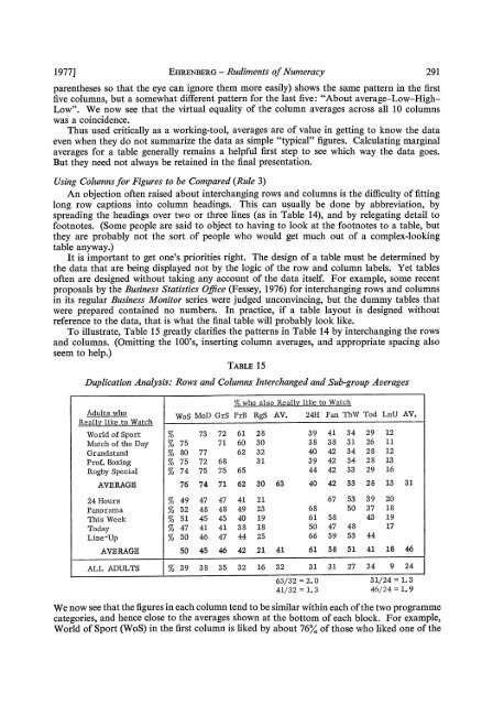
1977] EHRENBERG - Rudiments of Numeracy 291parentheseso that the eye can ignore them more easily) shows the same pattern in the firstfive columns, but a somewhat different pattern for the last five: "About average-Low-High-Low". We now see that the virtual equality of the column averages across all 10 columnswas a coincidence.Thus used critically as a working-tool, averages are of value in getting to know the dataeven when they do not summarize the data as simple "typical" figures. Calculating marginalaverages for a table generally remains a helpful first step to see which way the data goes.But they need not always be retained in the final presentation.Using Columns for Figures to be Compared (Rule 3)An objection often raised about interchanging rows and columns is the difficulty of fittinglong row captions into column headings. This can usually be done by abbreviation, byspreading the headings over two or three lines (as in Table 14), and by relegating detail tofootnotes. (Some people are said to object to having to look at the footnotes to a table, butthey are probably not the sort of people who would get much out of a complex-lookingtable anyway.)It is importanto get one's priorities right. The design of a table must be determined bythe data that are being displayed not by the logic of the row and column labels. Yet tablesoften are designed without taking any account of the data itself. For example, some recentproposals by the Business Statistics Office (Fessey, 1976) for interchanging rows and columnsin its regular Business Monitor series were judged unconvincing, but the dummy tables thatwere prepared contained no numbers. In practice, if a table layout is designed withoutreference to the data, that is what the final table will probably look like.To illustrate, Table 15 greatly clarifies the patterns in Table 14 by interchanging the rowsand columns. (Omitting the 100's, inserting column averages, and appropriate spacing alsoseem to help.)TABLE 15Duplication Analysis: Rows and Columns Interchanged and Sub-group AveragesT who also Really like to WatchAdults who WOS MoD GrS PrB RgS AV. 24H Pan ThW Tod LnU AV.Really like to WatchWorid of Sport % 73 72 61 28 39 41 34 29 12Match of the Day % 75 71 60 30 38 38 31 26 11Grandstand % 80 77 62 32 40 42 34 28 12Prof. Boxing % 75 72 68 31 39 42 34 28 13Rugby Special % 74 75 75 65 44 42 33 29 16AVERAGE 76 74 71 62 30 63 40 42 33 28 13 3124 Hours % 49 47 47 41 21 67 53 39 20Panorama % 52 48 48 49 23 68 50 37 18This Week % 51 45 45 40 19 61 58 43 19Today %T 47 41 41 38 18 50 47 48 17Line-Up % 50 46 47 44 25 66 59 53 44AVERAGE 50 45 46 42 21 41 61 58 51 41 18 46ALL ADULTS % 39 38 35 32 16 32 31 31 27 24 9 2463/32 = 2. 0 31/24 = 1. 341/32 = 1.3 46/24 = 1.9We now see that the figures in each column tend to be similar within each of the two programmecategories, and hence close to the averages shown at the bottom of each block. For example,World of Sport (WoS) in the first column is liked by about 76% of those who liked one of the
292 EHRENBERG - Rudiments of Numeracv [Part 3.other Sports programmes (the individual figures varying between 74 and 80%o), and by about50% of those who liked one of the Current Affairs programmes.Since World of Sport (WoS) is liked by about 39% of all adults (as shown in the last rowof the table), we can see now that it was about twice as popular amongst those who likedanother Sports programme, and about 1-3 times as popular amongs those who liked a CurrentAffairs programme, than amongst the population as a whole (76/39 and 50/39).The same pattern holds for the other Sports programmeshown in the next four columns(MoD to RgS). From the averages we estimate "duplication-ratios" of 63/32 = 2f0 withinthe Sports cluster and 41/32 = 1-3 between the Sports and Current Affairs programmes.The pattern also applies to the Current Affairs programmes in the last five columns of thetable. The duplication-ratios here are again 1-3 for Current Affairs versus Sports and 1-9within the Current Affairs cluster itself.Table 15 may appear more complex than the earlier correlation matrix in Table 4, but itprovides much more insight into the data. It is an instance of the so-called "duplication law",which says here that the percentage of people who like programme P amongst those who likeprogramme Q is directly proportional to the percentage of the whole population who likeprogramme P, the proportionality-factor or "duplication-ratio" being a constant for aparticular grouping of programmes. This form of relationship has already been found tooccur in a wide range of choice situations (e.g. Ehrenberg, 1972; Goodhardt et al., 1975)and also has strong theoretical backing (Goodhardt, 1966; Goodhardt et al., 1977).Table 15 may not seem obvious at a glance if one is seeing it for the firs time. But itbrings out the duplication pattern clearly enough for anyone already knowledgeable in thearea, and in particular for anyone involved in using the model in question. This typicallyinvolves examining and communicating literally hundreds of thousands of such figures overthe years. A form of layout meeting the weak criterion for a good table which allows one toscan and grasp extensive data then becomes essential.A common query about changing rows into columns is whether all users of the table willwant to compare the figures in the columns rather than those in the rows. In practice theymust always do both. But the main pattern in the data should be looked at first and hence incolumns because that is easier. Then, having seen the main pattern, one can look at the rowsand at any row-and-column interactions. Again, with a table of time-series one usually looksfirst at each series on its own (which is easier in columns) and only then correlates the differentseries.Ordering by Size (Rule 4)Ordering the rows or colunns of a table by some measure of size raises two problems.One is that different measures of size can be used, resulting in different possible orders. Thecriticism is that readers (especially othe readers) might be misled by the particular order chosen.For example, in Table 2 ordering the rows of the shipping data by the numbers of vesselsled to the sequence Cargo/Tanker/Passenger. Ordering by the 1973 tonnages would have ledto the sequence Tanker/Cargo/Passenger. But users of a table do not have to accept thechosen ordering as sacrosanct. One order will show up the conflict with another, and somevisible ordering is always better than none (as in the original Table 1). In Table 2 anyone cansee that the 1973 tonnages were out of step. (Were you, the reader, in any way misled, or wouldyou only be worrying about the possible effect on others?)The second problem arises when there are many different tables with the same basic formatand straight application of the rule would lead to different orders for different tables. In suchcases the same order should be used in every table.A good example occurs with tables giving various social and economic statistics fordifferent countries, or for different regions or towns within the same country. A usefulcommon order for all such tables might be population size. This provides an instant visualrank correlation between the absolute and per capita rates for each variable.
Page 1 and 2: Rudiments of NumeracyAuthor(s): A.
Page 3 and 4: 278 EHRENBERG - Rudiments of Numera
Page 15: 290 EHRENBERG - Rudiments of Numera

Rudiments of Numeracy by A.S.C.Ehrenberg - School of Mathematics

Create successful ePaper yourself

Delete template?

Save as template?