Mass Loss by Inhomogeneous Agb-Winds
Mass Loss by Inhomogeneous Agb-Winds
Mass Loss by Inhomogeneous Agb-Winds

You also want an ePaper? Increase the reach of your titles
YUMPU automatically turns print PDFs into web optimized ePapers that Google loves.
<strong>Mass</strong> <strong>Loss</strong> <strong>by</strong> <strong>Inhomogeneous</strong><br />
AGB-<strong>Winds</strong><br />
Detailed Structures in Planetary Nebulae<br />
Dissertation<br />
eingereicht von<br />
Mag. rer. nat. Ch. Reimers<br />
zur Erlangung des akademischen Grades<br />
Doktor der Naturwissenschaften<br />
Fakultät für Geowissenschaften,<br />
Geographie und Astronomie<br />
der Universität Wien<br />
Institut für Astronomie<br />
Türkenschanzstraße 17<br />
A-1180 Wien, Österreich<br />
Oktober 2005
Preface<br />
On the one hand the distances in the universe as well as the dimensions of astrophysical<br />
objects like galaxies are almost unimaginable. On the other hand the time<br />
scales are either immeasurably long as compared with our human being (e.g. the lifetime<br />
of a typical star like our Sun) or they are even faster than a “human thought”<br />
(e.g. the supernova explosion process, the rotation period of fast rotating pulsars or<br />
the atomic vibrational timescales). Therefore, the fascination to study astrophysical<br />
problems is the possibility to model and solve the “physical world” with the help<br />
of computer technology and specific software. This fascination was also a driving<br />
motivation for the realisation of this thesis.<br />
In order to reconstruct astrophysics here on Earth, computer simulations are inevitable,<br />
which divide the space into small units (in the broadest sense this can be<br />
denoted <strong>by</strong> spatial resolution) and arrange the time as finite intervals, which are<br />
called time steps. This procedure one calls also discretisation, which was realised<br />
<strong>by</strong> the development of a program (hereafter RHD code) to simulate radiation hydrodynamic<br />
problems at the Institute for Astronomy of the University of Vienna.<br />
The RHD code is already extensively tested <strong>by</strong> several calculations to various astronomical<br />
objects, e.g. RR Lyra stars, Cepheids, LBVs, protostellar collapse and<br />
AGB stars. Among other things the work is to be understood as an extension to<br />
this RHD code.<br />
I would like to thank my dissertation advisor, Ernst A. Dorfi, for his support and<br />
encouragement over the previous years. I benefited from his teaching of computer<br />
simulation and he led me to break through problems which certainly resulted in a<br />
timely completion of this thesis.<br />
Also many thanks to the preparatory work of the RHD code done <strong>by</strong> Susanne<br />
Höfner, Michael U. Feuchtinger as well as Ernst A. Dorfi. Furthermore, a big thank<br />
to Roland Ottensamer for proof-reading of this thesis. Finally, I acknowledge the discussions,<br />
inspirations and patience of all the students and combatants, who worked<br />
in the same computer working room as me.<br />
Vienna, October 2005 Mag. Christian Reimers
Abstract<br />
AGB (Asymptotic Giant Branch) stars generate a massive dust driven stellar wind at<br />
the end of their lives. There<strong>by</strong> they lose a large amount of mass. Ideally, this mass<br />
loss is spherical if the physical conditions are homogeneous at the stellar surface<br />
(e.g. temperature) and the stellar vicinity (e.g. density). Indeed, several physical<br />
processes induce deviations from these ideal conditions. A stellar rotation for example<br />
generates an asphericity of the luminosity or alternatively effective temperature<br />
at the stellar photosphere. This will affect the condensation of dust and therefore<br />
the mass loss rate. The dust formation process depends strongly on the temperature<br />
and density.<br />
Inhomogeneities can also caused <strong>by</strong> cool spots at the stellar surface. For some<br />
time it is known that spots are common on stars and are much often larger than<br />
spots on our Sun. These inhomogeneities of the temperature are able to emanate<br />
from a magnetic field or a huge convection cell within the stellar envelope. Both<br />
options are possible at the surface of AGB-stars. Due to the massive dust formation<br />
in their atmospheres these physical processes are difficult to observe. But several<br />
theoretical calculations and investigations are able to support such a theory.<br />
This thesis introduces a model for the investigation of the mass loss above cool<br />
spots. For that purpose a radiation hydrodynamic simulation (including a gas, a dust<br />
and a radiation component) has been used and modified for the special purposes of<br />
this problem. A flux tube geometry has been chosen which could have been produced<br />
<strong>by</strong> a magnetic field in the lower stellar atmosphere. Finally, a discussion has been<br />
carried out about the creation of dense knots in planetary nebula as a result of<br />
cool regions at the stellar surface. A large amount of those dense knots or cometary<br />
structures can be observed in many planetary nebula, like in the Helix or the Eskimo<br />
Nebula.<br />
The result supports the theory that stellar spots generate significant inhomogeneities<br />
of the mass loss. But the formation of dense knots in planetary nebulae<br />
have to be interpreted as a combination of inhomogeneities in the mass loss together<br />
with hydrodynamical instabilities. The model investigated describes the formation<br />
of initial inhomogeneities which can be later amplified <strong>by</strong> an interaction of the slow<br />
AGB wind with the fast tenuous wind of the hot central star of the planetary nebula.
Zusammenfassung<br />
AGB-Sterne (Asymptotic Giant Branch) produzieren am Ende ihres Lebens einen<br />
ausgeprägten staubgetriebenen Sternwind, bei dem sie einen Großteil ihrer Hüllenmasse<br />
verlieren. Idealerweise ist dieser <strong>Mass</strong>enverlust sphärisch symmetrisch, wenn<br />
die physikalischen Größen an der Sternoberfläche (z.B. Temperatur) und im umgebenden<br />
Medium (z.B. Dichte) homogen sind. Allerdings erzeugen verschiedene<br />
physikalische Prozesse Abweichungen von diesen idealen Bedingungen. Zum Beispiel<br />
bewirkt die Rotation des Sterns eine Aspherizität der Sternleuchtkraft beziehungsweise<br />
Effektivtemperatur an der Sternphotosphäre, welche sich auf die Kondensation<br />
des Staubs und daraus folgend auf die <strong>Mass</strong>enverlustrate auswirkt. Der Staubentstehungsprozess<br />
ist stark von Temperatur und Dichte abhängig.<br />
Inhomogenitäten können auch durch kühle Flecken auf der Sternoberfläche erzeugt<br />
werden. Schon seit einiger Zeit ist bekannt, dass es Sterne mit Flecken gibt, die<br />
mitunter einiges größer sind als Sonnenflecken. Diese Temperaturinhomogenitäten<br />
können von einem Magnetfeld oder aber von großräumigen Konvektionszellen in<br />
einer konvektiven äußeren Hülle stammen. Beide Möglichkeiten sind für die Oberfläche<br />
von AGB-Sternen vorstellbar. Beobachtungen diesbezüglich sind wegen der<br />
hohen Staubproduktion in den AGB-Atmosphären nur schwer zu machen. Verschiedene<br />
Modellrechnungen und theoretische Überlegungen unterstützen jedoch<br />
diese Theorie.<br />
In dieser Arbeit wird ein Modell vorgestellt, das zur Untersuchung des <strong>Mass</strong>enverlustes<br />
über diskreten kühlen Flecken dient. Dazu kam eine strahlungshydrodynamische<br />
Simulation zum Einsatz, die eine Gas-, Staub- und Strahlungs-Komponente<br />
beinhaltet, wobei der Computer-Code für die neue Applikation adaptiert werden<br />
musste. Um den komplexen Sachverhalt zu vereinfachen wurde eine Flussröhren-<br />
Geometrie gewählt, die ein Magnetfeld in der unteren Sternatmosphäre erzeugt.<br />
Eine abschließende Diskussion soll klären, ob diese kühlen Regionen auf der Sternoberfläche<br />
die Existenz von dichten Knoten in Planetarischen Nebeln hervorrufen<br />
kann. In vielen Planetarischen Nebeln sind wir in der Lage eine große Anzahl dichter<br />
Knoten oder “kometenartiger” Strukturen zu beobachten (z.B. im Helix- oder im<br />
Eskimo-Nebel).<br />
Das Ergebnis unterstützt die Theorie, dass Sternflecken eine signifikante Inhomogenität<br />
im <strong>Mass</strong>enverlust verursachen können. Allerdings müssen die beobachteten<br />
dichten Knoten in Planetarischen Nebeln in Verbindung mit hydrodynamischen<br />
Instabilitäten entstanden sein. Das untersuchte Modell erzeugt dabei eine anfängliche<br />
Inhomogenität im stellaren Ausfluss, welche später durch die Wechselwirkung des<br />
langsamen AGB-Windes mit dem schnellen dünnen Wind des heißen Zentralsterns<br />
Planetarischer Nebel verstärkt werden kann.
Contents<br />
I Introduction and Motivation 1<br />
1 Evolution of Stars 3<br />
1.1 The Cycle of Matter . . . . . . . . . . . . . . . . . . . . . . . . . . . 3<br />
1.1.1 Interstellar Medium . . . . . . . . . . . . . . . . . . . . . . . 3<br />
1.1.2 Exchange of Matter . . . . . . . . . . . . . . . . . . . . . . . 4<br />
1.2 Stellar Evolution . . . . . . . . . . . . . . . . . . . . . . . . . . . . . 4<br />
1.2.1 Star Formation . . . . . . . . . . . . . . . . . . . . . . . . . . 4<br />
1.2.2 Constant Light of Hydrogen Fusion - The Main Sequence . . 5<br />
1.2.3 Final Stages of Stars . . . . . . . . . . . . . . . . . . . . . . . 5<br />
1.3 Origin and Composition of Stellar Dust . . . . . . . . . . . . . . . . 7<br />
1.3.1 Properties of AGB stars . . . . . . . . . . . . . . . . . . . . . 7<br />
1.3.2 Detecting and Measuring Interstellar Dust Grains . . . . . . 9<br />
1.3.3 Dust Formation and Destruction . . . . . . . . . . . . . . . . 10<br />
1.4 From AGB stars to PNe . . . . . . . . . . . . . . . . . . . . . . . . . 11<br />
2 Planetary Nebulae 13<br />
2.1 Morphology and Classification . . . . . . . . . . . . . . . . . . . . . . 13<br />
2.1.1 List of Prominent PNe . . . . . . . . . . . . . . . . . . . . . . 14<br />
2.2 Examples . . . . . . . . . . . . . . . . . . . . . . . . . . . . . . . . . 15<br />
2.2.1 Proto-PNe (or Young PNe) . . . . . . . . . . . . . . . . . . . 15<br />
2.2.2 Round and Elliptical . . . . . . . . . . . . . . . . . . . . . . . 18<br />
2.2.3 Bipolar and Quadrupolar . . . . . . . . . . . . . . . . . . . . 25<br />
2.3 Global Models to Shape a PN . . . . . . . . . . . . . . . . . . . . . . 29<br />
2.3.1 Multiple-<strong>Winds</strong> Model . . . . . . . . . . . . . . . . . . . . . . 29<br />
2.3.2 Aspherical <strong>Mass</strong> <strong>Loss</strong> of AGB stars . . . . . . . . . . . . . . . 29<br />
2.3.3 The Role of Magnetic Fields . . . . . . . . . . . . . . . . . . 30<br />
2.3.4 Interaction with the ISM . . . . . . . . . . . . . . . . . . . . 31<br />
2.3.5 MHD Models . . . . . . . . . . . . . . . . . . . . . . . . . . . 31<br />
2.4 Details in PNe . . . . . . . . . . . . . . . . . . . . . . . . . . . . . . 32<br />
2.4.1 Halo . . . . . . . . . . . . . . . . . . . . . . . . . . . . . . . . 32<br />
2.4.2 Jets, Lobes and Ansae . . . . . . . . . . . . . . . . . . . . . . 33<br />
2.4.3 Knots . . . . . . . . . . . . . . . . . . . . . . . . . . . . . . . 33<br />
v
vi CONTENTS<br />
II Theoretical Models 35<br />
3 Radiation Hydrodynamics Simulation 37<br />
3.1 Basic Equations . . . . . . . . . . . . . . . . . . . . . . . . . . . . . . 37<br />
3.1.1 Conservation form . . . . . . . . . . . . . . . . . . . . . . . . 37<br />
3.1.2 Gas Component . . . . . . . . . . . . . . . . . . . . . . . . . 38<br />
3.1.3 Radiation Field . . . . . . . . . . . . . . . . . . . . . . . . . . 40<br />
3.1.4 Dust . . . . . . . . . . . . . . . . . . . . . . . . . . . . . . . . 41<br />
3.2 Additional Equations and Constitutive Relations . . . . . . . . . . . 42<br />
3.2.1 Grid Equation . . . . . . . . . . . . . . . . . . . . . . . . . . 42<br />
3.2.2 <strong>Mass</strong> Equation . . . . . . . . . . . . . . . . . . . . . . . . . . 42<br />
3.2.3 Poisson Equation . . . . . . . . . . . . . . . . . . . . . . . . . 43<br />
3.2.4 Equation of State (EOS) . . . . . . . . . . . . . . . . . . . . . 43<br />
3.2.5 Opacity of Gas and Dust . . . . . . . . . . . . . . . . . . . . 44<br />
3.2.6 Source Function of Gas and Dust . . . . . . . . . . . . . . . . 45<br />
3.2.7 Eddington Factor . . . . . . . . . . . . . . . . . . . . . . . . . 45<br />
3.3 Boundary Conditions . . . . . . . . . . . . . . . . . . . . . . . . . . . 46<br />
3.3.1 Inner Boundary . . . . . . . . . . . . . . . . . . . . . . . . . . 46<br />
3.3.2 Outer Boundary . . . . . . . . . . . . . . . . . . . . . . . . . 46<br />
3.4 Initial Models . . . . . . . . . . . . . . . . . . . . . . . . . . . . . . . 47<br />
3.4.1 Modelling Method . . . . . . . . . . . . . . . . . . . . . . . . 47<br />
3.4.2 Equations for the Stellar Envelope . . . . . . . . . . . . . . . 49<br />
3.4.3 Equations for the Stellar Atmosphere . . . . . . . . . . . . . 50<br />
3.4.4 Additional Notes . . . . . . . . . . . . . . . . . . . . . . . . . 52<br />
3.5 Numerical Methods . . . . . . . . . . . . . . . . . . . . . . . . . . . . 53<br />
4 Stellar Spots 55<br />
4.1 Introduction . . . . . . . . . . . . . . . . . . . . . . . . . . . . . . . . 55<br />
4.1.1 Solar Magnetic Activity and Sunspots . . . . . . . . . . . . . 55<br />
4.1.2 Stellar Magnetic Activity . . . . . . . . . . . . . . . . . . . . 56<br />
4.1.3 Observations of Stellar Spots . . . . . . . . . . . . . . . . . . 57<br />
4.1.4 AGB star spots . . . . . . . . . . . . . . . . . . . . . . . . . . 59<br />
4.2 Physical Model . . . . . . . . . . . . . . . . . . . . . . . . . . . . . . 60<br />
4.2.1 Spot Coverage . . . . . . . . . . . . . . . . . . . . . . . . . . 60<br />
4.2.2 Temperature Fluctuations . . . . . . . . . . . . . . . . . . . . 61<br />
4.2.3 Magnetic Field . . . . . . . . . . . . . . . . . . . . . . . . . . 61<br />
4.2.4 Dust Formation above Cool Spots . . . . . . . . . . . . . . . 62<br />
4.3 Flux Tube Model . . . . . . . . . . . . . . . . . . . . . . . . . . . . . 63<br />
4.3.1 Definition . . . . . . . . . . . . . . . . . . . . . . . . . . . . . 63<br />
4.3.2 Flux Tube Representations . . . . . . . . . . . . . . . . . . . 63
CONTENTS vii<br />
4.3.3 Specific Declarations and Boundary Conditions . . . . . . . . 67<br />
4.3.4 Rewritten Equations . . . . . . . . . . . . . . . . . . . . . . . 68<br />
III Results and Discussion 71<br />
5 AGB Stars with Spots 73<br />
5.1 Initial Models . . . . . . . . . . . . . . . . . . . . . . . . . . . . . . . 73<br />
5.1.1 Initial Models for Spherical Geometry . . . . . . . . . . . . . 73<br />
5.1.2 Initial Models for Flux Tube Geometry . . . . . . . . . . . . 76<br />
5.2 Dynamic Model Results for Spherical Geometry . . . . . . . . . . . . 79<br />
5.2.1 Effects of Chemistry . . . . . . . . . . . . . . . . . . . . . . . 81<br />
5.3 Dynamic Model Results for Flux Tube Geometry . . . . . . . . . . . 82<br />
5.3.1 Effects of Geometry . . . . . . . . . . . . . . . . . . . . . . . 85<br />
5.4 Boundary Conditions of the Flux Tube . . . . . . . . . . . . . . . . . 88<br />
5.4.1 Lateral Pressure . . . . . . . . . . . . . . . . . . . . . . . . . 88<br />
5.4.2 Heat Sources and Sinks . . . . . . . . . . . . . . . . . . . . . 90<br />
5.5 <strong>Mass</strong> <strong>Loss</strong> through a Flux Tube . . . . . . . . . . . . . . . . . . . . . 91<br />
6 Discussion and Perspectives 95<br />
6.1 Magnetic Field . . . . . . . . . . . . . . . . . . . . . . . . . . . . . . 95<br />
6.1.1 Lifetime of Stellar Spots . . . . . . . . . . . . . . . . . . . . . 95<br />
6.1.2 Stellar Activity Cycle . . . . . . . . . . . . . . . . . . . . . . 97<br />
6.1.3 Size and Distribution of Stellar Spots . . . . . . . . . . . . . 97<br />
6.2 <strong>Mass</strong> <strong>Loss</strong> . . . . . . . . . . . . . . . . . . . . . . . . . . . . . . . . . 97<br />
6.2.1 <strong>Mass</strong> Acquiration . . . . . . . . . . . . . . . . . . . . . . . . . 97<br />
6.2.2 Stellar Rotation . . . . . . . . . . . . . . . . . . . . . . . . . 98<br />
6.3 Small-scale Structures in PNe . . . . . . . . . . . . . . . . . . . . . . 99<br />
6.3.1 Instabilities . . . . . . . . . . . . . . . . . . . . . . . . . . . . 99<br />
6.3.2 <strong>Inhomogeneous</strong> <strong>Mass</strong> <strong>Loss</strong> . . . . . . . . . . . . . . . . . . . . 99<br />
6.3.3 Radial Filaments . . . . . . . . . . . . . . . . . . . . . . . . . 100<br />
6.4 Conclusion . . . . . . . . . . . . . . . . . . . . . . . . . . . . . . . . 100<br />
6.5 Assumptions and further Perspectives . . . . . . . . . . . . . . . . . 101<br />
6.5.1 Geometry . . . . . . . . . . . . . . . . . . . . . . . . . . . . . 101<br />
6.5.2 Magnetic Field . . . . . . . . . . . . . . . . . . . . . . . . . . 101<br />
6.5.3 Permeable Boundary . . . . . . . . . . . . . . . . . . . . . . . 101<br />
6.5.4 Stellar Pulsations . . . . . . . . . . . . . . . . . . . . . . . . . 102
viii CONTENTS<br />
IV Appendices 103<br />
A Discretisation 105<br />
A.1 Computational Domain . . . . . . . . . . . . . . . . . . . . . . . . . 105<br />
A.2 Rules . . . . . . . . . . . . . . . . . . . . . . . . . . . . . . . . . . . . 105<br />
A.3 General . . . . . . . . . . . . . . . . . . . . . . . . . . . . . . . . . . 106<br />
A.4 Case 1: Spherical Geometry . . . . . . . . . . . . . . . . . . . . . . . 106<br />
A.4.1 Advection . . . . . . . . . . . . . . . . . . . . . . . . . . . . . 106<br />
A.4.2 Mathematical Operators . . . . . . . . . . . . . . . . . . . . . 107<br />
A.5 Case 2: Flux Tube Geometry . . . . . . . . . . . . . . . . . . . . . . 107<br />
A.5.1 Advection . . . . . . . . . . . . . . . . . . . . . . . . . . . . . 107<br />
A.5.2 Mathematical Operators . . . . . . . . . . . . . . . . . . . . . 107<br />
B Artificial Viscosity 109<br />
B.1 General . . . . . . . . . . . . . . . . . . . . . . . . . . . . . . . . . . 109<br />
B.1.1 Viscous Force . . . . . . . . . . . . . . . . . . . . . . . . . . . 110<br />
B.1.2 Viscous Energy Dissipation . . . . . . . . . . . . . . . . . . . 110<br />
B.2 Case 1: Spherical Geometry . . . . . . . . . . . . . . . . . . . . . . . 111<br />
B.2.1 Results . . . . . . . . . . . . . . . . . . . . . . . . . . . . . . 112<br />
B.2.2 Discretisation . . . . . . . . . . . . . . . . . . . . . . . . . . . 112<br />
B.3 Case 2: Flux Tube Geometry . . . . . . . . . . . . . . . . . . . . . . 113<br />
B.3.1 Results . . . . . . . . . . . . . . . . . . . . . . . . . . . . . . 114<br />
B.3.2 Discretisation . . . . . . . . . . . . . . . . . . . . . . . . . . . 114<br />
C Radiation Transfer 115<br />
C.1 Radiation Transfer Equation . . . . . . . . . . . . . . . . . . . . . . 115<br />
C.1.1 General . . . . . . . . . . . . . . . . . . . . . . . . . . . . . . 115<br />
C.1.2 RTE in General Geometry . . . . . . . . . . . . . . . . . . . . 115<br />
C.1.3 Variables and Moments . . . . . . . . . . . . . . . . . . . . . 119<br />
C.1.4 Radiation Pressure Tensor Identities . . . . . . . . . . . . . . 119<br />
C.2 0 th -order Moment Equation . . . . . . . . . . . . . . . . . . . . . . . 121<br />
C.2.1 Case 1: Spherical Geometry . . . . . . . . . . . . . . . . . . . 121<br />
C.2.2 Case 2: Flux Tube Geometry . . . . . . . . . . . . . . . . . . 122<br />
C.3 1 st -order Moment Equation . . . . . . . . . . . . . . . . . . . . . . . 123<br />
C.3.1 Case 1: Spherical Geometry . . . . . . . . . . . . . . . . . . . 123<br />
C.3.2 Case 2: Flux Tube Geometry . . . . . . . . . . . . . . . . . . 124<br />
C.4 Derivatives in different geometries . . . . . . . . . . . . . . . . . . . 124<br />
C.5 Summary of Spherical Radiation Equations . . . . . . . . . . . . . . 125<br />
C.5.1 Radiation Energy Equation . . . . . . . . . . . . . . . . . . . 125<br />
C.5.2 Radiation Momentum Equation . . . . . . . . . . . . . . . . . 126
CONTENTS ix<br />
D Dust properties 127<br />
D.1 Constants . . . . . . . . . . . . . . . . . . . . . . . . . . . . . . . . . 127<br />
D.2 Variables . . . . . . . . . . . . . . . . . . . . . . . . . . . . . . . . . 127<br />
D.3 Dust Formation . . . . . . . . . . . . . . . . . . . . . . . . . . . . . . 128<br />
D.3.1 C-rich Chemistry . . . . . . . . . . . . . . . . . . . . . . . . . 128<br />
D.3.2 Nucleation Theory . . . . . . . . . . . . . . . . . . . . . . . . 131<br />
D.3.3 Dust Physics . . . . . . . . . . . . . . . . . . . . . . . . . . . 134<br />
E Tensor Calculus 135<br />
E.1 General . . . . . . . . . . . . . . . . . . . . . . . . . . . . . . . . . . 135<br />
E.1.1 Historical Background . . . . . . . . . . . . . . . . . . . . . . 135<br />
E.1.2 Definitions . . . . . . . . . . . . . . . . . . . . . . . . . . . . 135<br />
E.2 Vectors . . . . . . . . . . . . . . . . . . . . . . . . . . . . . . . . . . 137<br />
E.2.1 Definitions . . . . . . . . . . . . . . . . . . . . . . . . . . . . 137<br />
E.2.2 Operations and Operators . . . . . . . . . . . . . . . . . . . . 138<br />
E.2.3 Relations / Vector Identities . . . . . . . . . . . . . . . . . . 141<br />
E.3 Tensors . . . . . . . . . . . . . . . . . . . . . . . . . . . . . . . . . . 142<br />
E.3.1 Definitions . . . . . . . . . . . . . . . . . . . . . . . . . . . . 142<br />
E.3.2 Operations and Operators . . . . . . . . . . . . . . . . . . . . 142<br />
E.3.3 Relations / Tensor Identities . . . . . . . . . . . . . . . . . . 144<br />
E.4 Metric and Symmetries . . . . . . . . . . . . . . . . . . . . . . . . . 145<br />
E.4.1 Metric . . . . . . . . . . . . . . . . . . . . . . . . . . . . . . . 145<br />
E.4.2 Coordinate Systems . . . . . . . . . . . . . . . . . . . . . . . 147<br />
F Full Set of RHD Equations 153<br />
F.1 Differential Form . . . . . . . . . . . . . . . . . . . . . . . . . . . . . 154<br />
F.2 Integrated Form . . . . . . . . . . . . . . . . . . . . . . . . . . . . . 155<br />
F.3 Discretised Form . . . . . . . . . . . . . . . . . . . . . . . . . . . . . 157<br />
G Symbols, Constants and Abbreviations 159<br />
G.1 Symbols . . . . . . . . . . . . . . . . . . . . . . . . . . . . . . . . . . 159<br />
G.2 Fundamental Physical Constants . . . . . . . . . . . . . . . . . . . . 160<br />
G.3 Astronomical Constants . . . . . . . . . . . . . . . . . . . . . . . . . 160<br />
G.4 Abbreviations . . . . . . . . . . . . . . . . . . . . . . . . . . . . . . . 161<br />
List of Tables 163<br />
List of Figures 165<br />
Image Credits 167<br />
Bibliography 169
Part I<br />
Introduction and Motivation<br />
1
Chapter 1<br />
Evolution of Stars<br />
The aim of this thesis is to investigate an inhomogeneous mass loss of asymptotic<br />
giant branch stars (hereafter AGB stars). An effective mechanism of mass loss for<br />
these cool stars is the generation of a dust driven stellar wind where the radiation<br />
pressure accelerates the newly formed dust grains. The first chapter gives a brief<br />
summary of the formation and evolution of stellar objects with special regard to<br />
intermediate mass stars like the AGB’s. In the second chapter we describe in detail<br />
the morphology and classification of planetary nebulae (hereafter PNe) with respect<br />
to the generation of models for the explanation of small-scale structures in PNe as<br />
a result of an interaction from the massive mass loss of the AGB progenitor and<br />
the high velocity outflows of the hot central objects. At first we discuss the cycle of<br />
matter in a galactical context. Therein the interstellar medium plays an important<br />
role as origin of the stellar formation process. Furthermore, an enrichment of heavy<br />
elements <strong>by</strong> the incorporation of nuclear processed material (e.g. AGB wind) leads<br />
to a chemical evolution of stellar objects.<br />
1.1 The Cycle of Matter<br />
1.1.1 Interstellar Medium<br />
The space between the stars in a galaxy is far from being empty. These regions<br />
are filled with gas, dust, solid bodies (like asteroids or comets), magnetic fields and<br />
charged particles and commonly noted as interstellar medium (hereafter ISM). Approximately<br />
99% of the mass of the ISM is in the gaseous form and the remaining 1%<br />
is composed primarily of dust. The matter of the ISM is not distributed uniformly<br />
but is more or less concentrated in interstellar clouds where complex molecules and interstellar clouds<br />
dust particles can be formed. On the one hand the molecules are the seed for the<br />
dust formation process, on the other hand they are at risk to be destroyed <strong>by</strong> the<br />
interstellar ultraviolet radiation. But in dense clouds they are shielded against this<br />
destructive radiation.<br />
Apart from molecular cloud cores dust particles are formed in several other<br />
astrophysical environments, ranging from stellar outflows (including red giant at- stellar outflows<br />
mospheres and Wolf-Rayet winds) to interstellar shock fronts and explosive ejecta<br />
(e.g. supernovae). These processes are also responsible for the chemical evolution<br />
3
4 1. EVOLUTION OF STARS<br />
dust component<br />
circulation process<br />
Jeans mass<br />
protostellar object<br />
of the ISM <strong>by</strong> the enrichment of heavy elements. The dust component of the ISM<br />
becomes detectable as (cf. Savage & Mathis 1979 [134]):<br />
• Interstellar extinction and reddening: It is caused <strong>by</strong> the absorption of light <strong>by</strong><br />
matter between the object and the observer and depends on the wavelength like<br />
Fλ ≈ λ −1 . Thus dense clouds which are opaque in visual light get transparent<br />
for higher λ (e.g. infrared radiation).<br />
• Reflection nebulae: The light from some stars embedded in an interstellar<br />
nebula is scattered <strong>by</strong> gas and dust particles therein.<br />
• Polarisation: Stellar light can become polarised when passing through a dust<br />
cloud if the particles are small compared to the incident wavelength, if they<br />
are extended in length or if they tend to be orientated in the same direction.<br />
• Infrared emission: Stellar radiation and collisions with atoms also heats up the<br />
dust in the stellar vicinity. The absorbed energy is thermalised and as a result<br />
the dust emits a thermal spectrum predominantly in the infrared wavelengths.<br />
Dust can be studied in situ within our Solar System with several methods (see<br />
therefore Section 1.3.2 on page 9).<br />
1.1.2 Exchange of Matter<br />
The ISM is constantly subject to a circulation process. The gas and dust input<br />
to the ISM is provided <strong>by</strong> supernova remnants, stellar winds and jets, whereas the<br />
losses are due to star formation and accretion on stellar objects (e.g. white dwarfs,<br />
neutron stars, etc.). The ISM matter is lost forever, when it gets trapped <strong>by</strong> stellar<br />
or galactic black holes.<br />
1.2 Stellar Evolution<br />
1.2.1 Star Formation<br />
The starting point of star formation is gas and dust concentrated in interstellar<br />
molecular clouds. Dynamical processes like shock waves from energetic events in<br />
the surrounding, e.g. supernova explosions, can trigger the gravitational collapse. If<br />
enough matter is concentrated, the gravitational force dominates the counteracting<br />
pressure forces, i.e. the mass concentration rises above the Jeans mass<br />
Mj ∝ ρ −1<br />
2 T 3<br />
2 (1.1)<br />
(since Jeans first demonstrated the nature of this instability in 1902, it is called<br />
Jeans instability and the involved mass is called Jeans mass), the collapse acts in<br />
and fragmentation may reduce the initial mass. The collapse to a protostellar object<br />
needs between 10 4 and 10 6 years.
1.2. Stellar Evolution 5<br />
Depending on the mass involved, stars with main sequence masses in the<br />
• low (0.08 � M[M⊙] � 2),<br />
• intermediate (2 � M[M⊙] � 8) or<br />
• high (M[M⊙] � 8)<br />
mass range can be formed. After the formation of single or double stars the initial<br />
mass remains mostly constant. But if two or more stars orbit each other closely, the mass transfer<br />
gravitational forces can transfer stellar matter from one star to its companion. This<br />
mass transfer has an impact on the further evolution of each star.<br />
Furthermore, remaining matter from stellar formation generates a disc orbiting<br />
the protostellar object. Matter bound in these stellar accretion discs can be the accretion disc<br />
seed for the formation of huge layered grains, clumps and further for planetesimals.<br />
If the conditions are favourable then asteroids, moons and finally planets emanates<br />
from these building components.<br />
1.2.2 Constant Light of Hydrogen Fusion - The Main Sequence<br />
Single stars with masses less than 1.4 M⊙ remain at the main-sequence (hereafter<br />
MS) stage for a very long period. The MS lifetime of a star can be estimated <strong>by</strong> the main sequence<br />
nuclear timescale<br />
τnuc ∼<br />
available fuel<br />
burning rate<br />
∼ M<br />
L ∼ M −2.5 , (1.2)<br />
where L is the stellar luminosity and for a MS star L ∝ M 3.5 . Due to fusion hydrogen fusion<br />
hydrogen is converted into helium in the stellar core. During this time the chemical<br />
composition of the star changes and the central temperature slowly rises. For single<br />
stars more massive than the Sun, the nuclear timescale (cf. Eq. (1.2)) decreases and<br />
the MS phase gets shorter.<br />
1.2.3 Final Stages of Stars<br />
The final stages depend on the initial masses of stars and the amount of mass which<br />
is stripped <strong>by</strong> mass loss due to companion stars or stellar winds. The following mass loss<br />
remnants left over from these stages ordered <strong>by</strong> the mass at the MS:<br />
• White Dwarfs,<br />
• Neutron Stars and<br />
• Black Holes.<br />
At the end typical masses for White Dwarfs are 0.6M⊙ and for Neutron Stars<br />
around 1.4M⊙.<br />
Low <strong>Mass</strong> Stars<br />
According to Eq. (1.2) small and relatively cool stars, which are also called red<br />
dwarfs, stay for a long time on the MS compared to stars in the higher mass ranges. red dwarf stars<br />
The masses of red dwarfs are less than about 0.5M⊙ down to objects with 0.08M⊙.<br />
Below this mass range a stellar object never gets hot enough to initiate hydrogen<br />
fusion in the core.
6 1. EVOLUTION OF STARS<br />
red giant branch<br />
hydrogen burning<br />
shell<br />
helium fusion<br />
asymptotic giant<br />
branch<br />
long period<br />
variables<br />
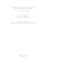
Figure 1.1: Evolutionary tracks in the Hertzsprung-Russell-Diagram for stars with<br />
initial masses of 1M⊙, 5M⊙ and 25M⊙. It shows major phases of the stellar evolution<br />
like the core helium flash, thermal pulses and the ejection of the planetary nebula<br />
(from Iben 1985 [73]).<br />
Intermediate Stars<br />
When the hydrogen fuel is exhausted in the centre of a star within an intermediate<br />
mass range of 1 to 8 M⊙ it leaves the main-sequence phase and evolves towards<br />
the so-called red giant branch (RGB). While the star itself expands the remaining<br />
hydrogen fusion in a shell around the helium rich centre generates energy for fur-<br />
ther million years. The stellar core contracts and pressure and temperature increase<br />
until the helium fusion in the stellar centre begins. Now the evolution proceeds<br />
very rapidly and the star is now located on the asymptotic giant branch (AGB) in<br />
the Hertzsprung-Russell-Diagram or short HRD (cf. Fig. 1.1). AGB stars are very<br />
extended objects with radii of a few hundred R⊙ with high luminosities of about<br />
10 3 to a few 10 4 L⊙ and low effective temperatures of typically < 3500 K. During<br />
their evolution along the AGB they begin to pulsate with large amplitudes, get large<br />
convection zones and drive a massive stellar wind. According to the noticeable pulsations<br />
with long periods the stars are also commonly known as long period variables
1.3. Origin and Composition of Stellar Dust 7<br />
(for a more detailed classification see Sect. 1.3.1). These long period pulsations are<br />
known for a long time. The first observations were made <strong>by</strong> the discoverer of Mira,<br />
David Fabricius in 1596 and 1609. The Mira stars show variations of their visual Mira stars<br />
light curves with amplitudes of several magnitudes and periods of approximately<br />
one year. The pulsations and the stellar mass loss are an observational evidence<br />
of dynamical processes these stars undergo. Later they reach the post-AGB phase post-AGB<br />
and the repelled outer envelope can be seen for about 10 5 years as PNe whilst the<br />
central object cools to a White Dwarf. More about this type of final stage will be White Dwarf<br />
given in Section 1.3 and Section 1.4.<br />
<strong>Mass</strong>ive Stars<br />
These stars can continue generating energy <strong>by</strong> helium fusion after they have<br />
depleted their hydrogen supplies. Their gravitational potential energy enables them<br />
to build up extremely high pressures and temperatures deep in their interior. These<br />
conditions are able to initiate the fusion of helium and further heavier elements.<br />
After a short red giant phase massive stars mostly end their lives in a gigantic heavy elements<br />
explosion, a supernova, leaving behind a Neutron Star or a Black Hole. Although supernovae<br />
this basic picture is supported <strong>by</strong> observations, the details of the formation process<br />
of Neutron Stars, e.g. as rapidly rotating pulsars, or even Black Holes, still remains<br />
unclear.<br />
1.3 Origin and Composition of Stellar Dust<br />
AGB stars are known to eject much of their envelope into space and this could be<br />
a significant source of interstellar dust grains (e.g. Nittler et al. 1997 [107]). Such<br />
stars have once been like the Sun but have reached a period in their life-cycle where<br />
they are losing massive amounts of dust and gas preceding their final existence as<br />
White Dwarfs.<br />
1.3.1 Properties of AGB stars<br />
Internal Structure and Nucleosynthesis<br />
The core of an AGB star consists mainly of carbon and oxygen after the central<br />
helium fusion has exhausted. Above this core a helium- and hydrogen-burning shell<br />
converts the atomic binding energies into radiation and heavier elements like carbon helium- and<br />
and oxygen, which enrich the core <strong>by</strong> mass with these heavy elements. Due to<br />
the highly degenerated electrons, the outward diffusion of the energy <strong>by</strong> electron<br />
conduction is very efficient. Furthermore, the inner part of the core loses energy<br />
<strong>by</strong> the production of neutrinos. Consequently, the temperature of the core can not<br />
climb over the temperature where carbon-burning ignites.<br />
hydrogenburning<br />
shell<br />
Theoretical models tell us that the observed peculiarities on their surfaces are<br />
directly connected with the nucleosynthesis in the stellar interior. Newly formed<br />
elements like carbon and oxygen are mixed to the surface <strong>by</strong> a deep convection zone<br />
(in particular during the so-called the third dredge-up). These mixing processes third dredge-up<br />
occur during the thermal pulsing phase (cf. TP-AGB on page 11) which involves also<br />
the external layers (Iben 1981[74]). Observations show two main types of AGB stars
8 1. EVOLUTION OF STARS<br />
surface composition<br />
long period<br />
variables<br />
κ-mechanism<br />
convection zone<br />
mixing<br />
convection cell<br />
α Orionis<br />
(Beteigeuze)<br />
infrared excess<br />
terminal wind<br />
velocities<br />
concerning their surface composition: oxygen-rich (i.e. stars with surface abundances<br />
of ǫC/ǫO < 1) and carbon-rich (i.e. ǫC/ǫO > 1) AGB stars. Due to the possible<br />
evolution from oxygen-rich stars and the effects of the third dredge-up the formation<br />
to the carbon-rich stars can be explained.<br />
Pulsation and Variability<br />
A large fraction of the AGB stars shows variability with periods of about 80 to<br />
1000 days, which are consequently called long period variables (hereafter LPVs).<br />
The LPVs are divided into several groups according to the regularity of their light<br />
curves:<br />
• Miras showing well defined periods and rather regular shapes,<br />
• semi-regular (SR) with semi-regular light curves and smaller amplitudes<br />
compared to Mira variables (for e.g. classification and evolutionary status of<br />
SR variables see Kerschbaum & Hron 1992 [82]) and<br />
• irregular variables which show no regularity in their light curves.<br />
Light curves of such stars can be found e.g. in Querci & Querci (1986 [120]). The<br />
variability of the LPVs can be explained as a radial pulsation with large amplitudes<br />
caused <strong>by</strong> a κ-mechanism in the hydrogen- and helium-ionisation zones.<br />
Convection<br />
Convection plays an important role for the transport of energy and momentum<br />
throughout most of the outer parts of the star. During the RGB phase the convection<br />
zone moves inward. This causes a mixing of nuclear processed gas upwards. The<br />
mixing to the surface of the star is called dredge-up and can change the surface<br />
composition (Iben 1985 [73]). Schwarzschild (1975 [138]) has estimated the sizes<br />
of the convective elements (scale of the dominant convection or convection cell) for<br />
Red Giant stars. Only few large convection cells should appear at the photosphere.<br />
Observations e.g. of α Orionis (Beteigeuze) (Gilliland & Dupree 1996 [54]) and three-<br />
dimensional MHD-simulations (e.g. Dorch 2004 [35], Freytag 2003 [45] and Freytag<br />
et al. 2002 [46]) also support the fact of large convection cells.<br />
Circumstellar Envelope and <strong>Mass</strong> <strong>Loss</strong><br />
From the observation of a so-called infrared excess the presence of a circumstellar<br />
envelope (hereafter CSE) around an AGB star can be inferred as done <strong>by</strong> IRAS<br />
observations (e.g. Likkel et al. 1990 [90]). The infrared excess is explained <strong>by</strong> the<br />
absorption of photospheric radiation <strong>by</strong> the CSE, thermalisation and re-emission at<br />
longer wavelengths.<br />
The observation of line profiles in the spectra of CSEs shows also expanding<br />
material where the terminal wind velocities of typically 10 to 40 km/s have been<br />
measured. This observed velocities are relatively small and below the escape velocities<br />
near the stellar photosphere indicating that the mechanism for driving the AGB<br />
wind is different from the solar-type wind. A much larger spatial range has to be<br />
responsible for the acceleration of the AGB wind.
1.3. Origin and Composition of Stellar Dust 9<br />
An important aspect of the AGB phase is the mass loss which is much higher<br />
than the mass loss produced <strong>by</strong> the Sun, i.e. about 10 −14 M⊙/a. The mass loss of<br />
AGB stars lies in the range of 10 −7 to 10 −5 M⊙/a. It turned out that the mass loss<br />
mechanism is the radiation pressure on dust grains which produces a dust driven<br />
wind (e.g. Höfner & Dorfi 1997 [69]). Due to the increasing luminosity at the end dust driven wind<br />
of the AGB phase the mass loss raises up to 10 −5 M⊙/a denoted <strong>by</strong> the superwind<br />
phase (e.g. Schröder et al. 1999 [135]). Thermal pulses should drive bursts of su- superwind phase<br />
perwind, which could explain the circumstellar shells found with some PNe. This is circumstellar shells<br />
in agreement with the existence of detached CO shells which can be the result for<br />
carbon stars with episodic mass loss (Olofsson et al. 1996 [113]).<br />
The mechanisms of the heavy mass loss depends essentially on the presence of<br />
dust. A lot of AGB stars (e.g. o Ceti (Mira), IK Tau, NML Cyg, IRC+10216, VY<br />
CMa) show evidence for departure from spherical symmetry and episodes of dust<br />
formation and destruction (Danchi & Townes 2001 [32]). Investigations on the car- asphericity<br />
bon star IRC+10216 (CW Leo) with a relatively high mass loss of about 10 −4 M⊙/a IRC+10216<br />
(Wannier et al. 1980 [157]) show that the aspherical circumstellar shell is due to an<br />
aspherical process produced <strong>by</strong> the central star. The most likely explanation are<br />
non-radial pulsations or a binary component which has spun up the central star.<br />
Some other stars (e.g. o Ceti (Mira), R Cas and χ Cyg) are binary stars and show o Ceti (Mira)<br />
aspherical circumstellar shells (Groenewegen 1996 [60]).<br />
1.3.2 Detecting and Measuring Interstellar Dust Grains<br />
In the atmospheres of AGB stars a large amount of dust grains can be formed due to<br />
low temperatures and large densities. The dust grains play an important role in the<br />
formation of a stellar wind which transports a lot of matter into the circumstellar<br />
vicinity and beyond.<br />
A number of efforts are made to detect and measure the existence, structure<br />
and composition of such grains to learn how these particles can be created and<br />
how they grow or alternatively are destroyed <strong>by</strong> radiation or collisions. Below some<br />
observational methods and findings are listed: observational<br />
methods<br />
• IR observations: The infrared satellites IRAS (1983) and SST (2003-now)<br />
from NASA and ISO (1996-1998) from ESA are helpful instruments to detect<br />
and study interstellar dust, particularly observable in the infrared wavelength.<br />
• Study of meteorites: Meteorites contain mostly unprocessed material from<br />
the proto-solar nebula with inclusions of interstellar particles (see e.g. Nittler<br />
et al. 1997 [107]). Some meteorites have become generally known, e.g.<br />
Tieschitz meteorite - Fall: July 15, 1878; Location: Moravia, Czech Republic;<br />
the grain structures are very different as their chemical compositions<br />
are. One is a single-crystal of the most common form of aluminium oxide<br />
Al2O3 (called corundum) while the other does not exhibit a crystalline<br />
structure. The evidence has clarified observations that the production of<br />
the two different forms of aluminium oxide is made in AGB outflows (see<br />
Stroud et al. 2004 [147]).
10 1. EVOLUTION OF STARS<br />
theoretical<br />
approach<br />
two step process<br />
Allende meteorite - Fall: February 8, 1969; Location: Chihuahua, Mexico;<br />
Allende contains an increased concentration of 26 Al decay products, which<br />
can only originate from a supernova explosion in our sun’s neighbourhood.<br />
The shock waves of that explosion may have been the cause of the collapse<br />
of the primordial solar nebula.<br />
Murchison meteorite - Fall: September 28, 1969; Location: Victoria, Australia;<br />
the meteorite was found to contain a wide variety of organic compounds,<br />
including many of biological relevance such as amino acids.<br />
Zag meteorite - Fall: August 4 or 5, 1998; Location: Western Sahara, Morocco;<br />
brecciated chondrite containing extraterrestrial water within blue<br />
halite crystals.<br />
• Dust capture <strong>by</strong><br />
satellites in the vicinity of the Earth<br />
LDEF (Long Duration Exposure Facility) orbited Earth from 1984 to 1990<br />
and has been designed to provide long-term data on the space environment<br />
and its effects on space systems and operations,<br />
MPAC (Micro-Particles Capturer) experiment on ISS (attached to the outer<br />
hull of the ISS in Oct. 2001) from the formerly Japanese space agency<br />
NASDA.<br />
space probes in the interplanetary space<br />
Stardust (1999-2006), flew within 236 kilometres of comet Wild 2 (Jan. 2004)<br />
and captured thousands of particles in its aerogel collector for return<br />
on Earth in January 2006. Additionally, the Stardust spacecraft will<br />
bring back samples of interstellar dust, including recently discovered<br />
dust streaming into our Solar System from the direction of Sagittarius.<br />
These materials are believed to consist of ancient pre-solar<br />
interstellar grains that include remnants from the formation of the<br />
Solar System.<br />
1.3.3 Dust Formation and Destruction<br />
How dust grains are created, accumulated and destroyed cannot be investigated in<br />
detail in the vicinity of stellar objects. This can only be done either in a laboratory<br />
on Earth or on a spacecraft or <strong>by</strong> a theoretical approach.<br />
The process of dust formation in the circumstellar envelopes of LPVs can be<br />
described as a two step process (Sedlmayer 1989 [139]): (1) the condensation of<br />
supercritical nuclei out of the gas phase and (2) the growth of macroscopic grains.<br />
Four processes can change the number density of dust grains<br />
• creation of grains <strong>by</strong> - growth of smaller dust particles or<br />
- destruction of larger ones<br />
• destruction of grains <strong>by</strong> - growth of larger dust particles or<br />
- evaporation.
1.4. From AGB stars to PNe 11<br />
To simplify the complicated process of dust formation, we consider carbon-rich<br />
stars where ǫC/ǫO > 1 and the occurrence of the elements H and C and the molecules carbon-rich stars<br />
H2, C2, C2H and C2H2 which should be in chemical equilibrium. Furthermore, we chemical<br />
assume that the dust component consist of pure amorphous carbon clusters.<br />
equilibrium<br />
The carbon clusters are formed <strong>by</strong> hetero-molecular nucleation and growth. Therefore,<br />
the equations of the basic concept of classical homogeneous nucleation theory classical<br />
are generalised to get a consistent incorporation of random chemical reactions of the<br />
gas molecules with the dust clusters.<br />
homogeneous<br />
nucleation theory<br />
The growth and destruction of macroscopic grains are done <strong>by</strong> the temporal<br />
evolution of a few moments, Kj, of the grain size distribution function. This leads<br />
to a set of so-called moment equations which describe the growth and destruction moment equations<br />
process of macroscopic grains. For further details see Gail & Sedlmayr (1988 [49]).<br />
1.4 From AGB stars to PNe<br />
The transition from an AGB star to a PN can be divided in the following evolutionary<br />
scheme, where some phases can overlap each other:<br />
• AGB stars<br />
• Post-AGB stars<br />
• Proto-PNe (or Young PNe)<br />
• PNe with hot central star<br />
• White dwarfs<br />
AGB stars<br />
The AGB evolution itself is divided into two phases:<br />
• The early-AGB (E-AGB) phase is characterised <strong>by</strong> continuous helium shell E-AGB<br />
burning and terminates when hydrogen is reignited in a thin shell and the<br />
thermal pulses start.<br />
• The thermally pulsating-AGB (TP-AGB) phase the mass of the helium-rich TP-AGB<br />
shell below the hydrogen-burning shell increases and after the accumulation<br />
of a critical mass a thermal pulse is initiated. This thermal pulses can occur<br />
several times.<br />
An review about the AGB evolution is given e.g. <strong>by</strong> Iben & Renzini (1983 [75]) and<br />
Habing (1990 [63]). The AGB phase is characterised <strong>by</strong> increasing mass loss. The<br />
outflow from the ageing star deposits a large amount of processed material in the<br />
stellar vicinity and produces circumstellar shells which can easily be observed in<br />
the infrared spectral range. Helium shell flash stars are objects which show a series helium shell flash<br />
stars<br />
of helium burning episodes in the thin helium shell that surrounds the dormant<br />
carbon core of an AGB star; the helium burning shell does not generate energy at a
12 1. EVOLUTION OF STARS<br />
OH/IR stars<br />
central stars<br />
of PNe<br />
born again<br />
objects<br />
constant rate but instead produces energy primarily in short flashes. During a flash,<br />
the region just outside the helium-burning shell becomes unstable to convection and<br />
the resultant mixing probably leads to an upward movement of carbon produced <strong>by</strong><br />
helium burning. The overheating from a flash also causes an expansion of the star’s<br />
upper layers, followed <strong>by</strong> an inward motion, leading to large-scale pulsations.<br />
Post-AGB stars<br />
In the latest AGB phase, the post-AGB phase, the star loses so much material<br />
during a super wind phase, that the star becomes completely invisible at visual<br />
wavelengths due to the surrounding gas and dust. The star then emits almost all<br />
of its radiation in the infrared and can be observed as OH/IR stars (see e.g. Kwok<br />
& Chan 1990 [87]). In this phase the star gets rid of its outer stellar body and its<br />
central part further contracts to a tiny hot central star.<br />
Proto-Planetary Nebulae<br />
The transitional appearance between an AGB star and a PN is called Proto-<br />
Planetary Nebula (hereafter PPN). PPNe are rare because they are in an evolu-<br />
tionary phase which lasts for a very short time (about 1000 to 2000 years). During<br />
this phase the temperature of the central star rises from about 2000 to 30000 K.<br />
However, this phase is essential to learn more about the evolution of a star into and<br />
through the PN stage and its interactions with the ISM. PNe are largely asymmetric,<br />
while their progenitors, AGB winds, are mostly spherically symmetric. This<br />
remains one of the fundamental problems of PNe evolution. Therefore, the PPN<br />
object category is very important in trying to understand, e.g how the symmetry<br />
break between the more or less spherical star and a bipolar shape of the PN can<br />
be explained. Such bipolar shapes are frequently observed (e.g. review <strong>by</strong> Kwok<br />
2001 [86]).<br />
Planetary Nebulae<br />
When the circumstellar shell expands and the density decreases the intense radiation<br />
of the hot stellar body is able to ionise the gas and we see a glorious PN<br />
(see e.g. Iben 1995 [72]). The glowing PN shell dims out due to thinning of the<br />
circumstellar shell and the decline of ionising radiation flux. The matter repelled<br />
once from the AGB star will then be incorporated in the ISM.<br />
White Dwarfs and PG 1159 stars<br />
Later on the central star of the PN evolves to the appropriate White Dwarf cooling<br />
track where its luminosity and effective temperature decreases. If a helium shell flash<br />
experienced very late <strong>by</strong> a White Dwarf during its early cooling phase after hydrogen<br />
burning has almost ceased then the star is forced to rapidly evolve as so-called born<br />
again objects, like e.g. Sakurai’s Object, back to the AGB phase and finally ends<br />
as a quiescent helium-burning central star of a PN. The observed examples of this<br />
hydrogen-deficient post-AGB stars are also known as very hot PG 1159 stars. Such<br />
objects are expected to exhibit surface layers that are enriched <strong>by</strong> the products of<br />
the helium burning, particularly carbon (e.g. Althaus et al. 2005 [1]).
Chapter 2<br />
Planetary Nebulae<br />
To study the detailed structure of a planetary nebula, we will have a look on some<br />
selected objects showing an enormous variety of shapes and small-scale structures.<br />
After the presentation of these objects ranging from young proto-planetary nebulae<br />
to the different objects of evolved ones we summarise the facts with the aim to<br />
generate a detailed model how an AGB star can influence the global shape as well<br />
as the appearance of small-scale structures within the nebulae.<br />
2.1 Morphology and Classification<br />
The term “Planetary Nebula” (hereafter PN) has first been used <strong>by</strong> Sir William<br />
Herschel. He has defined a PN as a nebula associated with a star looking like a disc<br />
through a telescope. Specifically since they usually glow blue he has thought that<br />
they looked like the planet Uranus he has discovered in 1781.<br />
Since the appearance of a PN is far from uniform a classification scheme had classification<br />
scheme<br />
to be constructed. This classification is mainly based on morphology, i.e. the observed<br />
appearance is the basic criterion to distinguish several classes. Basically, the<br />
following shapes can be deduced shape<br />
• ring-like or circular structures (round to elliptical),<br />
• bipolar (butterfly) or quadrupolar and<br />
• irregular.<br />
Several classification schemes have been developed in the past. The most widely<br />
accepted classification of PNe was devised <strong>by</strong> Vorontsov-Vel’Yamonov (1934 [156]).<br />
Additionally there have been alternative classifications proposed, such as a system<br />
deduced from the spectra of the PN (see therefore Gurzadyan & Egikyan 1991 [62]). spectra<br />
The search for systematic segregations among PNe of different shapes has started<br />
with the morphological analysis of Greig (1972 [58]). The classification from Peimbert<br />
and collaborators (e.g. Peimbert 1978 [115], Peimbert & Torres-Peimbert<br />
1983 [116]) is based on chemistry. Then Zuckerman & Aller (1986) classified a large chemistry<br />
sample of PNe into many morphological types. Balick (1987 [5]) made a major contribution<br />
to morphological classification, <strong>by</strong> constructing an empirical evolutionary<br />
13
14 2. PLANETARY NEBULAE<br />
sequence. Chu et al. (1987 [23]) released a catalogue of PNe with more than one shell<br />
(multiple shell PNe). The European Southern Observatory (ESO) has published a<br />
catalogue of more than 250 southern PNe. The images <strong>by</strong> Schwarz et al. (1992 [136])<br />
were used to group the PNe into classes of an existing morphological classification<br />
and further divided into subclasses <strong>by</strong> Schwarz et al. (1993 [137]), depending on<br />
the additional features in the inner and outer parts of the nebulae. Finally, Manchado<br />
et al. (1997 [96]) compiled a catalogue of more than 240 PNe of the northern<br />
hemisphere published <strong>by</strong> the Instituto de Astrofísica de Canarias (IAC).<br />
2.1.1 List of Prominent PNe<br />
The objects listed below can be found on the following pages. They are sorted <strong>by</strong><br />
their morphology and/or evolutionary phase. A detailed description of the observational<br />
findings including images (mostly taken from the Hubble Space Telescope<br />
orbiting the Earth) are given for the individual objects. The image credits are presented<br />
in the Appendix on page 167.<br />
Object .................................................................... Page<br />
Proto-PNe (or Young PNe)<br />
• NGC 7027 .............................................................. 15<br />
• CRL 2688 - Egg Nebula .................................................16<br />
• HD 44179 - Red Rectangle Nebula ...................................... 17<br />
• OH231.8+4.2 - Rotten Egg Nebula or Calabash Nebula ................. 17<br />
Round and Elliptical<br />
• NGC 6720 - Ring Nebula, M57 ..........................................18<br />
• NGC 7293 - Helix Nebula ...............................................20<br />
• NGC 6853 - Dumbbell Nebula, M27 .....................................21<br />
• NGC 2392 - Eskimo Nebula .............................................22<br />
• NGC 6369 - Little Ghost Nebula ........................................23<br />
• NGC 3132 - Eight-Burst Nebula ........................................ 23<br />
• IC 418 - Spirograph Nebula ............................................. 24<br />
• NGC 6751 .............................................................. 24<br />
Bipolar and Quadrupolar<br />
• NGC 6543 - Cat’s Eye Nebula .......................................... 25<br />
• MyCn 18 - Hourglass Nebula ............................................26<br />
• IC 4406 - Retina Nebula ................................................ 26<br />
• NGC 6302 - Bug or Butterfly Nebula ....................................27<br />
• Mz 3 - Ant Nebula ......................................................28<br />
• M2-9 ................................................................... 28
2.2. Examples 15<br />
2.2 Examples<br />
2.2.1 Proto-PNe (or Young PNe)<br />
NGC 7027<br />
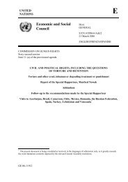
Figure 2.1: Halo of PPN NGC 7027 observed<br />
<strong>by</strong> the HST.<br />
Figure 2.2: Details of PPN NGC 7027<br />
observed <strong>by</strong> the HST.<br />
NGC 7027 is the best studied of the young PNe. The photograph in Fig. 2.1 is<br />
taken <strong>by</strong> the WFPC2 instrument on-board the HST and shows details which consist<br />
of three distinct components: (1) an ellipsoidal shell depicting the ionised core, (2) a ellipsoidal shell<br />
bipolar hourglass structure outside the ionised core represents the excited molecular bipolar hourglass<br />
structure<br />
hydrogen or photo-dissociation region and (3) a nearly spherical outer region seen<br />
in dust scattered light is the cool, neutral molecular envelope. The interface region<br />
spherical outer<br />
region<br />
between the inner shell and the bipolar hourglass is structured and filamentary, structured and<br />
filamentary<br />
suggesting the existence of hydrodynamic instabilities (Latter et al. 2000 [89]).<br />
When it has been initially at its AGB stage the ejection of the outer star layers<br />
has occurred at a low rate and has been spherical. The HST photo reveals that the<br />
initial ejection events have happened episodically to produce the concentric shells. concentric shells<br />
This evolution culminated in a vigorous ejection of all of the remaining outer layers,<br />
which produced the bright inner regions. At this later stage the ejection have been bright inner regions<br />
non-spherical, and dense clouds of dust condensed from the ejected material. Cox<br />
et al. (2002 [31]) have found a notable series of lobes and openings in the molecular lobes and openings<br />
shell. These features are point symmetric about the centre, which implies recent<br />
activity <strong>by</strong> collimated outflows with a multiple, bipolar geometry. collimated outflows<br />
Fig. 2.2 depicts a HST/NICMOS and WFPC2 composite image, accentuating the<br />
innermost region of the nebula. The central star is clearly revealed and the stellar<br />
temperature was determined to be about 198000 K. Furthermore, it was found that<br />
the photo-dissociation layer is very thin with a bi-conical shape and lies outside the<br />
ionised gas (Latter et al. 2000 [89]).
16 2. PLANETARY NEBULAE<br />
dark edge-on disc<br />
radial “searchlight<br />
beam”<br />
circular arcs<br />
faint radial streaks<br />
Cat’s Eye Nebula<br />
multiple jet-like<br />
outflows?<br />
CRL 2688 - Egg Nebula<br />
Figure 2.3: Halo of PPN CRL 2688 observed<br />
<strong>by</strong> the HST.<br />
Figure 2.4: Infrared-details of PPN<br />
CRL 2688 observed <strong>by</strong> the HST.<br />
The high resolution image from the HST/WFPC2 instrument in Fig. 2.3 shows<br />
(1) a remarkable dark edge-on disc obscuring the central star, (2) a pair of radial<br />
“searchlight beam” like features, criss-crossed <strong>by</strong> (3) a large number (at least 25) of<br />
roughly circular arcs around the center. The arcs probably represent local peaks in<br />
a quasi-periodic mass ejection process. Very faint radial streaks can be seen within<br />
the “searchlight-beam” structures implying that these are jets of matter (Sahai et<br />
al. 1995 [130]).<br />
The arcs of CRL 2688 illustrate a history of mass ejection of a red giant star for<br />
about 12700 years. They represent dense shells of matter within a smooth cloud, and<br />
show that the rate of mass ejection from the central star has varied on time scales of<br />
about 150 to 450 years throughout its mass loss history and lasting over periods of<br />
75 to 250 years. There exist two models of creating the “searchlight beams”. Either<br />
they are formed as a result of starlight escaping from ring-shaped cavities (Sahai et<br />
al. 1998 [131]). Such cavities may be carved out <strong>by</strong> a tumbling, high-velocity outflow<br />
(about 320 km s −1 ). Or alternatively, they may result from starlight reflected off<br />
fine jet-like streams of matter being ejected from the central region, and confined<br />
to the walls of a conical region around the symmetry axis (Remark: see also the<br />
appearance of jets in the Cat’s Eye Nebula in section 2.2.3 on page 25).<br />
Fig. 2.4 (Sahai et al. 1998 [128]) shows the inner structure observed with the<br />
HST/NICMOS instrument. It reveals, that the dying star ejects matter at high<br />
speeds along a preferred axis and may even have multiple jet-like outflows. The<br />
torus along the assumed stellar equator or the orbital plane of a binary object is<br />
also visible.
2.2. Examples 17<br />
HD 44179 - Red Rectangle Nebula<br />
The image presented in Fig. 2.5 has<br />
been taken with the HST/WFPC2 instrument<br />
and shows the following fea-<br />
tures: (1) X-shaped structure, (2) lin- X-shaped structure<br />
ear features, which look like the “rungs”<br />
of a ladder and (3) dark band passing dark band<br />
across the central star. The Red Rectangle<br />
Nebula is associated with a post-<br />
Figure 2.5: The PPN HD 44179 observed<br />
<strong>by</strong> the HST/WFPC2.<br />
linear features<br />
AGB binary system (Cohen et al. 2004 binary system<br />
[27]). It turned out that the star in the<br />
centre is actually a close pair of stars<br />
that orbit each other with a period of<br />
322 days, a semi-major axis of a sini =<br />
0.32 AU and an eccentricity of e = 0.34<br />
(e.g. Men’shchikov et al. 2002 [102]). Interactions between these stars have probably<br />
caused the ejection of the thick dust disc that obscures our view towards the binary.<br />
The “rungs” show a quasi-periodic spacing, suggesting that they have arisen from<br />
discrete episodes of mass loss from the central star, separated <strong>by</strong> a few hundred<br />
years. Soker (2004 [143]) has argued that the bi-conical shape of the nebula can be<br />
formed <strong>by</strong> intermittent jets generated <strong>by</strong> the accreting companion star. intermittent jets?<br />
OH231.8+4.2 - Rotten Egg Nebula<br />
Fig. 2.6 illustrates the HST/WFPC2<br />
image of the Rotten Egg Nebula, also<br />
known as the Calabash Nebula, extending<br />
1.4 light-years in diameter and located<br />
about 5000 light-years from Earth<br />
in the constellation Puppis. A Mira vari- Mira variable star<br />
able star, known as QX Pup, is embed-<br />
ded within the evolved bipolar nebula evolved bipolar<br />
nebula<br />
OH 231.8+4.2. This central star pulsates<br />
with a period of about 700 days,<br />
which is remarkable in the light of its<br />
position at the heart of such an unusual<br />
object (Kastner et al. 1999 [79]). Due to<br />
the high speed of the stellar gas accelerated<br />
<strong>by</strong> the radiative pressure, shock<br />
fronts are formed on impact and heat<br />
the surrounding gas. It is believed that<br />
Figure 2.6: The PPN OH231.8+4.2 observed<br />
<strong>by</strong> the HST/WFPC2.<br />
such interactions dominate the formation process in PNe. Much of the gas flow observed<br />
today seems to stem from a sudden acceleration that took place only about<br />
800 years ago. Approximately 1000 years from now the Calabash Nebula will become<br />
a fully developed bipolar PN (Bujarrabal et al. 2002 [20]).
18 2. PLANETARY NEBULAE<br />
filamentary<br />
structure<br />
loops and arcs<br />
dense knots<br />
enhanced bands<br />
petal-like<br />
appearance<br />
limb-brightened<br />
knotty structure<br />
2.2.2 Round and Elliptical<br />
NGC 6720 - Ring Nebula, M57<br />
Figure 2.7: Halo of the PN NGC 6720<br />
observed <strong>by</strong> the Subaru Telescope.<br />
Figure 2.8: The PN NGC 6720 observed<br />
<strong>by</strong> the HST/WFPC2.<br />
High-resolution images of the Ring Nebula taken with the Subaru Telescope<br />
(Komiyama et al. 2000 [84], see Fig. 2.7) reveal the fine structure of the inner and<br />
outer halos and other features: (1) filamentary structure of the inner halo consisting<br />
of loops and arcs, (2) small-scale structures at the main ring like dense knots and<br />
(3) enhanced bands of emission running across the central cavity. The expansion<br />
velocity of the PN of 45 km s −1 implies a expansion age of about 1500 ± 220 years<br />
(O’Dell et al. 2002 [110]).<br />
Figure 2.9: Details in the PN NGC 6720.<br />
Subimages taken from Fig. 2.8.<br />
The innermost part of the inner halo<br />
just outside of the main ring of the nebula<br />
shows a filamentary structure consisting<br />
of loops and knots, which gives a<br />
petal-like appearance to the inner halo.<br />
The outer halo is found to show a limb-<br />
brightened knotty structure similar to<br />
the inner halo, but at much fainter levels.<br />
However, the typical size of the<br />
knots is clearly different between the two<br />
halos. The corresponding lifetime, which is estimated from the size divided <strong>by</strong> the<br />
thermal velocity, is 400 years and 1200 years (see therefore Komiyama et al. 2000 [84]).<br />
The HST image of the Ring Nebula (see Fig. 2.8) displays a host of subarcsecond<br />
dark knots or globules around the periphery of the nebula (see also Fig. 2.9). The<br />
fact that no globules are seen projected against the central region demonstrates that<br />
their distribution is in fact toroidal or cylindrical, rather than spherical. Thus the
2.2. Examples 19<br />
Ring Nebula is in reality a non-spherical, axisymmetric PN (like many other PNe), non-spherical,<br />
axisymmetric<br />
which are coincidentally seen from a direction close to its axis of symmetry (Bond<br />
et al. 1998 [15]).<br />
Spectroscopic investigations show conclusively<br />
that the inner halo cannot have the<br />
form of a radially expanding, spherical shell,<br />
but rather have to be a bipolar appearance<br />
(Bryce et al. 1994 [17]). The very faint outer<br />
halo is probably the remnants of the original<br />
AGB superwind, expanding radially outward<br />
with a velocity of about 5 km s −1 .<br />
Fig. 2.10 gives an excellent view of the<br />
Ring Nebula and its extended halo in in- extended halo<br />
frared wavelength taken <strong>by</strong> the Spitzer Space<br />
Telescope (SST) and shows several looping looping structures<br />
structures in the outer halo as well as the<br />
two bright streaks crossing the central re- bright streaks<br />
gion. Additional observations <strong>by</strong> O’Dell et<br />
al. (2002 [110]) indicate that the streaks are<br />
formed <strong>by</strong> material inside of the main ring.<br />
Figure 2.10: Halo of PN NGC 6720<br />
observed <strong>by</strong> the Spitzer Space Telescope<br />
in Infrared Wavelength.
20 2. PLANETARY NEBULAE<br />
filamentary<br />
structure<br />
loops and arcs<br />
NGC 7293 - Helix Nebula<br />
Figure 2.11: Halo of PN NGC 7293<br />
observed <strong>by</strong> the Kitt Peak National<br />
Observatory and the HST/ACS.<br />
The picture shown in Fig. 2.11, is a composite<br />
of images from the ACS/WFC instrument<br />
on-board the HST combined with the<br />
wide view taken at the Kitt Peak National<br />
Observatory. It reveals a filamentary struc-<br />
ture consisting of loops and arcs in the halo<br />
and thousands of comet-like filaments, also<br />
comet-like filaments<br />
“cometary knots” known as cometary knots. The model de-<br />
twisted components<br />
radial rays<br />
multiplicity of axes<br />
knots are<br />
primordial?<br />
Figure 2.12: Details of PN NGC 7293<br />
observed <strong>by</strong> the HST. Subimage taken<br />
from Fig. 2.11.<br />
rived from the image consists of two twisted<br />
components of the main ring, radial rays<br />
surrounding the main ring and a multiplicity<br />
of axes of the outflow (see therefore O’Dell<br />
et al. 2004 [112]). The filamentary components<br />
including the cometary knots appear<br />
to be located in a planar regime as noted <strong>by</strong><br />
O’Dell 1998 [109]. Speck et al. (2002 [146])<br />
determined a lower limit of the PN shell<br />
mass of about 1.5M⊙.<br />
Fig. 2.12 displays a detailed view of the<br />
cometary knots in the Helix Nebula. Calculations<br />
of the neutral core masses of the<br />
cometary knots from the observed extinction<br />
indicate masses of about 1.5 10 −5 M⊙<br />
for the best observed knots (O’Dell & Handron<br />
1996 [111]). 313 of these objects were<br />
detected and project a total number of the<br />
entire nebula of 3500. Investigations show<br />
a lifetime exceeding that of the PN stage.<br />
Spatial motions of the knots were measured<br />
<strong>by</strong> O’Dell et al. (2002 [110]). It was found<br />
that the knots originate in or close to the<br />
main ionisation front and possibly in the<br />
neutral zone outside of this. Various physical models are advanced enough to explain<br />
the presence of such cometary knots. Rayleigh-Taylor instabilities seem to be<br />
the most likely source. However, the less likely possibility cannot be ruled out that<br />
these knots are primordial, i.e. going back to the origin formation of what is now<br />
the central star. Rayleigh-Taylor instabilities can either result from the original PN<br />
ionisation front or with stellar wind interactions with the inside of the PN.
2.2. Examples 21<br />
NGC 6853 - Dumbbell Nebula, M27<br />
Fig. 2.13 is a composite image that includes<br />
eight hours of exposure through a<br />
Hα-filter, tracing the complex details of the<br />
nebula’s faint outer halo which spans light- faint outer halo<br />
years. Features which can be located on<br />
this detailed image are (1) a halo with substructures,<br />
(2) numerous dense knots and dense knots<br />
(3) axisymmetric bands of matter in the cen- axisymmetric bands<br />
tral region. The inhomogeneous halo con-<br />
tains various structures, such as radial fila- radial filaments,<br />
ments, arcs and arc-like features (Papamastorakis<br />
et al. 1993 [114]). The bright jetlike<br />
filaments located at the nebula interior<br />
seem to obscure the ionising radiation from<br />
the central star resulting in a dimming of<br />
Figure 2.13: Halo of PN NGC 6853<br />
observed <strong>by</strong> Robert Gendler.<br />
the halo along their directions. The bow-shaped appearance of the halo is probably<br />
related to an interaction of the nebula with the ISM.<br />
arcs and arc-like<br />
features<br />
Perpendicular to the long axis of the elongated PN is a skewed, bright-rimmed bright-rimmed<br />
elliptical form<br />
elliptical form possessing several internal structures. This geometry suggests a prolate<br />
spheroid with abroad equatorial concentration of material that is viewed nearly<br />
in the plane of the equator (O’Dell et al. 2002 [110]).<br />
The close-up image of M27, displayed in<br />
Fig. 2.14, show many dense knots, but their<br />
shapes vary. Some look like fingers pointing<br />
at the central star, located just off the upper<br />
left of the image; others are isolated clouds,<br />
with or without tails. Their typical size is<br />
about 1000 AU’s in diameter and each contains<br />
as much mass as three Earths, about<br />
10 −5 M⊙ (Meaburn & Lopez 1993 [100]). The<br />
knots are forming at the interface between<br />
the hot, ionised and cool, neutral portion of<br />
Figure 2.14: Details of PN NGC 6853<br />
observed <strong>by</strong> the HST/WFPC2.<br />
the nebula. This area of temperature differentiation moves outward from the central<br />
star as the nebula evolves. In the Dumbbell Nebula we are seeing the knots soon<br />
after this hot gas passed <strong>by</strong>.<br />
Very few knots have a clear cusp and tail structure of the prototype cometary cusp/tail structure<br />
knots found in the Helix Nebula. Radial tails become more common at larger dis- Helix Nebula<br />
tances from the central star. This indicates that we are seeing intrinsically radial<br />
structures but under a variety of orientations (see O’Dell et al. 2002 [110]).
22 2. PLANETARY NEBULAE<br />
disc-like structure<br />
comet-shaped<br />
objects<br />
elliptically shaped<br />
lobes<br />
inner bright shell<br />
external circular<br />
shell<br />
NGC 2392 - Eskimo Nebula<br />
Figure 2.15: The PN NGC 2392 observed<br />
<strong>by</strong> the HST/WFPC2.<br />
Figure 2.16: Detail of PN NGC 2392 observed<br />
<strong>by</strong> the HST/WFPC2. Subimages taken from<br />
Fig. 2.15.<br />
In this HST image (see Fig. 2.15),<br />
one can see that the “parka” is really<br />
a disc-like structure (similar to the He-<br />
lix Nebula) including a ring of comet-<br />
shaped objects, with their tails streaming<br />
away from the central star. The Eskimo’s<br />
“face” also contains some fascinating<br />
details. It is composed of two<br />
elliptically shaped lobes of matter stream-<br />
ing above and below the dying star. In<br />
this photo, one bubble lies in front of<br />
the other, obscuring part of the second<br />
lobe. The inner bright shell has a pro-<br />
late structure, with the major axis oriented<br />
very closely along the line of sight,<br />
while the external circular shell has a<br />
more oblate structure (e.g. Phillips &<br />
Cuesta 1999 [118]).<br />
The lobes are not smooth but<br />
have filaments of denser matter.<br />
Each bubble is about 1 ly<br />
long and about 0.5 ly wide. The<br />
origin of the comet-shaped features<br />
in the “parka” remains uncertain<br />
(see Fig. 2.16). One possible<br />
explanation is that these<br />
filamentary objects formed <strong>by</strong> a<br />
collision of slow- and fast-moving<br />
material <strong>by</strong> Rayleigh-Taylor<br />
instabilities or <strong>by</strong> an interaction<br />
of a collimated outflow with the outer shell, which also could explain the X-ray emissions<br />
measured <strong>by</strong> the XMM spacecraft (Guerrero et al. 2005 [61]).<br />
Unlike the Helix Nebula, where the tails beyond the knots are nearly linear structures<br />
bounded <strong>by</strong> radial lines from the central star, the tails related to the Eskimo<br />
Nebula’s knots only sometimes are well bounded. They definitely lie close to radial<br />
lines, but they often deviate within the tail feature and show orientatios up to 8 ◦<br />
from the radial direction. Furthermore, many of the tails are widen faster than the<br />
shadow of the bright knot at their head (O’Dell et al. 2002 [110]).
2.2. Examples 23<br />
NGC 6369 - Little Ghost Nebula<br />
Fig. 2.17 shows an image taken from the<br />
PN NGC 6369. The HST photograph, captured<br />
with the WFPC2 instrument depicts<br />
remarkable details of the ejection process<br />
that are not visible from ground-based telescopes<br />
because of the blurring produced <strong>by</strong><br />
the Earth’s atmosphere. The prominent<br />
blue-green ring, approximately 1 ly, marks<br />
the location where the energetic UV radiation<br />
ionises the gas in the PN. Even far-<br />
ther outside the main ring of the nebula, main ring<br />
one can see fainter arcs of gas that were fainter arcs<br />
lost from the star at the beginning of the<br />
ejection process.<br />
Figure 2.17: The PN NGC 6369 observed<br />
<strong>by</strong> the HST/WFPC2.<br />
Spectroscopic observations from Monteiro et al. (2004 [104]) leads to a mass of<br />
1.8M⊙ for the ionised gas and from evolutionary models a mass of about 0.65M⊙<br />
for the central object was derived. Consequently, this implies an initial mass for the<br />
stellar AGB progenitor of ≃ 3M⊙.<br />
NGC 3132 - Eight-Burst Nebula<br />
NGC 3132 (see HST/WFPC2 image in<br />
Fig. 2.18) is nearly 0.5 ly in diameter, and<br />
at a distance of about 2000 ly it is one of<br />
the nearer known PNe. The gases are expanding<br />
away from the central star with a<br />
velocity of about 14.5 km s −1 . This image<br />
clearly shows two stars near the centre of<br />
the nebula, a bright white one, and an adjacent,<br />
fainter companion to its upper right.<br />
(A third, unrelated star lies near the edge<br />
of the nebula.) The faint partner is actually<br />
the star that has ejected the nebula. An-<br />
Figure 2.18: The PN NGC 3132 observed<br />
<strong>by</strong> the HST/WFPC2.<br />
other peculiarity of this PN are the twisted twisted dust lanes<br />
dust lanes in the front and behind the ionised central cavity.<br />
In low-resolution images NGC 3132 appears ellipsoidal, but simple shell models<br />
do not explain all of the observed characteristics. Monteiro et al. (2000 [103]) has<br />
proposed a model in which the nebula has an hourglass structure that is being viewed<br />
at 40 ◦ relative to the light of sight.
24 2. PLANETARY NEBULAE<br />
lowest mass<br />
progenitor star<br />
low total nebular<br />
mass<br />
remarkable<br />
textures<br />
circular ring<br />
long streamers<br />
irregular ring<br />
multiple shell<br />
structure<br />
IC 418 - Spirograph Nebula<br />
Figure 2.19: The PN IC 418 observed<br />
<strong>by</strong> the HST/WFPC2.<br />
Fig. 2.19 shows an image of the Spirograph<br />
Nebula (IC 418) obtained with the<br />
WFPC2 of the Hubble Space Telescope which<br />
disclose a complex morphology and the bright<br />
central star. This central star with a derived<br />
luminosity of 2850L⊙ was placed on a stellar<br />
evolutionary track (see e.g. Iben 1995 [72])<br />
among the lowest mass progenitor stars for<br />
PNe, consistent with the low total nebular<br />
masses of 0.2 to 0.7M⊙ assumed for the model<br />
proposed <strong>by</strong> Meixner et al. (1996 [101]. Furthermore,<br />
a mass loss rate of a few 10 −5 M⊙<br />
yr −1 over a period of 3000 years followed <strong>by</strong><br />
an abrupt decrease 2000 years ago when the<br />
star presumably left the AGB. The remark-<br />
able textures seen in the nebula are newly<br />
revealed <strong>by</strong> the Hubble telescope, and their origin is still uncertain.<br />
NGC 6751<br />
Figure 2.20: The PN NGC 6751 observed<br />
<strong>by</strong> the HST/WFPC2.<br />
Fig. 2.20 displays an image of the Planetary<br />
Nebula NGC 6751 obtained with the<br />
WFPC2 instrument of the Hubble Space Telescope.<br />
The nebula shows a very complex<br />
morphology. Blue regions mark the hottest<br />
gas, which forms a roughly circular ring a-<br />
round the central stellar remnant. Parts in<br />
orange and red show the locations of cooler<br />
gas. The cool gas tends to lie in long stream-<br />
ers pointing away from the central star, and<br />
in a surrounding, irregular ring at the outer<br />
edge of the nebula. The origin of these cooler<br />
clouds within the nebula is still uncertain,<br />
but the streamers are clear evidence that their<br />
shapes are affected <strong>by</strong> radiation and stellar<br />
winds from the hot star at the centre. The<br />
star’s surface temperature is estimated to be<br />
about 140000 K. Furthermore, observations have indicated the presence of a multiple<br />
shell structure in the faint envelope (Chu et al. (1991 [24]).
2.2. Examples 25<br />
2.2.3 Bipolar and Quadrupolar<br />
NGC 6543 - Cat’s Eye Nebula<br />
Figure 2.21: Halo of the PN NGC 6543<br />
observed <strong>by</strong> the NOT.<br />
Figure 2.22: The PN NGC 6543 observed<br />
<strong>by</strong> the HST/ACS.<br />
Fig. 2.21 shows the extended halo of the PN NGC 6543 observed <strong>by</strong> the Nordic<br />
Optical Telescope (NOT). Many non-radial filamentary structures are observable. non-radial<br />
A more detailed image of the nebula’s core was taken with Hubble’s Advanced<br />
Camera for Surveys (ACS) and can be seen in Fig. 2.22. It reveals eleven or even<br />
filamentary<br />
structures<br />
more concentric rings, or shells, around the Cat’s Eye Nebula. These photoionised concentric rings or<br />
shells<br />
rings are almost certainly the result of periodic spherical mass pulsations <strong>by</strong> the<br />
nucleus before the Cat’s Eye Nebula formed. A good fit is obtained if the bubbles<br />
were ejected with constant mass, thickness, and ejection velocity. The model can be<br />
used to estimate the total mass of the rings, ≈ 0.1M⊙, which lies between that of<br />
the core (≈ 0.05M⊙) and the surrounding halo (≈ 0.5M⊙). Assuming an ejection<br />
speed of 10 km s −1 the inter-pulse period is 1500 ± 300 years, the same as the<br />
expansion age of the core itself. Images taken from HST of other PNe, IC 418, IC 418, NGC 7027<br />
and Hb 5<br />
NGC 7027, and Hubble 5 (Hb 5) show similar sets of multiple concentric rings<br />
(Balick & Wilson 2000 [11]).<br />
Approximately 1,000 years ago the pattern of mass loss suddenly changed, and<br />
the Cat’s Eye Nebula started forming inside the dusty shells. It has been expanding<br />
ever since, as discernible in comparing Hubble images taken in 1994, 1997, 2000, and<br />
2002 (see therefore Balick & Hajian 2004 [8]). A summary of the bipolar structure bipolar structure of<br />
the core<br />
of the PN core can be found in Balick (2004 [6])
26 2. PLANETARY NEBULAE<br />
bright elliptical<br />
ring<br />
intersecting<br />
elliptical rings<br />
arc-like structures<br />
high speed knots<br />
high surface<br />
brightness<br />
dark lanes<br />
high-velocity<br />
outflow<br />
MyCn 18 - Hourglass Nebula<br />
In the HST/WFPC2 image (Fig. 2.23)<br />
of the young PN MyCn 18 a bright ellipti-<br />
cal ring can be seen. The hot central star<br />
within this ring is shown clearly off-centre.<br />
Several other features has been also revealed<br />
which are completely new and unexpected.<br />
For example, there is a pair of intersecting<br />
elliptical rings in the central region which<br />
appear to be the rims of a smaller hourglass<br />
(Sahai et al. 1995 [130]). The arc-like struc-<br />
tures on the hourglass walls could be (1) the<br />
remnants of discrete shells ejected from the<br />
star when it has been younger (e.g. as seen<br />
in the Egg Nebula), (2) flow instabilities, or<br />
Figure 2.23: The PN MyCn 18 ob-<br />
(3) the result from the action of a narrow<br />
served <strong>by</strong> the HST/WFPC2.<br />
beam of matter intersecting the walls. Furthermore,<br />
high speed knots with outflow velocities up to about 630 km s−1 are<br />
located apparently along the main axis of the bipolar shape. Spectrometric observations<br />
also indicate that some pairs of knots have been ejected in opposing directions<br />
with the same velocity. Among several possible explanations of these hypersonic<br />
knots O’Connor et al. (2000 [108]) preferred the model of a recurrent nova-like ejection<br />
from a central binary star.<br />
IC 4406 - Retina Nebula<br />
Figure 2.24: The PN IC 4406 observed<br />
<strong>by</strong> the HST/WFPC2.<br />
hancement surrounding the central object.<br />
An image of the seemingly square nebula<br />
IC 4406 can be seen in Fig. 2.24. Like<br />
many other PNe, it exhibits a high degree<br />
of symmetry. The central star is faint and<br />
seen against the high surface brightness neb-<br />
ula. One of the most interesting features<br />
of IC 4406 is the irregular lattice of dark<br />
lanes that criss-cross the centre of the nebula.<br />
These lanes are about 160 AU wide<br />
(see O’Dell et al. 2002 [110]). Data from observations<br />
done <strong>by</strong> Sahai et al. (1991 [132])<br />
has revealed the presence of a high-velocity<br />
outflow directed along the major axis of the<br />
bipolar shape. It seems that the outflow has<br />
been collimated <strong>by</strong> an toroidal density en
2.2. Examples 27<br />
NGC 6302 - Bug or Butterfly Nebula<br />
Figure 2.25: The PN NGC 6302 observed<br />
<strong>by</strong> Wendel and Flach-Wilken.<br />
Figure 2.26: Details of the PN NGC 6302<br />
observed <strong>by</strong> the HST/WFPC2.<br />
The surrounding of the PN NGC 6302 shows Fig. 2.25 whereas Fig. 2.26 depicts<br />
a more detailed image captured <strong>by</strong> the HST/WFPC2 instrument. NGC 6302 is<br />
known as the prototypical “butterfly” PN, with the fast wind of the hot central star<br />
channelised into a bipolar shape <strong>by</strong> a central dense structure.<br />
This butterfly-shaped PN is also known as one of the brightest and most extreme<br />
PNe. A dense equatorial lane, probably a dusty disc obscuring the central star, can dense equatorial<br />
lane<br />
be observed surrounding the central object. From spectral measurements a mass of<br />
at least 0.03M⊙ was derived for this dust disc (Matsuura et al. 2005 [98]). Some<br />
other models suggest a much more disc mass. The innermost region of this massive<br />
disc shows an ionised shell which was produced <strong>by</strong> the very hot central star. This ionised shell<br />
star is believed to be one of the hottest PN central star known with an temperature<br />
of 380000 K (Pottasch et al. 1996 [119]).<br />
Furthermore, the bipolar axis shows a distinct change with distance from the distinct change of<br />
bipolar axis<br />
central object. Also the central dust lane looks slightly deformed. Several of such<br />
observed structures are similar to those predicted in the warped-disc model of Icke<br />
(2003 [76]).
28 2. PLANETARY NEBULAE<br />
dense ionised core<br />
spherical, bipolar<br />
lobes<br />
filamentary bipolar<br />
nebula<br />
hypersonic velocity<br />
features<br />
inner and outer<br />
lobes<br />
ansae<br />
dense disc<br />
close pair of stars<br />
Mz 3 - Ant Nebula<br />
Figure 2.27: The PN Mz 3 observed <strong>by</strong><br />
the HST/WFPC2.<br />
Fig. 2.27 displays a detailed view of the<br />
complex structure of the young bipolar nebula<br />
Mz 3 or Ant Nebula. This image was<br />
combined <strong>by</strong> pictures of two observations<br />
with the HST/WFPC2 instrument using<br />
slightly different filters. Detailed investigations<br />
of the bipolar PN Mz 3 reveals a dense<br />
ionised core with almost spherical, bipolar<br />
lobes. These are contained within a much<br />
more extensive filamentary bipolar nebula.<br />
The expansion velocity of the inner lobes is<br />
measured to be about 50 km s −1 whereas<br />
the walls of the outer bipolar structure expand with about 90 km s−1 . A pair of<br />
hypersonic velocity features along the bipolar axis of the nebula reaches velocities<br />
of ≃ 500 km s−1 (Redman et al. 2000 [121]).<br />
M2-9<br />
Figure 2.28: The PN M2-9 observed <strong>by</strong><br />
the HST/WFPC2.<br />
The HST/WFPC2 image of the bipolar<br />
PN M2-9 shown in Fig. 2.28 depicts several<br />
details like inner and outer lobes of the<br />
bipolar regions on both sides of the centre,<br />
ansae at the main axis of the nebula and<br />
a dense disc obscuring the central region.<br />
The central star in M2-9 is known to be<br />
one of a very close pair of stars. A model<br />
proposed <strong>by</strong> Livio & Soker (2001 [92]) assuming<br />
that the system consist of an AGB<br />
star or post-AGB star and a White Dwarf<br />
companion with an orbital period of about 120 years. It is even possible that the<br />
stars are engulfed in a common envelope of gas. Another explanation could be that<br />
the gravity of the compact White Dwarf rips weakly bound gas of the AGB star<br />
generating a thin and dense disc.
2.3. Global Models to Shape a PN 29<br />
2.3 Global Models to Shape a PN<br />
The observed morphologies of PNe range from round to elliptical to bipolar to pointsymmetric,<br />
whereas their progenitors, the AGB stars, show spherical symmetry in<br />
their envelopes (e.g. Lucas et al. 1992 [93] Sahai & Bieging 1993 [127], Neri et<br />
al. 1998 [106]). Therefore, it is certain that the interacting-winds process plays a<br />
role in the shaping of the nebula.<br />
2.3.1 Multiple-<strong>Winds</strong> Model<br />
In general main categories of PN shapes like round, elliptical, bipolar, point-symmetric<br />
and irregular can be observed. To explain such various shapes detailed theoretical<br />
and observational efforts have to be undertaken to combine all essential physical<br />
effects and all possible scenarios together to a complete theory which can interpret<br />
the phenomenon of a PN.<br />
First approaches were made when Kwok et al. (1978 [88]) formulated the inter- interacting wind<br />
theory<br />
acting winds theory (or two wind model), in which the slow wind from the AGB<br />
expansion is swept up <strong>by</strong> a later-developed fast wind originating from the central<br />
star and forming the dense PN shell. Then it has been studied in more detail<br />
<strong>by</strong> Kwok (1982 [85]) and a quantitative model has been constructed <strong>by</strong> Kahn &<br />
West (1985 [78]).<br />
Furthermore, a refined model is needed for point-symmetric and irregular shaped<br />
PNe. Also the observed small-scale-structures like features in the halos, jets, ansae<br />
and knots demand a theoretical model. We also have to take the three-dimensional perspective<br />
structure and the different perspectives into account, i.e. some bipolar nebula appear<br />
elliptical or even round when their major axis is oriented fairly close along the line<br />
of sight.<br />
The multiple-winds model can describe the global shaping of a PN but fail to<br />
explain many small-scale structures. It is possible to modify and refine this model<br />
to get further interesting results. E.g. if we rewrite the boundary conditions of the<br />
multiple-winds problem we obtain new classes of shapes.<br />
2.3.2 Aspherical <strong>Mass</strong> <strong>Loss</strong> of AGB stars<br />
In the ideal case of the multiple-winds model a spherical fast wind from the central<br />
star of a PN or later the White Dwarf blows into the also spherical slow and much<br />
denser wind of the progenitor AGB star. The result is an exact spherical shaped PN.<br />
However, if the slow wind of the AGB star is generated <strong>by</strong> aspherical mass loss then<br />
an aspherically shaped PN will be formed. Now we have to think about a model<br />
which can explain such aspherical mass losses.<br />
One explanation is stellar rotation which generates an asphericity of the luminos- stellar rotation<br />
ity or alternatively effective temperature at the stellar photosphere (see e.g. Dorfi<br />
& Höfner 1996 [39]). Due to the strong dependence of the dust formation process<br />
on the temperature and density these small deviations from spherical symmetry will<br />
affect the condensation of dust and therefore the mass loss rate. The result is a<br />
preferred mass loss in the equatorial plane and the formation of a pole-to-equator
30 2. PLANETARY NEBULAE<br />
stellar companion<br />
nonaxisymmetric<br />
structure<br />
dynamos in<br />
AGB stars<br />
magnetic shaping<br />
binary and<br />
stellar disc<br />
magnetic fields<br />
in central stars<br />
stellar spots<br />
density distribution in the vicinity of the AGB star. When the fast wind from the<br />
central object succeeding the AGB phase sweeps into this aspherical density distribution<br />
it is possible to form elliptical up to less-developed bipolar PNe as shown<br />
e.g. in Reimers (1999 [122]) and Reimers et al. (2000 [123]).<br />
Another model is based on the existence of a stellar companion, where the de-<br />
parture from axisymmetric AGB wind structure can also form elliptical to bipolar<br />
PNe (Livio 1982 [91]). Furthermore, close binaries can produce an accretion disc<br />
and jets, which induces a collimated fast wind. This is leading to nonaxisymmetric<br />
structures and very pronounced bipolar shapes. Soker & Rappaport (2001 [145])<br />
looked into this problem and described the mechanism to form asymmetric PNe <strong>by</strong><br />
the variation of the mass loss, i.e. the preferred mass loss in the orbital plane and/or<br />
the occurrence of a jet-like outflow formed at the accretion disc of the companion<br />
star.<br />
2.3.3 The Role of Magnetic Fields<br />
Dynamos in AGB stars can be the origin of magnetic fields. If this field is strong<br />
enough to interact with the matter and shows a more regular structure, then it is<br />
possible to get bipolar outflows like jets or influence the stellar surface quantities<br />
(like temperature or pressure). These processes are able to shape aspherical PNe.<br />
Magnetic fields in the stellar vicinity<br />
Blackman et al. (2001 [13]) investigated the shaping of PNe <strong>by</strong> magnetic fields<br />
originated from dynamos in AGB stars. They predict that magnetic fields should be<br />
apparent in the winds of AGB stars and Proto-PNe and also that collimated flows<br />
in Proto-PNe should have signatures of ordered magnetic fields. The dynamo model<br />
is based on a rapid rotation of the AGB core.<br />
If in a close binary system the magnetic field is coupled to the surrounding disc<br />
it is possible to get a powerful MHD wind that might help to explain multishell or<br />
multipolar PNe (Blackman et al. 2001 [14]). The precession of the disc can change<br />
the symmetry axis and therefore form the observed multipolar PN-shapes.<br />
Magnetic fields on stellar surfaces<br />
Nowadays magnetic fields are detected in central stars of PNe (see Jordan et<br />
al. 2005 [77]) and in White Dwarfs. The magnetic fields observed in White Dwarfs<br />
can be explained as relics from magnetic fields in the main-sequence progenitors<br />
which are enhanced <strong>by</strong> magnetic flux conservation during the contraction of the<br />
core. The discovery of magnetic fields in White Dwarfs (e.g. Aznar Cuadrado et<br />
al. 2004 [3]) indicates that a substantial fraction of White Dwarfs have a weak<br />
magnetic field.<br />
Also proposed is the influence of the occurrence of cool stellar spots on the mass<br />
loss rate of the AGB star (Soker 2000 [141]). A stellar magnetic field could produce<br />
such cool spots <strong>by</strong> a non-linear magnetic dynamo like that in the numerical SHD<br />
simulations presented <strong>by</strong> Dorch (2004 [35]). The idea to produce an aspherical mass<br />
loss <strong>by</strong> an inhomogeneous temperature distribution at the the stellar surface will be<br />
picked up in this thesis. The used model is described in detail in Section 4.3.
2.3. Global Models to Shape a PN 31<br />
2.3.4 Interaction with the ISM<br />
Some central stars of PNe are displaced clearly from the center of the nebula. In displacement of<br />
central star<br />
many cases this indicates an interaction of the nebula with the ISM. The expanding<br />
shell of those highly evolved PNe realise the existence of the gas pressure between<br />
the stars. The material of the shells are incorporated into the ISM, thus the central<br />
star migrate out of the geometrical centre according to the stellar proper motion<br />
(see therefore e.g. Villaver et al. 2000 [152] and Kerber et al. 2004 [81]).<br />
Furthermore, the interaction affects also the shape of the PNe which gets more<br />
and more irregular due to inhomogeneities and turbulences in the ISM. This phase irregular shape<br />
is hardly be observed because as a result of the declining rate of ionised radiation<br />
from the central star such evolved PNe are rapidly dimming objects.<br />
2.3.5 MHD Models<br />
García-Segura et al. (1999 [51]) studied the influence of several effects on the formation<br />
of PNe <strong>by</strong> applying two-dimensional magneto-hydrodynamic (MHD) simulations<br />
of the interaction of two suceeding, time-independent stellar winds. The<br />
rotation of a single AGB-star can lead to an equatorially confined wind resulting in<br />
a typical hourglass shape. Further on, the combination of such a rotating AGB wind<br />
with a magnetic post-AGB wind generates highly collimated bipolar nebulae. For<br />
sufficiently strong magnetic fields ansae and jets are formed in the polar regions of<br />
the nebula. Photo-ionisation can also reproduce irregularities in the shape of simulated<br />
nebulae through instabilities in the ionisation-shock front. In special cases<br />
also cometary knots are formed.<br />
The formation of point-symmetric structures in elliptical and bipolar PNe are<br />
investigated <strong>by</strong> García-Segura (1997 [50]) and García-Segura and López (2000 [52])<br />
<strong>by</strong> using 3D MHD simulations. Therefore, these small-scale structures can be described<br />
according to a misalignment of the magnetic collimation axis with respect<br />
to the symmetry axis of the bipolar wind outflow. Distinct jets or ansae-like structures<br />
are evolving from this model depending on the mass loss rate of the collimated<br />
outflow.
32 2. PLANETARY NEBULAE<br />
AGB wind<br />
2.4 Details in PNe<br />
With high-resolution imaging a lot of detailed structures can be found in or beyond<br />
PNe. Some of these common features are described in the following subsections.<br />
2.4.1 Halo<br />
An interesting field of research are halos of PNe originating from the AGB wind<br />
before the PN forms. In the halo we can see the mass loss history of the AGB star.<br />
This is important to understand the kinematics and dynamics of the mass loss in<br />
the latest AGB phase. To study the structure of these halos can provide us with<br />
informations about the<br />
• time-dependency of mass loss,<br />
• inhomogeneity of mass loss and<br />
• interaction process of AGB winds with the ISM.<br />
A comprehensive observational study of halos around PNe has been undertaken<br />
<strong>by</strong> Corradi et al. (2003 [30]) which divides the halos into the following groups:<br />
• circular or slightly elliptical AGB halos, which contain the signature of the<br />
last thermal pulse on the AGB;<br />
• highly asymmetrical AGB halos;<br />
• candidate recombination halos, i.e. limb-brightened extended shells that are<br />
expected to be produced <strong>by</strong> recombination during the late post-AGB evolution,<br />
when the luminosity of the central star drops rapidly <strong>by</strong> a significant factor;<br />
• uncertain cases which deserve further study for a reliable classification;<br />
• non-detections.<br />
Many PNe with faint extended halos have been newly discovered as well as very<br />
expanded ones, e.g. the detection of a giant halo around the PPN NGC 7027 (Navarro<br />
et al. 2002 [105]).<br />
Multiple shells<br />
Several explanations have been proposed to describe multiple shells around PNe<br />
including cycles of magnetic activity somewhat similar to our Sun’s sunspot cycle,<br />
the action of companion stars orbiting around the dying star, and stellar pulsations.<br />
Another possibility is that the material is ejected smoothly from the star, and the<br />
rings are created later on due to formation of waves in the outflowing material. It<br />
will take further observations and more theoretical studies to decide between these<br />
and other possible explanations.
2.4. Details in PNe 33<br />
”FLIERs” (fast low-ionisation emission regions)<br />
FLIERs seem to be most common in elliptical PNe. They are supersonic outflows<br />
on opposite sides in the major axis and at the same distance from the central star<br />
(cf. ansae below). An extensive research about FLIERs and other micro-structures<br />
in PNe has been summarised in a set of four papers <strong>by</strong> Balick et al. (1993 [10],<br />
1994 [9], 1998 [7]) and Hajian et al. (1997 [64]).<br />
Rings and Arcs<br />
The bright aspherical nebulae are often found to be surrounded <strong>by</strong> faint, roughly<br />
round halos, which are signatures of the progenitor AGB envelopes produced <strong>by</strong><br />
an isotropic mass loss. A number of these halos include numerous concentric arcs,<br />
an evidence for quasi-periodic modulation of the mass loss on time scales of a few<br />
hundred years (see e.g. Hrivnak et al. 2001 [70] and Corradi et al. 2004 [29]).<br />
2.4.2 Jets, Lobes and Ansae<br />
Observations of the PPN NGC 7027 show a remarkable series of holes or cavities in<br />
the molecular hydrogen region. These features are ordered point symmetric about<br />
the central star. The most direct interpretation of these point symmetric holes is<br />
the action of multiple, bipolar outflows or jets from the central star. These are seen<br />
to be increasingly common in PNe, and well studied examples of multiple outflows<br />
showing interactions with the surrounding molecular envelope (CRL 2688 and M1- M1-16<br />
16). In both cases the jets are more prominent than in NGC 7027, but the similarity<br />
is striking (cf. Cox et al. 2002 [31]).<br />
PNe with low excitation characteristics show highly aspherical morphology illustrated<br />
in the existence of multipolar bubbles. In some objects bipolar ansae multipolar bubbles<br />
or collimated radial structures are seen indicating the presence of jets. Sahai and<br />
Trauger (1998 [129]) proposed that the shaping of those PNe is done <strong>by</strong> high-speed<br />
collimated outflows or jets during the late AGB phase and/or early Post-AGB evolutionary<br />
phase. Three pairs of low-ionisation features, called caps, ansae, and jets,<br />
are detected at or beyond the perimeter of the core of the Cat’s Eye Nebula. The<br />
two thin, radial jets do not lie along the symmetry axis of any other features. Long<br />
term observations are made but no evidence of a lateral change has been seen (Balick<br />
2004 [6] and Balick & Haijan 2004 [8]). One prototype of a PN with ansae is the<br />
Saturn Nebula, NGC 7009. Sabbadin et al. (2004 [126]) analysed the 3D-structure NGC 7009<br />
‘Saturn Nebula’<br />
and several parameters of the nebula and the central star. The ansae expand with<br />
a velocity larger than the rest of the nebula. The ansae material is ejected with<br />
a higher velocity in the PPN phase. The proper motion of the ansae has been<br />
measured <strong>by</strong> Fernández et al. (2004 [43]) giving a velocity of 114 ± 32 km s −1 and<br />
a dynamic age of about 910 ± 260 years. The age of the PN is determined to be<br />
around 2000 years where the ionisation of the main shell is initiated.<br />
2.4.3 Knots<br />
Dense knots of gas and dust seem to be a natural part of the evolution of PNe.<br />
They form at early stages and their shape changes as the nebula expands. Similar
34 2. PLANETARY NEBULAE<br />
cometary knots<br />
NGC 3918, K1-2<br />
and Wr 17-1<br />
knots have been discovered in other near<strong>by</strong> PNe that are all part of the same evolutionary<br />
scheme. High-resolution images taken <strong>by</strong> the HST display several knots<br />
e.g. in the Ring Nebula, the Eskimo Nebula and the Retina Nebula. The appear-<br />
ance of these knots ranges from cloudy as in the Dumbbell Nebula to cometary or<br />
finger like e.g. in the Ring, Helix and Eskimo Nebula. The most serious criticism<br />
of the cometary knots as primordial knots has been annotated <strong>by</strong> O’Dell & Handron<br />
(1996 [111]). It is therefore not possible to decide if cometary knots exist as<br />
primordial knots. Due to the extreme conditions at the late stage of the AGB star<br />
evolution gravitationally bound objects could be undetectable until they are revealed<br />
at large distances. Some issues about cometary knots (sometimes called globules)<br />
are discussed in the following papers:<br />
- Capriotti (1973 [21]): Structure and evolution of planetary nebulae (Rayleigh-<br />
Taylor instabilities, e.g. Helix Nebula, NGC 7293)<br />
- Henry et al. (1999 [66]): Morphology and composition of the Helix Nebula<br />
- Corradi et al. (1999 [28]): Jets, knots and tails in planetary nebulae (NGC 3918,<br />
K1-2, and Wr 17-1)<br />
- O’Dell et al. (2002 [110]): Knots in near<strong>by</strong> planetary nebulae (filaments in<br />
IC 4406, the Retina Nebula, as possible globule precursors)<br />
- Huggins & Mauron (2002 [71]): Small scale structure in circumstellar envelopes<br />
and the origin of globules in planetary nebulae
Part II<br />
Theoretical Models<br />
35
Chapter 3<br />
Radiation Hydrodynamics<br />
Simulation<br />
To describe a stellar interior and atmosphere we need at first a physical system<br />
which characterises the behaviour of the gas and dust embedded in a radiative<br />
environment. Since the star is in the thermodynamic equilibrium, i.e. the produced<br />
energy is equal to the radiated energy, a certain temperature and luminosity adjusts<br />
itself at the photosphere of the star. Furthermore, the physical conditions depend<br />
on the equation of state and the optical properties of the gas and dust component.<br />
The radiative energy at the photosphere is used to force dynamical processes in the<br />
stellar atmosphere which includes shock waves propagating through the atmosphere<br />
as well as the generation and destruction of molecules and dust grains.<br />
In this chapter the derivation of the used physical system, the boundary conditions<br />
and the generation of initial models are given in the special case of spherical<br />
symmetry.<br />
3.1 Basic Equations<br />
3.1.1 Conservation form<br />
The conservation form of physical equations describes the changes of a physical parameter<br />
φ (e.g. momentum, density, etc.) only due to fluxes through the boundaries<br />
and is conserved otherwise. Thus a certain measurable property of an isolated physical<br />
system does not vary as the system evolves. Therefore, the total derivative of a<br />
physical parameter integrated over the volume dV can be written as<br />
�<br />
d<br />
φdV =<br />
dt<br />
�<br />
Qi − �<br />
Sj<br />
(3.1)<br />
V (t)<br />
where Qi represents the source terms and Sj the sink terms. Because the boundaries<br />
depend on the time t we can apply Leibniz’ rule for the r.h.s.<br />
�<br />
d<br />
dt<br />
φdV =<br />
� �<br />
∂φ<br />
dV +<br />
∂t<br />
φ �u d � A . (3.2)<br />
V (t)<br />
V (t0)<br />
i<br />
37<br />
j<br />
A(t0)
38 3. RADIATION HYDRODYNAMICS SIMULATION<br />
To rewrite this equation in a compact form we use Gauß’ law<br />
�<br />
d<br />
dt<br />
V (t)<br />
φdV =<br />
�<br />
V (t0)<br />
�<br />
∂φ<br />
∂t + � �<br />
∇ · (φ �u) dV . (3.3)<br />
Another notation can be derived <strong>by</strong> using the substantial derivation ( D<br />
Dt := ∂t+�u· � ∇)<br />
�<br />
d<br />
dt<br />
V (t)<br />
φdV =<br />
�<br />
V (t0)<br />
�<br />
Dφ<br />
Dt + φ � �<br />
∇ · �u dV . (3.4)<br />
For a moving coordinate system the conservation equations take the form<br />
� �<br />
∂<br />
X dV + X u<br />
∂t V (t) ∂V (t)<br />
rel �<br />
dA = S dV , (3.5)<br />
V (t)<br />
where X is the physical quantity, S represents the source and sink terms and u rel is<br />
the relative velocity between the co-moving frame and the numerical grid. Thus, for<br />
an Eulerian grid we have u rel = u (u is the gas velocity) and for a Lagrangean grid<br />
u rel = 0. In case of an adaptive grid and spherical symmetry the relative velocity is<br />
given <strong>by</strong><br />
u rel = u − u grid , (3.6)<br />
where ugrid is the velocity component of the moving coordinate system in an inertial<br />
frame of reference<br />
u grid = ∂r<br />
. (3.7)<br />
∂t<br />
3.1.2 Gas Component<br />
Equation of Continuity<br />
This equation describes the conservation of mass within a volume V<br />
dm<br />
dt<br />
= 0 . (3.8)<br />
The physical parameter φ is the density ρ and there are no source and sink terms<br />
to include<br />
�<br />
d<br />
dt<br />
ρdV = 0 . (3.9)<br />
Thus we can write the conservation form of the continuity equation as<br />
V (t)<br />
∂<br />
∂t ρ + � ∇ · (ρ�u) = 0 . (3.10)
3.1. Basic Equations 39<br />
Energy Equation<br />
This equation describes the conservation of the energy<br />
dE<br />
dt<br />
= �<br />
i<br />
E (t)<br />
i . (3.11)<br />
The physical parameter φ is the density multiplied <strong>by</strong> the internal energy per mass<br />
ρe. But first we look at the total energy balance which includes the internal and<br />
mechanical energy<br />
∂<br />
∂t<br />
�<br />
ρ<br />
�<br />
e + 1<br />
2 v2<br />
��<br />
+ � ∇ ·<br />
� �<br />
ρ�u e + 1<br />
2 v2<br />
��<br />
= −� ∇ · �q + � ∇ · T · �u + ρ �u · � F . (3.12)<br />
If we multiply the momentum equation <strong>by</strong> �u from the left side we get the mechanical<br />
energy balance<br />
�<br />
∂<br />
ρ<br />
∂t<br />
v2<br />
�<br />
+<br />
2<br />
� �<br />
∇ · ρ�u v2<br />
�<br />
= −�u ·<br />
2<br />
� ∇P + �u · ( � ∇ · τ) + ρ �u · � F . (3.13)<br />
Now we combine these two relations and derive<br />
where<br />
∂<br />
∂t (ρe) + �∇ · (ρe�u) = −P �∇ · �u + τ : �∇�u − �∇ · �q , (3.14)<br />
τ : � ∇�u = �<br />
i,j<br />
τijui;j<br />
denotes the contraction of the viscous stress with the divergence of �u.<br />
Momentum Equation (Equation of Motion)<br />
This equation describes the conservation of the momentum<br />
d � I<br />
dt<br />
(3.15)<br />
�<br />
= �Fi . (3.16)<br />
The physical parameter φ is the density multiplied <strong>by</strong> the gas velocity ρ�u.<br />
d � I<br />
dt<br />
i<br />
�<br />
d<br />
=<br />
dt<br />
V (t)<br />
First we will start with the following approach<br />
�Ftot = ρ D�u<br />
Dt = � ∇T + ρ �<br />
(ρ�u)dV (3.17)<br />
i<br />
�fi , (3.18)<br />
where T = −PI + τ is the stress tensor which describes the momentum of the<br />
molecular processes (e.g. pressure), P is the thermodynamical pressure, τ is the
40 3. RADIATION HYDRODYNAMICS SIMULATION<br />
viscous stress and � fi are external forces. With the help of the continuity equation<br />
we get the conservation form of the equation of motion<br />
or<br />
3.1.3 Radiation Field<br />
∂<br />
∂t (ρ�u) + � ∇ · (ρ�u�u T ) = � ∇T + ρ �<br />
∂<br />
∂t (ρ�u) + � ∇ · (ρ�u�u T ) = −� ∇P + � ∇τ + ρ �<br />
i<br />
i<br />
�fi<br />
(3.19)<br />
�fi . (3.20)<br />
The radiation transfer is treated in the grey (i.e. frequency integrated) approximation.<br />
The radiation field can be characterised <strong>by</strong> moments of the specific intensity<br />
Iν defined <strong>by</strong><br />
E = 1<br />
c<br />
�∞�<br />
0<br />
∞<br />
��<br />
�F =<br />
0<br />
P = 1<br />
c<br />
�∞�<br />
0<br />
IνdΩdν = 4π<br />
J ... radiation energy density (3.21)<br />
c<br />
Iν�ndΩdν = 4π � H ... radiation energy flux (3.22)<br />
Iν�n�ndΩdν = 4π<br />
K ... radiation pressure (3.23)<br />
c<br />
The starting point of the equations needed is the radiation transfer equation (hereafter<br />
RTE), which describes the propagation of photons through a medium with the<br />
ability of absorption and emission of radiation.<br />
Special cases can be deduced from plane-parallel or spherical geometry. But we<br />
will derive the zeroth and first moment equations of the RTE in general geometry<br />
and for a moving medium. The detailed way of deduction is given in Appendix C<br />
(Radiation Transfer). Here we will only write down the moments as derived from<br />
Buchler 1983 [18] (see also Buchler 1986 [19]).<br />
Zeroth Moment Equation of the RTE<br />
ρ d<br />
dt<br />
� �<br />
E<br />
+<br />
ρ<br />
1<br />
c2 d<br />
�<br />
�u ·<br />
dt<br />
� �<br />
F + � ∇ · � F + P : � ∇�u + 1<br />
c2 �<br />
�a · � �<br />
F =<br />
�∞<br />
0<br />
q0(ω)dω (3.24)
3.1. Basic Equations 41<br />
First Moment Equation of the RTE<br />
ρ<br />
c<br />
� �<br />
d �F<br />
dt ρ<br />
3.1.4 Dust<br />
+ 1<br />
c<br />
d<br />
dt<br />
� �<br />
(�u · P) + c �∇ · P + 1 1<br />
� �<br />
(�aE) + �F · ∇�u � =<br />
c c<br />
�∞<br />
0<br />
�q(ω)dω (3.25)<br />
After the inclusion of gas and radiation we will add dust as third component in the<br />
RHD code. The process of dust formation for a carbon-rich chemistry is described<br />
as a two step process according to Sedlmayr 1989 [139]. The first step describes the<br />
condensation of supercritical nuclei out of the gas phase and the second step depicts<br />
the growth of macroscopic grains.<br />
Net Transition and Growth Rate<br />
The condensation of supercritical nuclei is determined with the net transition rate<br />
for spherical dust particles (i.e. d = 3)<br />
J = N d−1<br />
d<br />
ℓ<br />
f(Nℓ,t) 1<br />
τ<br />
, (3.26)<br />
where Nℓ is the lower limit of the dust grain sizes which may be regarded as macroscopic<br />
in the thermodynamical sense, f(Nℓ,t) denotes the number density of grains<br />
of size Nℓ and 1<br />
τ describes the net growth rate which is calculated in the case of<br />
chemical equilibrium (for more details see Appendix D). However, in general the<br />
number density f(N,t) is not known and J has to be calculated in a different way.<br />
If the thermodynamical conditions allow dust grain formation the transition rate<br />
is assumed to be equal to the nucleation rate J∗, i.e. the rate at which stable (supercritical)<br />
dust clusters are formed out of the gas phase. The implementation of<br />
the nucleation rate can also be found in Appendix D and is based on the classical<br />
nucleation theory (see Feder et al. 1966 [42]).<br />
Moment Equations<br />
The net change of the number density of dust grains containing N monomers is given<br />
<strong>by</strong> the master equation<br />
df(N,t)<br />
dt<br />
= R↑(N) − R ↑ (N) − R↓(N) + R ↓ (N) , (3.27)<br />
where the terms R↑(N) and R ↓ (N) refer to the addition of i-mers while R ↑ (N) and<br />
R↓(N) accounts for the subtraction of i-mers. To describe the dust component we do<br />
not need to handle the complex system like the master equation because fortunately<br />
the information required for a self-consistent model is contained in a few moments<br />
Kj =<br />
∞�<br />
N j/d f(N,t) . (3.28)<br />
N=Nℓ
42 3. RADIATION HYDRODYNAMICS SIMULATION<br />
adaptive grid<br />
The following set of moment equations can be derived from the master equation<br />
dK0<br />
= J<br />
dt<br />
(3.29)<br />
dKj j 1<br />
=<br />
dt d τ Kj−1 + N j/d<br />
ℓ J (1 ≤ j ≤ d) (3.30)<br />
which describe the formation, growth and evaporation of macroscopic dust grains<br />
(Gauger et al. 1990 [53]) in a comoving frame.<br />
Number Density of Free C-atoms<br />
Additionaly, we need also an equation which describes the number density of all free<br />
C-atoms in the gas phase (excluding the molecule CO) which are able to build up<br />
dust particles. Hence, we can write<br />
∂<br />
∂t nc + ∇ · (nc u) = 1<br />
τ K2 + Nℓ J (1 ≤ j ≤ d) (3.31)<br />
for the amount of condensable material.<br />
3.2 Additional Equations and Constitutive Relations<br />
3.2.1 Grid Equation<br />
The spatial distribution of the grid points is determined <strong>by</strong> the so-called grid equation<br />
developed <strong>by</strong> Dorfi & Drury (1987 [36]) which is solved together with the RHD<br />
equations. Therefore, an adaptive grid ensures proper resolution of various features<br />
like shock fronts or steep gradients. The grid equation takes the following form<br />
ˆnl−1<br />
Rl−1<br />
= ˆnl<br />
Rl<br />
, (3.32)<br />
where Rl denotes the desired resolution and nl the point concentration (for more<br />
details see Dorfi & Drury 1987 [36]).<br />
3.2.2 <strong>Mass</strong> Equation<br />
This equation describes the mass integrated up to a radius r, i.e.<br />
m(r) =<br />
�V<br />
0<br />
ρ(r)dV ′ . (3.33)
3.2. Additional Equations and Constitutive Relations 43<br />
In general the density ρ is a combination of the gas density and the dust density,<br />
but the dust density can be neglected in case of the small amount of condensable<br />
material compared to the amount of hydrogen and helium in the gas phase.<br />
3.2.3 Poisson Equation<br />
The Poisson equation describes the dependence of the gravitational potential ψ on<br />
the density distribution ρ, i.e.<br />
∆ψ = 4π Gρ . (3.34)<br />
To get the gravitational acceleration we need to solve following equation<br />
�g = − � ∇ψ (3.35)<br />
and is implemented in Eq. (3.20) as an additional external force, namely the gravitational<br />
force for a point mass<br />
�g = − GM<br />
r 2<br />
3.2.4 Equation of State (EOS)<br />
�r<br />
r = � fg . (3.36)<br />
The EOS is needed to get relations between the density and temperature of the<br />
material on the one hand and its pressure and internal energy, specific heats, etc.,<br />
on the other hand. Due to the low gas density in stellar atmospheres the ideal gas<br />
approach is a good approximation. ideal gas<br />
The following set of equations describe the relations approximated <strong>by</strong> an ideal<br />
gas:<br />
or<br />
P(ρ,e) = R<br />
µ cV<br />
T(ρ,e) = e<br />
cV<br />
ρ e pressure (3.37)<br />
temperature (3.38)<br />
ρ(P,T) = µ P<br />
R T<br />
density (3.39)<br />
e(P,T) = cV T energy (3.40)<br />
With the specific heat at a constant volume as<br />
� �<br />
∂e<br />
cV := =<br />
∂T<br />
R<br />
� �<br />
1<br />
µ γ − 1<br />
we can also write for the pressure in Eq. (3.37)<br />
V<br />
(3.41)<br />
P(ρ,e) = (γ − 1) ρ e . (3.42)<br />
Other useful quantities as the adiabatic temperature gradient<br />
� �<br />
∂lnT<br />
∇ad := =<br />
∂lnP<br />
γ − 1<br />
, (3.43)<br />
γ<br />
S
44 3. RADIATION HYDRODYNAMICS SIMULATION<br />
Mie approximation<br />
extinction efficiency<br />
the specific heat at constant pressure<br />
and the relation<br />
δ := −<br />
cP = γ cV<br />
� �<br />
∂lnρ<br />
∂lnT P<br />
can be derived from the EOS of an ideal gas.<br />
3.2.5 Opacity of Gas and Dust<br />
Gas Opacity<br />
(3.44)<br />
= 1 (3.45)<br />
For our calculations the mass absorption coefficient of the gas κ g is set constant, i.e.<br />
κ g = 2 10 −4 cm 2 g −1 . (3.46)<br />
This will reduce computation time and is not an inherent limitation of the RHD<br />
code itself. It seems not likely that a constant gas opacity is the source of major<br />
errors in the hydrodynamical calculations (see Bowen 1988 [16]).<br />
Dust Opacity<br />
If we assume that the radius of all dust particles is small compared to the mean<br />
wavelength of the radiation then the Mie theory can be applied. According to Gail<br />
& Sedlmayr (1987 [48]) the dust opacity χ can be written in the Mie approximation<br />
as<br />
χ = r 3 0π Q ′ ext(T)K3 , (3.47)<br />
where r0 is the radius of the monomer, Q ′ ext = Qext/a denotes the extinction efficiency<br />
of the dust grain material which is independent of the grain radius a. For<br />
optically thin dust shells the flux average of Q ′ ext can be replaced <strong>by</strong> a Planck average,<br />
for thick dust shells it is replaced <strong>by</strong> a Rosseland mean opacity which again<br />
can be approximated <strong>by</strong> a power law and is given <strong>by</strong><br />
Q ′ ext(T) ≈ Q ′ R(T) = 5.9 Trad<br />
according to Gail & Sedlmayr (1985 [47]). For our calculations we use<br />
Q ′ R(T) = 4.4 Trad<br />
(3.48)<br />
(3.49)<br />
(cf. Sandin & Höfner 2003 [133]) which is based on the optical constants of Maron<br />
(1990 [97]). Finally, the mass absorption coefficient of the dust κ d is defined <strong>by</strong><br />
κ d = χ<br />
ρ<br />
. (3.50)
3.2. Additional Equations and Constitutive Relations 45<br />
3.2.6 Source Function of Gas and Dust<br />
The source function represents the radiation emitted <strong>by</strong> the gas or dust. Assum-<br />
ing local thermodynamic equilibrium (LTE) with a gas temperature Tg the source local<br />
function can be set equal to the Planck function, i.e.<br />
thermodynamic<br />
equilibrium<br />
Similarly, the source function of the dust grains is given <strong>by</strong><br />
where Td denotes the dust temperature.<br />
Sg = σ<br />
π T 4 g . (3.51)<br />
Sd = σ<br />
π T 4 d<br />
, (3.52)<br />
Due to the large opacities the dust is effectively thermally coupled to the radiation<br />
field (energy coupling), which implies that the source function of the dust component energy coupling<br />
is approximately equal to the zeroth moment of the radiation field (radiation energy<br />
density) of the gas. Consequently the dust temperature can be approximated <strong>by</strong> the<br />
temperature of the radiation field, i.e.<br />
3.2.7 Eddington Factor<br />
Td = Trad . (3.53)<br />
To close the system of moment equations for the radiation field which uses three<br />
moments (J, H and K) we need a further relation between J and K, which is given<br />
<strong>by</strong> the Eddington factor<br />
fedd = Kν<br />
Jν<br />
. (3.54)<br />
It contains information about the angular dependence of the radiation intensity and<br />
depends on the optical depth. For an isotropic radiation field, i.e. an optically thick<br />
medium, we obtain the Eddington approximation of fedd = 1<br />
3<br />
(i.e. isotropic radia- Eddington<br />
approximation<br />
tion field), which is achieved e.g. in the stellar envelope. Whereas the Eddington<br />
factor goes to fedd = 1 for a distant point source. In the case of stellar atmospheres<br />
neither of these conditions are fulfilled and the Eddington factor has to be determined<br />
<strong>by</strong> solving the radiation transfer equation. There exist several approaches to<br />
approximate the closure condition of the moment equations. Lucy (1971 [94] and<br />
1976 [95]) has been tried to solve the problem <strong>by</strong> a semi-analytical treatment of semi-analytical<br />
treatment<br />
the radiative transfer in extended stellar atmospheres whereas Yorke (1980 [161])<br />
and Balluch (1988 [12]) used the method of characteristics for the integration of the method of<br />
characteristics<br />
static transfer equation. The latter method is implemented in the RHD code.
46 3. RADIATION HYDRODYNAMICS SIMULATION<br />
outflow-boundary<br />
condition<br />
3.3 Boundary Conditions<br />
3.3.1 Inner Boundary<br />
At the inner boundary we specify a fixed boundary value for the radius r implying<br />
that there is no pulsation. The density ρ, the internal energy e, the radiation energy<br />
density J, the radiation flux H and the number density of free C-atoms nC are<br />
set to the values given <strong>by</strong> the initial model program (see Section 3.4). All other<br />
variables like the integrated mass mr, the velocity u rel and the moments of the dust<br />
component (K0, K1, K2, K3) are identically set to zero.<br />
3.3.2 Outer Boundary<br />
At the outer boundary we adopt for the radius r<br />
- that it is set according to fulfil u rel = 0, i.e. the computational domain can<br />
propagate outward or inward in the case of a relaxation of the physical system<br />
or dynamical calculations to the critical point of the outflow or<br />
- is set to a fixed boundary value in the case of dynamical calculations with a<br />
outflow-boundary (see below).<br />
The velocity u is either<br />
- be set to zero in the case of a relaxation or<br />
- for the dynamical calculation a simple outflow-boundary condition is applied<br />
at the external boundary <strong>by</strong> assuming that the velocity gradient vanishes,<br />
= 0.<br />
i.e. ∂u<br />
∂r<br />
The density ρ, the internal energy e, the radiation energy density J, the radiation<br />
flux H and the number density of free C-atoms nC are set to the values given <strong>by</strong><br />
the initial model program (see Section 3.4). The integrated mass mr is given <strong>by</strong> the<br />
solution of the mass equation for the outermost radius. Assuming that the radiative<br />
flux has only an outward component it is determined <strong>by</strong> H = µ ′ J at the outer<br />
boundary (cf. Section 3.4.4).
3.4. Initial Models 47<br />
3.4 Initial Models<br />
After the summarisation of the conservation equations and additional physical relations<br />
we have to specify appropriate initial conditions. The initial model describes<br />
a complete set of physical variables which are a consistent solution of the system of<br />
equations of the RHD problem. It also represents the spatial structure of a model<br />
at a specific point of time.<br />
3.4.1 Modelling Method<br />
The initial model is completely determined <strong>by</strong> the stellar parameters luminosity L∗,<br />
effective temperature Teff and total mass Mtot as well as the elemental abundances of<br />
the species relevant to the dust formation, especially the amount of oxygen (log εO;<br />
cf. Section 5.2.1). The integration of the static radiation hydrodynamic equations is static RHD<br />
equations<br />
started from the photospheric radius of the star<br />
�<br />
Rphot =<br />
L∗<br />
4πσT 4 eff<br />
(3.55)<br />
outwards to get the structure of the atmosphere (mass, pressure, temperature and<br />
radiation flux distribution). The pressure at the photosphere is determined iteratively<br />
to fulfil the outer boundary condition for the radiation field at the external<br />
boundary (cf. Section 3.4.4). To determine the Eddington factor fedd which is required<br />
to solve the diffusion equation we need further iteration of the solution. As a<br />
first step the structure of the atmosphere is calculated using the Eddington approximation<br />
(fedd = 1/3) and afterwards fedd is adjusted iteratively. If the atmospheric<br />
structure has been determined successfully the finally integration inward from the<br />
photosphere to the inner boundary (RADI) is accomplished to calculate the profile of<br />
the stellar envelope. For the determination of the envelope structure (mass, pressure<br />
Stellar<br />
Core<br />
Envelope Atmosphere<br />
RADI Rphot<br />
Rext<br />
RADE<br />
Figure 3.1: Computational domain of the initial model<br />
External<br />
Medium
48 3. RADIATION HYDRODYNAMICS SIMULATION<br />
static stellar<br />
structure equations<br />
and temperature) the static stellar structure equations are used. Fig. 3.1 depicts<br />
the computational domain, i.e. stellar envelope and atmosphere) for the calculation<br />
of the physical quantities of the initial model.<br />
To be usable as starting point of the RHD code some variables have to be generated<br />
from the output variables of the initial model code. The derivation of these<br />
variables and according assumptions are summarised below.<br />
Density and Internal Energy<br />
The relations P(ρ,e) and T(ρ,e) from the equation of state (EOS) are used to<br />
determine the radial profile of the density ρ(r) and the internal energy e(r) (see<br />
Section 3.2.4).<br />
Integrated <strong>Mass</strong><br />
The integrated mass denotes the mass contained within the radius r and is given<br />
<strong>by</strong><br />
�r<br />
m(r) = 4π<br />
0<br />
ρ(r ′ )r ′2 dr ′ . (3.56)<br />
Radiation Flux<br />
From the luminosity L = 4πr 2 Fr with the radiation flux Fr = 4π H we can<br />
derive the radiation flux as<br />
H(r) = L<br />
(4π) 2<br />
1<br />
. (3.57)<br />
r2 Radiation Energy Density<br />
Assuming local thermodynamic equilibrium (LTE), the radiation energy density<br />
is equal to the Planck function and we obtain<br />
J(r) ≃ B(Tg) = σ<br />
π Tg(r) 4 . (3.58)<br />
Number Density of free C-atoms<br />
The number density of carbon C in the dust phase is determined <strong>by</strong> the amount<br />
of oxygen and carbon as well as the number density (approximately derived from<br />
the gas density ρ(r)) of the hydrogen like<br />
(cf. Appendix D).<br />
n dust<br />
C (r) = (εC − εO)n tot<br />
H<br />
(r) (3.59)<br />
Velocity<br />
In the static limit case of the radiation hydrodynamic equations all time derivatives<br />
and the gas velocity is identically set to zero, i.e.<br />
u(r) ≡ 0 . (3.60)<br />
Moments of the dust size distribution<br />
Assuming that no dust is present in the initial phase of the time-dependent calculations<br />
the moment equations for the dust are not taken into account<br />
Kj(r) ≡ 0 (1 ≤ j ≤ d) . (3.61)
3.4. Initial Models 49<br />
3.4.2 Equations for the Stellar Envelope<br />
The stellar envelope’s structure is calculated <strong>by</strong> the following differential equations<br />
in spherical symmetry:<br />
<strong>Mass</strong> Equation<br />
The derivation of the mass along the radial direction for a spherical symmetry is<br />
Hydrostatic Equilibrium<br />
∂mr<br />
∂r = 4πr2 ρ . (3.62)<br />
The pressure gradient is composed of the gravitational acceleration (first term on<br />
the RHS) and the force produced <strong>by</strong> acceleration of the material (second term)<br />
∂P<br />
∂r<br />
= −Gmr<br />
r2 ρ − ρ∂2 r<br />
, (3.63)<br />
∂t2 whereas the second term on the RHS can be neglected in the stationary case.<br />
Transport Equation<br />
According to the small mean free path of the photons compared to the stellar radius<br />
the radiative transport in stars can be treated as a diffusion process. Therefore,<br />
the diffusive flux of radiative energy � F is given <strong>by</strong><br />
�F = −D � ∇E , (3.64)<br />
where D is the diffusion coefficient and � ∇E describes the gradient of the radiation<br />
energy density. The diffusion coefficient<br />
D = 1<br />
3 〈v〉ℓp<br />
(3.65)<br />
is determined <strong>by</strong> the average values of mean velocity 〈v〉 and the mean free path ℓp<br />
of the photons. With J = σ<br />
π T 4 (LTE) we obtain<br />
E = 4π<br />
c J = aT 4 , (3.66)<br />
where a = 4σ<br />
c = 7.57 10−15 erg cm −3 K −4 is the radiation density constant, and<br />
in Eq. (3.65) v can be replaced <strong>by</strong> the velocity of light c and ℓp <strong>by</strong> ℓph = (κρ) −1 .<br />
Assuming spherical symmetry � F has only a radial component, i.e. Fr = | � F | = F<br />
and � ∇E reduces to the derivative in the radial direction, i.e.<br />
∂E<br />
∂r<br />
= 4aT 3∂T<br />
∂r<br />
. (3.67)
50 3. RADIATION HYDRODYNAMICS SIMULATION<br />
Then Eq. (3.64) and (3.65) give immediately that<br />
F = − 4ac T<br />
3<br />
3 ∂T<br />
κρ ∂r<br />
. (3.68)<br />
Introducing the local luminosity l(r) = 4πr 2 F, which can be set constant in the<br />
outer stellar envelope (l = const. = L∗), the derivation of the temperature yields to<br />
∂T<br />
∂r<br />
= − 3<br />
16πac<br />
ρ<br />
r 2<br />
κL∗ 3<br />
= −<br />
T 3 64πσ<br />
The derivation of the temperature can also be expressed as<br />
∂T<br />
∂r<br />
= ∂P<br />
∂r<br />
∂T<br />
∂P<br />
ρ<br />
r 2<br />
T<br />
= −Gmr ρ<br />
r2 P<br />
κL∗<br />
. (3.69)<br />
T 3<br />
∇ , (3.70)<br />
where<br />
∂ ln T<br />
∇ = .<br />
∂ ln P<br />
(3.71)<br />
If the energy transport is mainly conducted via radiation then<br />
∇ = ∇ad =<br />
3<br />
64πσG<br />
3.4.3 Equations for the Stellar Atmosphere<br />
κLP<br />
. (3.72)<br />
mT 4<br />
Unlike the stellar envelope, in the atmosphere we have to treat additionally with the<br />
interaction of the gas with the radiation field. Thus we need a further equation for<br />
the radiative flux. Therefore, the stellar atmospheres structure is calculated <strong>by</strong> the<br />
following differential equations:<br />
<strong>Mass</strong> Equation<br />
The derivation of the mass along the radial direction for a spherical symmetry is<br />
Hydrostatic Equilibrium<br />
∂mr<br />
∂r = 4π r2 ρ(r) . (3.73)<br />
The pressure gradient is composed of the gravitational acceleration (first term of<br />
the RHS) and the contribution of the radiation flux (second term)<br />
∂P<br />
∂r<br />
mr 4π<br />
= −G ρ(r) + ρ(r)κH . (3.74)<br />
r2 c
3.4. Initial Models 51<br />
Diffusion Equation<br />
The 1st-order moment equation of the radiation transfer equation is given in the<br />
≡ 0 and no velocity field <strong>by</strong><br />
static limit case, i.e. d<br />
dt<br />
�∇ · Kν = −ρ(κν + σν) � Hν<br />
(3.75)<br />
(cf. Eq. (C.55) in Appendix C). For spherical symmetry and a nearly isotropic<br />
radiation field thus � ∇ · Kν → � ∇Kν, where Kν is the scalar moment of the radiation<br />
pressure, we get<br />
∂Kν<br />
∂r + 3Kν − Jν<br />
= −ρ(κν + σν)Hν . (3.76)<br />
r<br />
We can replace the radiation pressure Kν <strong>by</strong> the Eddington factor fν = Kν<br />
Jν and<br />
obtain<br />
∂(fνJν)<br />
∂r + (3fν − 1)Jν<br />
= −ρ(κν + σν)Hν . (3.77)<br />
r<br />
Introducing local thermodynamic equilibrium (LTE), i.e. Jν = σ<br />
πT 4<br />
we finally derive<br />
∂T<br />
∂r<br />
∂fν<br />
∂r σT 4 3 ∂T<br />
+ fν σ 4T<br />
∂r + 3fν − 1<br />
σT<br />
r<br />
4 = − π<br />
σ ρ(κν + σν)Hν<br />
= −<br />
�<br />
π<br />
σ ρ(κν + σν) Hν<br />
T 3<br />
� 1<br />
4fν<br />
which can be written in a compact form as<br />
where<br />
∂T<br />
∂r<br />
Radiation Flux Equation<br />
= −A1<br />
�<br />
∂fν<br />
−<br />
∂r + 3fν<br />
�<br />
− 1<br />
T<br />
r<br />
1<br />
4fν<br />
(3.78)<br />
, (3.79)<br />
ρ(r)κH<br />
T 3 − A2 T , (3.80)<br />
A1 = π 1<br />
σ 4fedd<br />
�<br />
∂fedd<br />
A2 =<br />
∂r + 3fedd<br />
�<br />
− 1 1<br />
r<br />
4fedd<br />
With the help of the relation F = 4π H the luminosity can be written as<br />
(3.81)<br />
(3.82)<br />
L(r) = 4π r 2 F = 16π 2 r 2 H . (3.83)<br />
Since the luminosity is constant within the atmosphere, i.e. dL<br />
dr ≡ 0, it is obvious<br />
from<br />
� �<br />
dL<br />
2 ∂H<br />
= 16π2 2r H + r , (3.84)<br />
dr ∂r<br />
that the term in parenthesis is equal to zero thus<br />
∂H<br />
∂r<br />
= −2 H<br />
r<br />
. (3.85)
52 3. RADIATION HYDRODYNAMICS SIMULATION<br />
3.4.4 Additional Notes<br />
External Radiation Flux<br />
To estimate the temperature at the external boundary of the stellar atmosphere we<br />
start with the luminosity<br />
L = 4πr 2 Fr<br />
(3.86)<br />
and introducing Fr = 4πH we can derive the radiation flux at the outer boundary<br />
External Temperature<br />
L<br />
H(Rext) =<br />
16π2 R2 . (3.87)<br />
ext<br />
At the outer boundary we assume the radiative flux to have only an outward component<br />
thus it is given <strong>by</strong> the relation<br />
H = µ ′ J , (3.88)<br />
where µ ′ denoting a quantity accounting for the geometry of the radiation field.<br />
In the case of a variable Eddington factor µ ′ results from the solution of the grey<br />
radiation transfer equation which is calculated after each time-step to determine the<br />
Eddington factor (cf. Section 3.2.7). For the Eddington approximation µ ′ is equal<br />
. Assuming local thermodynamic equilibrium (LTE) we obtain<br />
to 1<br />
2<br />
J ≃ B(T) = σ<br />
π T 4 g<br />
(3.89)<br />
and with Eq. (3.88) and (3.89) we get the temperature at the outermost radius as<br />
Total Pressure<br />
Tg(Rext) =<br />
� π<br />
σ<br />
H(Rext)<br />
µ ′<br />
�1<br />
4<br />
. (3.90)<br />
Due to a large radiation flux in the stellar interior (especially for luminous objects<br />
like the AGB stars) the photons can contribute considerably to the total pressure.<br />
Assuming the radiation is that of a black body the radiative pressure is given <strong>by</strong><br />
Prad = 1 a<br />
E =<br />
3 3 T 4 rad . (3.91)<br />
Then the total pressure is calculated <strong>by</strong> a combination of the gas pressure and the<br />
radiative pressure<br />
Ptot = Pg + Prad . (3.92)
3.5. Numerical Methods 53<br />
3.5 Numerical Methods<br />
To solve the nonlinear system of partial differential equations (short PDEs) an implicit<br />
numerical scheme, i.e. all variables are represented <strong>by</strong> their values at the new<br />
point of time, is used in order to obtain sufficiently large time steps during the<br />
dynamical evolution. Whereas explicit codes investigating the same problem suffer<br />
from the very restrictive Courant-Friedrichs-Lewy time step condition (e.g. Richtmyer<br />
& Morton 1967 [125]) The resulting algebraic system of difference equations<br />
for the implicit RHD code is solved using a Newton-Raphson algorithm. The inver- Newton-Raphson<br />
algorithm<br />
sion of the Jaco<strong>by</strong> matrix of the system is done <strong>by</strong> the Henyey method (Henyey et<br />
al. 1965 [67]). Furthermore, a fully adaptive grid (Dorfi & Drury 1987 [36]) provides Henyey method<br />
a sufficient spatial resolution in regions of steep gradients. adaptive grid<br />
NO<br />
BEGIN<br />
INPUT OF CONTROL PARAMETERS<br />
INPUT OF INITIAL MODEL<br />
INITIATE HENYEY-ITERATION<br />
CONVERGENCE?<br />
YES<br />
CALCULATE NEW MATERIAL-<br />
FUNCTIONS<br />
GENERATE NEW TIME-STEP<br />
RESTORE NEW DATA<br />
FORWARD EXTRAPOLATION<br />
STOP-CONDITION<br />
FULFILLED?<br />
YES<br />
END<br />
NO<br />
X DIVERGENCES<br />
REACHED?<br />
YES<br />
Figure 3.2: Flowchart of the RHD code<br />
NO<br />
GENERATE NEW TIME-STEP<br />
FORWARD EXTRAPOLATION
54 3. RADIATION HYDRODYNAMICS SIMULATION<br />
monotonic<br />
advection scheme<br />
artificial tensor<br />
viscosity<br />
The used RHD code has been developed at the Institute for Astronomy (e.g. Dorfi<br />
& Feuchtinger 1991 [37], Feuchtinger 1999 (implementation of a nonlinear convective<br />
model for radial stellar pulsations) and Dorfi & Höfner 1991 [38] for the implementation<br />
of dust formation in LPV winds) and a general flowchart of the implicit code<br />
is presented in Fig. 3.2.<br />
Discretisation<br />
The system of equations has been discretised employing a second-order monotonic<br />
advection scheme (van Leer 1977 [151]). General aspects and rules of the used<br />
discretisation are summarised in Appendix A.<br />
Artificial Viscosity<br />
For a proper handling of shock fronts, steep gradients or other discontinuities like<br />
ionisation fronts in nonlinear hydrodynamical calculations an artificial viscosity have<br />
to be implemented. This method introduces an additional pseudo-viscous pressure<br />
which broadens the shock fronts and discontents over a few grid points. Tschar-<br />
nuter & Winkler (1979 [149]) have been developed a coordinate invariant artificial<br />
tensor viscosity and a detailed description of the used artificial viscosity is given in<br />
Appendix B.
Chapter 4<br />
Stellar Spots<br />
The model of this thesis is based on the assumption that the mass loss of the AGB<br />
star is not homogeneously distributed above the stellar photosphere. These inhomogeneities<br />
emanate from cooler regions which are probably caused <strong>by</strong> stellar spots.<br />
The lower temperature of these spots should favour the generation of dust grains<br />
and therefore induce a different mass loss rate as well as outflow velocities.<br />
In this chapter we will discuss the existence and occurrence of cool stellar spots.<br />
The starting point are the well studied sunspots on the solar photosphere. Furthermore,<br />
a flux tube model simplifying the complicated geometry is presented and<br />
adopted to the numerical scheme of the RHD code.<br />
4.1 Introduction<br />
4.1.1 Solar Magnetic Activity and Sunspots<br />
The structure of the solar magnetic field is very complex. Field lines are dragged<br />
and twisted <strong>by</strong> the differential rotation. The theory proposed <strong>by</strong> Babcock (1961 [4]) differential rotation<br />
describes the concept of a magnetic cycle and explains a number of solar phenomena<br />
<strong>by</strong> the evolution of subsurface magnetic fields. When magnetic field lines shear, cross<br />
and reconnect a large amount of energy will be released which heats the surrounding<br />
gas creating solar flares. The 11 year activity cycle of the Sun is a cycle of twisting activity cycle<br />
and reorganisation of the overall magnetic field.<br />
“Dark spots” on the solar surface are observed and mentioned for a long time<br />
dating back to a couple of centuries B.C. Since the telescopes become available a<br />
great number of observations has been collected implying that the Sun undergoes<br />
a cycle of activity (sunspot cycle). Sunspots live a few days or weeks and then sunspot cycle<br />
disappear again. Hale (1908 [65]) has been proposed the theory that sunspots are<br />
associated with strong magnetic fields. The magnetic field strength where sunspots<br />
appear reaches up to 1500 G (0.15 T) which is about 2500 times stronger than<br />
Earth’s magnetic field (cf. Earth’s magnetic field strength is typically 0.3 to 0.5 G<br />
near the surface) and much higher than anywhere else on the Sun. If the magnetic<br />
pressure associated with the magnetic fields is comparable to the gas pressure it<br />
inhibits the convection and therefore reduces the amount of energy reaching the<br />
55
56 4. STELLAR SPOTS<br />
flare stars<br />
RS CVn and<br />
BY Dra<br />
solar surface. One result of the energy decrease is the lower temperature of the<br />
sunspots. Weiss (1964 [159]) has been considered a relationship of the observed<br />
magnetic fields to the convection in the Sun. Therefore sunspots appear where<br />
magnetic flux tubes from beneath the solar surface escapes the photosphere and an<br />
upper limit to the temperature drop in this flux tube bundle or flux rope is given <strong>by</strong><br />
∆T<br />
T<br />
≈ Pm<br />
P0<br />
, (4.1)<br />
where Pm denotes the magnetic pressure and P0 is the ambient pressure. It can be<br />
shown that the temperature difference reaches up to 2000 K which is in agreement<br />
with observations.<br />
The sunspots are typically about the size of the Earth, and during times of<br />
maximum solar activity, hundreds of sunspots are visible. Therefore, we can estimate<br />
a maximum surface filling factor<br />
f⊙ = 100R2 Earth<br />
R 2 ⊙<br />
= 0.0084 (4.2)<br />
for the Sun, where REarth and R⊙ are the radius of the Earth and the Sun, respectively,<br />
i.e. about 1 percent of the solar photosphere is covered with sunspots.<br />
4.1.2 Stellar Magnetic Activity<br />
The Sun is the only star where we can study stellar spots directly. But if we assume<br />
that the Sun is an “average” star it is reasonable to expect that solar-type magnetic<br />
activity occur in other stars. Similar activities are already detected beyond other<br />
stars:<br />
• Chromospheres: Many young, cool stars (especially M stars) exhibit evidence<br />
of very strong chromospheric activity in the form of emission lines in their<br />
spectra.<br />
• Flares: Flare stars are stars which show eruptions like solar flares, but emit<br />
most of the energy in visible light which cause the luminosity of the star<br />
to increase in this wavelength range and cover a large fraction of the stellar<br />
surface.<br />
• Starspots: RS Canum Venaticorum (spectral type F and G) and BY Draconis<br />
(spectral type K and M) stars show variability according to a stellar rotation<br />
in which starspots cover a significant fraction of the stellar surface.<br />
• Magnetic Fields: Current techniques do not permit detection of magnetic fields<br />
as weak as the solar field in other stars, but there are so-called magnetic stars<br />
which have strong magnetic fields.<br />
If stellar magnetic fields are strong enough they can be measured directly, e.g. <strong>by</strong><br />
Zeeman-splitting of spectral lines, and several stars are found with field strength up<br />
to 2 kG (0.2 T). These stars also show photometric variations which are ascribed
4.1. Introduction 57<br />
to stellar spots that may cover up to 60% of their surfaces (Weiss 1994 [160]). Due<br />
to magnetic breaking <strong>by</strong> stellar winds the rotation period of magnetic active stars<br />
increases as they evolve. Furthermore, a cyclic activity is only detected in slow<br />
rotating stars like the Sun (e.g. Tayler 1997 [148]).<br />
For an extension of the solar dynamo theory to the more general stellar case we<br />
have to expect different stellar activity scenarios as a consequence of different stellar<br />
characteristics, in particular due to a different stellar structure, the efficiency of convection,<br />
the depth of the convection zone, the rate of rotation and the evolutionary<br />
age.<br />
4.1.3 Observations of Stellar Spots<br />
Direct Method<br />
Some investigations are done to reveal structure and features of the stellar sur- stellar surface<br />
face. This is nowadays possible with direct methods like high-resolution imaging for<br />
late-type stars which are preferred due to their angular size. First attempts where<br />
made as the Faint Object Camera (FOC) instrument on-board the Hubble Space<br />
Telescope (HST) observes the red giant star Betelgeuse (or α Orionis) and discovered α Ori, ’Betelgeuse’<br />
a single bright, unresolved area on the stellar disc (Gilliland & Dupree 1996 [54]).<br />
This feature may be a result of magnetic activity, atmospheric convection or global<br />
pulsations and shock structures which heat the stellar atmosphere.<br />
High-precision measurements of cool giant stars (especially Mira, o Ceti) with o Ceti, ’Mira’<br />
the Very Large Telescope Interferometer (VLTI) are clearly showing deviations from<br />
spherical symmetry as well as time-variations (Richichi et al. 2003 [124]). This observational<br />
method is useful for accurate measurements of surface structure parameters<br />
(e.g. diameters, diameter variations, asymmetries, centre-to-limb variations, special<br />
features like hot spots) and of circumstellar envelopes.<br />
Indirect Methods<br />
For the search of stellar spots it is also important to look at those objects, which<br />
show activity like chromospherical flares, convections and strong magnetic fields.<br />
Within spectra these activity indicators (e.g. the chromospheric Ca II K spectral activity indicators<br />
line) can be easily identified.<br />
Doppler imaging denotes another indirect method which is successfully used to Doppler imaging<br />
uncover the thermal structure of the stellar disc. This technique is able to generate<br />
resolved images of the stellar disc of certain rapidly rotating late-type stars, like RS RS CVn and<br />
FK Com<br />
CVn, FK Com and Ap stars. It exploits the correspondence between wavelength<br />
Ap stars<br />
position across a rotationally broadened spectral line and spatial position across the<br />
stellar disc (Vogt & Penrod 1983 [154] and Vogt et al. 1987 [155]).<br />
Table 4.1 shows some examples of stars with detected spots. Most of them are<br />
fast rotators and show starspots at the poles but the spots on MS Ser appear at MS Ser<br />
lattitudes of 23 to 48◦ . An important quantity which is used in further investigations<br />
is the temperature difference<br />
∆T = Teff,p − Teff,s<br />
(4.3)<br />
between the effective temperature of the photosphere (Teff,p) and the spot (Teff,s) and<br />
the surface filling factor f describing the fraction of spots covering the photosphere of
58 4. STELLAR SPOTS<br />
Star f Tp Ts ∆T [K] Ref.<br />
MS Ser 0.21 1300 (1)<br />
LQ Hya 0.25 800 (2)<br />
IM Peg 4450 ± 50 3400 − 3700 (3)<br />
IM Peg 0.32 4666 3920 750 (4)<br />
VY Ari 0.41 4916 4030 890 (4)<br />
HK Lac 0.34 4765 3955 810 (4)<br />
HD 17488 5830 ± 50 500 − 1600 (5)<br />
HD 31993 4500 ± 50 200 (6)<br />
σ 2 CrB 5966 p./5673 s. 2000 both (7)<br />
UZ Lib 4800 300 − 1300 (8)<br />
HII 314 5845 400 − 1400 (9)<br />
= V1038 Tauri<br />
Table 4.1: Data of stars which show stellar spots.<br />
References: (1) Alekseev, Kozlova: A&A 403, 205-215 (2003), (2) Alekseev, Kozlova: Astrophysics<br />
(Astrofizika), v.46, Issue 1, p.28-45 (2003), (3) Ribarik, Olah, Strassmeier: Astron. Nachr./AN<br />
324, No.3, 202-214 (2003), (4) Catalano, Biazzo, Frasca, Marilli: A&A 394, 1009-1021 (2002),<br />
(5) Strassmeier, Pichler, Weber, Granzer: A&A 411, 595-604 (2003), (6) Strassmeier, Kratzwald,<br />
Weber: A&A 408, 1103-1113 (2003), (7) Strassmeier, Rice: A&A 399, 315-327 (2003), (8) Olah,<br />
Strassmeier, Weber: A&A 389, 202-212 (2002), (9) Rice, Strassmeier: A&A 377, 264-272 (2001)<br />
the star. As given in reference (4) in Table 4.1 the hemisphere-averaged temperature<br />
can be expressed as<br />
�<br />
F Teff dA<br />
¯Teff<br />
disc<br />
= �<br />
F dA = Arel Fs Teff,s + (1 − Arel)Fp Teff,p<br />
(4.4)<br />
Arel Fs + (1 − Arel)Fp<br />
disc<br />
where Fs and Fp are the fluxes emitted <strong>by</strong> the spot and the remaining stellar surface,<br />
respectively. If we rewrite Eq. (4.4) we get<br />
¯Teff = ξ Teff,s + Teff,p<br />
ξ + 1<br />
, (4.5)<br />
where<br />
ξ = Arel Fs<br />
. (4.6)<br />
1 + Arel Fp<br />
In Table 4.1 the area Arel is given as the surface filling factor f with the assumption<br />
that the spots are distributed homogeneously on the whole stellar surface. The<br />
stellar spots of these stars are very large compared to the area of their photospheres<br />
represented in a large value of f. We also have to distinguish between two cases,<br />
either where the stars show few spots with large areas or many spots with small<br />
areas. In both cases f should be the same.<br />
The stars listed in Table 4.1 are more or less “common” stars with spectral types<br />
between F and K and their photospheres are uncovered from an opaque circumstellar<br />
shell as often seen at late type stars (e.g. Wolf-Rayet and AGB stars). We have<br />
some clues, that also extended stars, like the AGB stars, have magnetic fields and<br />
therefore an inhomogeneous temperature distribution on the stellar surface caused<br />
<strong>by</strong> convection cells and/or stellar spots.
4.1. Introduction 59<br />
4.1.4 AGB star spots<br />
Further questions and problems related to AGB star spots are discussed in various<br />
papers:<br />
a) The lower temperature and the magnetic field above the AGB spot facilitate<br />
dust formation closer to the stellar surface (Soker & Clayton 1999 [144]).<br />
b) The temperature gradient above cool stellar spots without shielding is given<br />
<strong>by</strong> Frank (1995 [44]).<br />
c) According to the opacity the photosphere inside a cool magnetic stellar spot is<br />
at larger radius as the ambient photosphere (Soker & Clayton 1999 [144]). The<br />
opacity therein increases with decreasing temperature which is the opposite of<br />
the situation in the Sun.<br />
d) Soker & Clayton 1999 [144] have approximated the magnetic pressure gradient<br />
inside the AGB spot as a result of the lateral pressure balance. The magnetic<br />
field lines open-up near and above the photosphere of the spot which implies<br />
a magnetic tension.<br />
e) Due to the slow rotation of AGB stars the lifetime of starspots of a few weeks<br />
to a few months is assumed to be shorter as the rotation period (Soker &<br />
Clayton 1999 [144]).<br />
f) The implication of size and coverage of cool spots on AGB stars are discussed<br />
extensively <strong>by</strong> Frank (1995 [44]). A model with a large round spot or an<br />
equatorial band have been assumed to describe the asphericities in an AGB<br />
wind.<br />
g) Pulsations cause a variation of the spot temperature (Soker & Clayton 1999 [144])<br />
which should have an effect on the dynamical evolution of the mass loss above<br />
the AGB spot.<br />
h) The mass loss above starspots should be higher especially during the last AGB<br />
phase when the mass loss rate is generally high (Soker 2000 [141]). The newly<br />
formed dust shields the region above it from the stellar radiation. This should<br />
lead to a further dust formation in the shaded region as well as a convergence of<br />
the outflowing stream toward the shaded region resulting in a higher density<br />
flow. Furthermore, as a result of the dust shielding the AGB spot should<br />
have a minimum size to generate a significant higher mass loss rate. Without<br />
shielding the temperature above a cool spot does not fall as steeply as the<br />
surrounding temperature.<br />
i) A weaker radiation above AGB starspots should lead to a slower outflow velocity<br />
(Soker 2000 [141]).<br />
j) Soker (2000 [142]) has proposed magnetic activity cycles for AGB stars of<br />
about 200 to 1000 years. This should be the mechanism behind the formation<br />
of concentric shells found in several PPNe and PNe.
60 4. STELLAR SPOTS<br />
4.2 Physical Model<br />
We will now have a look at the physical model of the phenomenon of stellar spots<br />
(i.e. the reason for their appearance) and the influence on the atmospheres of extended<br />
and cool giant stars.<br />
4.2.1 Spot Coverage<br />
First of all, two parameters are important to know and have to be implemented in the<br />
computational model, namely the temperatures of the starspots and the distribution<br />
of starspots over the surfaces of the stars. The latter will be determined <strong>by</strong> the<br />
surface filling factor, i.e. the fraction of the stellar surface which is covered with cool<br />
starspots.<br />
The following model is as simple as possible to incorporate in the physical model<br />
into the existing RHD code. The surface of the star is described as<br />
and consists of the spot area<br />
and the area of the undisturbed surface<br />
A∗ = 4π R 2 ∗ = As + Au<br />
As = f A∗<br />
(4.7)<br />
(4.8)<br />
Au = (1 − f)A∗ , (4.9)<br />
where f denotes the surface filling factor. The global luminosity of the star can be<br />
written as<br />
L∗ = A∗ σ T 4 eff,∗ . (4.10)<br />
We decompose the total luminosity <strong>by</strong> the luminosity of the spot and the luminosity<br />
of the undisturbed surface<br />
L∗ = A∗ σ (f T 4 eff,s + (1 − f)T 4 eff,u ) (4.11)<br />
and the effective temperature of the spot can be written as a function of the filling<br />
factor and the effective temperature of the undisturbed surface<br />
Teff,s =<br />
�<br />
1<br />
f T 4 1 − f<br />
eff,∗ − T<br />
f<br />
4 �1<br />
4<br />
eff,u<br />
(4.12)<br />
Also the effective temperature of the undisturbed surface can be written as a function<br />
of the filling factor and the effective temperature of the spot<br />
Teff,u =<br />
�<br />
1<br />
1 − f T 4 f<br />
eff,∗ −<br />
1 − f T 4 �1<br />
4<br />
eff,s<br />
(4.13)<br />
When f is getting zero then the effective temperature of the undisturbed surface is<br />
equal to the global effective temperature Teff,∗. Typical values of f are about 0.2 up<br />
to 0.5 for magnetic active stars with spectral types of F, G and K. For other types<br />
of stars the surface filling factor can be below this range of values, e.g. for less active<br />
stars like our sun, or above, e.g. for stars with huge convection cells.
4.2. Physical Model 61<br />
4.2.2 Temperature Fluctuations<br />
Convection<br />
The entire disc of the Sun is covered at all times <strong>by</strong> small, bright features separated<br />
<strong>by</strong> dark lanes called granules. They have characteristic diameters of 1000 km solar granules<br />
and lifetimes of only several minutes. The brightness variations of the solar granules<br />
result strictly from differences in temperature. The upwelling gas is hotter and<br />
therefore emits more radiation than the cooler, downwelling gas. From the bright<br />
centre of the granule to the darker intergranular region, the brightness variation<br />
corresponds to a temperature difference of about 200 K.<br />
3D stellar convection models of giant stars show the appearance of only few few convection cells<br />
convection cells which can e.g. interpret the interferometric data of the well-known<br />
red supergiant Betelgeuse (α Ori). Due to a spacious convection in the star these α Ori, ’Betelgeuse’<br />
data can be modelled <strong>by</strong> assuming the presence of up to 3 unresolved hot or cool<br />
spots (see therefore Freytag et al. 2002 [46] and Freytag 2003 [45]). The convective<br />
time scale is in order of a couple of hundred days.<br />
Furthermore, all AGB stars should show such surface patterns with some hotter<br />
or cooler spots. The presence of only few convection cells in the envelope of red<br />
giant stars implies a large zone where the gas cools down and flow downwards. This<br />
will lead to a significant temperature difference compared to the upward moving gas<br />
of up to 1000 K as suggested <strong>by</strong> Schwarzschild (1975 [138]). Different models of<br />
convection in the envelopes of red giants computed <strong>by</strong> Antia et al. (1984 [2]) reveal<br />
temperature fluctuations of approximately 300 to 400 K at the stellar surface.<br />
Stellar Spots<br />
The temperature difference between the sunspot and the ambient photosphere<br />
is typically 1000 to 1500 K (cf. Section 4.1.1) whereas for stars with spectral types<br />
between F and K it is about 200 to 2000 K (see therefore e.g. Table 4.1 in Section<br />
4.1.3).<br />
4.2.3 Magnetic Field<br />
The measurement of stellar magnetic fields is very sophisticated apart from those<br />
stellar objects with strong magnetic fields like neutron stars or fast rotating stars<br />
which produce an effective dynamo like Ap stars. Nevertheless, the magnetic field<br />
of AGB stars is not strong enough to be detected directly. About the existence of a<br />
possible magnetic field we can draw conclusion from the detection of maser emissions<br />
in the circumstellar envelopes (CSE) surrounding AGB stars.<br />
The observation of SiO masers toward the Mira variable star TX Cam (see Kem- TX Cam<br />
ball & Diamond 1997 [80], Gray et al. [57] and Diamond & Kemball 2003 [34]) reveals<br />
the dynamical evolution of some SiO components over a full pulsation period. The<br />
polarised maser emission can be used to probe the magnitude and orientation of the<br />
primary magnetic field. This fact indicates the presence of a global magnetic field.<br />
The average magnetic field can be approximated as shown <strong>by</strong> Soker (1998 [140]).<br />
Thus, we can constitute that the magnetic field strength of a stellar spot (Bspot) is
62 4. STELLAR SPOTS<br />
RCB stars<br />
RY Sgr<br />
Sakurai’s Object,<br />
V605 Aql and<br />
FG Sge<br />
<strong>by</strong> a factor of η stronger than the average field strength at the photosphere, like<br />
Bspot = ηBav . (4.14)<br />
It is also assumed that the magnetic pressure is of the order of the photospheric<br />
pressure<br />
. (4.15)<br />
8π<br />
Assuming the pressure of the photosphere <strong>by</strong> a simple hydrostatic approach (Kippenhahn<br />
& Weigert 1990 [83])<br />
Pphot ≃ B2 spot<br />
Pphot ≃ GM<br />
R 2 ∗<br />
ρphot l (4.16)<br />
and the definition of the photosphere where κl ρphot = 2/3 where l is the density<br />
scale height and κ is the opacity, we get<br />
Pphot ≃ 2 GM<br />
3 R2 1<br />
. (4.17)<br />
∗ κ<br />
Combining Eq. (4.14), (4.15) and (4.17) the average magnetic intensity required to<br />
form AGB stellar spots is<br />
Bav ≥ 410 −3<br />
� M<br />
1M⊙<br />
�1<br />
2 � R∗<br />
300R⊙<br />
�−1 �<br />
η<br />
104 �−1 κ −1<br />
2<br />
3 G , (4.18)<br />
where κ3 = κ/(310 −3 cm 2 g −1 ). In combination with a dynamo theory it is therefore<br />
able to generate a magnetic field topology providing the AGB photosphere with<br />
discrete spots.<br />
4.2.4 Dust Formation above Cool Spots<br />
R Corona Borealis (RCB) stars are possibly associated with dust formation above<br />
cool spots. First suggestions to describe the behaviour of RCB stars are done <strong>by</strong><br />
Wdowiak (1975 [158]). He has assumed that dust forms over large convection cells<br />
which are cooler than the surrounding photosphere. A magnetic activity cycle similar<br />
to the well known solar cycle could fit in well with the observations of RCB stars<br />
(see therefore Clayton et al. 1993 [26]).<br />
First observations of inhomogeneities in the circumstellar envelope of a RCB<br />
variable star have been made <strong>by</strong> de Laverny & Mékarnia (2004 [33]). The star RY<br />
Sgr shows some bright and very large dust clouds in various directions at several<br />
hundred stellar radii.<br />
It is discussed that there could be a close relationship between RCB stars and<br />
PNe. The cause is the observational findings on the outbursts of the central stars<br />
of three old PNe, these are Sakurai’s Object, V605 Aql and FG Sge (Duerbeck &<br />
Benneti 1996 [40], Clayton & De Marco 1997 [25] and Gonzalez et al. 1998 [56]).<br />
These outbursts have transformed the hot evolved central stars into cool giant stars<br />
with the spectral properties of a RCB star.<br />
Dust formation above cool magnetic spots in evolved stars, like the AGB stars,<br />
has also been discussed in various papers (e.g. Frank 1995 [44], Soker & Clayton<br />
1999 [144] and Soker 2000 [141]). Some topics therein are listed already in Section<br />
4.1.4.
4.3. Flux Tube Model 63<br />
4.3 Flux Tube Model<br />
To implement the model of a stellar spot in the RHD code we have to derive a<br />
mathematical description of the geometrical topology above the stellar spot. We<br />
prefer the flux tube geometry which offers a set of parameters (like the base area<br />
or the radial distance where the flux tube widens) that can be used to vary the<br />
geometrical appearance of the flux tube. Furthermore, this model simplifies the<br />
complicated geometry and reduces the 2D-problem to a 1D one, which is necessary<br />
for the implementation in the RHD code.<br />
4.3.1 Definition<br />
The definition of a flux tube can be done with the area and is calculated like<br />
�<br />
A(z) = A0 1 + z2<br />
z2 �<br />
(4.19)<br />
0<br />
where A0 is the area at the basis, z the distance from the basis area and z0 the<br />
parameter at which radius the flux tube begins to get less cylindrically. This relation<br />
shows that the flux tube tends to a cylindric symmetry if z0 is large and in the other<br />
border case if z0 is very small the area is proportional to z 2 like it is in the spherical<br />
symmetry. This definition is used to evaluate e.g. the volume or other parameters<br />
and derivations which are needed for the integration of the full set of radiation<br />
hydrodynamical equations.<br />
On the other hand we have to calculate mathematical expressions like the divergence<br />
in flux tube geometry. In this case we define the metric tensor for flux tube<br />
geometry<br />
⎛<br />
a 0 0<br />
gik = ⎝ 0 x2 ⎞<br />
a 0 ⎠ , (4.20)<br />
0 0 1<br />
where<br />
a(z) = 1 + z2<br />
z 2 0<br />
(4.21)<br />
(see also Section B.3 in Appendix B). This definition is not the exact one, because<br />
the off-diagonal elements in the metric are neglected. This means, that the metric<br />
is forced to be orthonormal.<br />
4.3.2 Flux Tube Representations<br />
For the implementation of the flux tube symmetry in the RHD code it is necessary<br />
to develop a more detailed flux tube representation which takes into account the<br />
position of the flux tube, i.e. the base area A0 is not located at r = 0 or the<br />
photosphere r = Rphot but at an specified radius r = r0, and the singularity at<br />
z0 = 0 of the flux tube definition in Eq. (4.19). Fig. 4.1 illustrates the extended flux<br />
tube model discussed above.
64 4. STELLAR SPOTS<br />
stellar limb<br />
z = 0<br />
z<br />
A0<br />
r<br />
x<br />
r<br />
0<br />
stellar<br />
photosphere<br />
R phot<br />
Figure 4.1: Model of a flux tube on a stellar surface<br />
Furthermore, it is advantageous to converge in the limiting case to the spherical<br />
symmetry to test the adaptation. The area in the spherical symmetry can be written<br />
as<br />
and the radial derivation as<br />
r<br />
As = A0<br />
2<br />
r2 0<br />
If A0 = 4π r2 0 then Eq. (4.22) is reduced to<br />
which denotes the surface of a sphere. For a flux tube<br />
(4.22)<br />
dAs<br />
dr = A′ 2r<br />
s = A0<br />
r2 . (4.23)<br />
0<br />
As = 4π r 2 , (4.24)<br />
A(r) = A0 a(r) (4.25)<br />
we can derive the same behaviour for large z (and with the substitution z → r) and<br />
z0 = r0. In the following subsections some flux tube representations are discussed
4.3. Flux Tube Model 65<br />
keeping the aforesaid arguments in mind. The variables z and z0 as introduced in<br />
Eq. (4.19) are modified according to the requirements mentioned above. Note: No<br />
declaration change was done for the variable z0.<br />
Version 1: Substitution of z 2 → r 2 and z 2 0 → z2 0<br />
a = 1 + r2<br />
z 2 0<br />
a ′ = 2r<br />
z 2 0<br />
(equal to definition)<br />
→ 1 + r2 0<br />
z2 for r → r0<br />
0<br />
→ ∞ for z0 → 0 and r > 0<br />
→ 2r0<br />
z2 for r → r0<br />
0<br />
→ ∞ for z0 → 0 and r > 0<br />
Version 2: Substitution of z 2 → (r − r0) 2 and z 2 0 → z2 0<br />
(r − r0) 2<br />
a = 1 +<br />
a ′ =<br />
z 2 0<br />
2(r − r0)<br />
z 2 0<br />
→ 1 for r → r0<br />
→ ∞ for z0 → 0 and r �= r0<br />
→ 0 for r → r0<br />
→ ∞ for z0 → 0 and r �= r0<br />
Version 3: Substitution of z 2 → (r − r0) 2 and z 2 0 → (r0 + z0) 2<br />
a ′<br />
2a =<br />
(r − r0) 2<br />
a = 1 +<br />
(r0 + z0) 2<br />
a ′ =<br />
2(r − r0)<br />
(r0 + z0) 2<br />
r − r0<br />
(r0 + z0) 2 + (r − r0) 2<br />
→ 1 for r → r0<br />
→ 1 + for z0 → 0 and r �= r0<br />
(r−r0) 2<br />
r 2 0<br />
→ 0 for r → r0<br />
for z0 → 0 and r �= r0<br />
→ 2(r−r0)<br />
r 2 0<br />
→ 0 for r → r0<br />
r−r0 →<br />
+(r−r0) 2 for z0 → 0 and r �= r0<br />
Version 4: Substitution of z 2 → r 2 − r 2 0 and z2 0 → (r0 + z0) 2<br />
a ′<br />
2a =<br />
a = 1 + r2 − r 2 0<br />
(r0 + z0) 2<br />
a ′ 2r<br />
=<br />
(r0 + z0) 2<br />
r<br />
(r0 + z0) 2 + r 2 − r 2 0<br />
→<br />
r 2 0<br />
→ 1 for r → r0<br />
for z0 → 0 and r �= r0<br />
→ r2<br />
r 2 0<br />
2r0<br />
(r0+z0) 2<br />
→ 2r<br />
r2 0<br />
→<br />
r0<br />
(r0+z0) 2<br />
→ 1<br />
r<br />
for r → r0<br />
for z0 → 0 and r �= r0<br />
for r → r0<br />
for z0 → 0 and r �= r0<br />
(4.26)<br />
(4.27)<br />
(4.28)<br />
(4.29)<br />
(4.30)<br />
(4.31)<br />
(4.32)<br />
(4.33)<br />
(4.34)<br />
(4.35)
66 4. STELLAR SPOTS<br />
Version 5: Substitution of z 2 → r 2 − r 2 0 and z2 0 → r2 0 + z2 0<br />
a = 1 + r2 − r 2 0<br />
r 2 0 + z2 0<br />
a ′ = 2r<br />
r 2 0 + z2 0<br />
a ′<br />
2a =<br />
r<br />
r 2 + z 2 0<br />
→<br />
→ 1 for r → r0<br />
for z0 → 0 and r �= r0<br />
→ r2<br />
r 2 0<br />
2r0<br />
r2 0 +z2 0<br />
→ 2r<br />
r2 0<br />
→<br />
r0<br />
r2 0 +z2 0<br />
→ 1<br />
r<br />
for r → r0<br />
for z0 → 0 and r �= r0<br />
for r → r0<br />
for z0 → 0 and r �= r0<br />
Version 6: Substitution of z 2 → (r − r0) 2 and z 2 0 → r2 0 + z2 0<br />
a ′<br />
2a =<br />
a = 1 +<br />
(r − r0) 2<br />
r 2 0 + z2 0<br />
a ′ =<br />
2(r − r0)<br />
r 2 0 + z2 0<br />
r − r0<br />
r2 0 + z2 0 + (r − r0) 2<br />
→ 1 for r → r0<br />
→ 1 + for z0 → 0 and r �= r0<br />
(r−r0) 2<br />
r 2 0<br />
→ 0 for r → r0<br />
for z0 → 0 and r �= r0<br />
→ 2(r−r0<br />
r 2 0<br />
→ 0 for r → r0<br />
r−r0 →<br />
+(r−r0) 2 for z0 → 0 and r �= r0<br />
For versions 4 and 5 applies for z0 → 0 that A → As, A ′ → A ′ s and<br />
r 2 0<br />
(4.36)<br />
(4.37)<br />
(4.38)<br />
(4.39)<br />
(4.40)<br />
(4.41)<br />
a ′ 1<br />
→ . (4.42)<br />
2a r<br />
Since the expression for a′<br />
2a is easier in version 5 this flux tube representation has<br />
been implemented.
4.3. Flux Tube Model 67<br />
4.3.3 Specific Declarations and Boundary Conditions<br />
Area of the Flux tube Basis (A0)<br />
The area of the basis is derived from the surface filling factor f as<br />
A0 = f A∗ = f 4πR 2 phot . (4.43)<br />
To avoid large deviations from the spherical surface of the star and the non-spherical<br />
area of the flux tube geometry we restrict to a surface filling factor of f = 10 −2 . In<br />
this case the deviation is less than 1%.<br />
Distance of A0 from the Stellar Centre (R0)<br />
The distance of the basis area A0 from the stellar centre was chosen to be about<br />
99 % of the photosphere Rphot.<br />
Outer Boundary Condition of the Radiative Flux<br />
If we combine the radiative flux F = 4π H and the luminosity L = 4π r 2 F we<br />
can write the internal flux as follows<br />
L<br />
Hint =<br />
(4π) 2 r2 . (4.44)<br />
0<br />
As the luminosity is constant, i.e. Lint = Lext, we get for the external flux in the<br />
flux tube at the radius Rext<br />
Hext = A0<br />
Hint =<br />
Aext<br />
(4π) 2 r 2 0<br />
L<br />
�<br />
1 + z2 ext<br />
z 2 0<br />
� (4.45)<br />
(see also Fig. 4.2). From Eq. (4.45) we see that for large z0 the radiative flux gets<br />
constant at any radius r.<br />
R<br />
*<br />
Hint<br />
A0<br />
Figure 4.2: Radiative flux through a flux tube<br />
Hext<br />
Aext
68 4. STELLAR SPOTS<br />
4.3.4 Rewritten Equations<br />
Due to the large amount of space needed the derivation of the rewritten equations<br />
are not given here. So we give only the results of the primarily modified equations.<br />
The detailed descriptions and derivations can be found in the appendices.<br />
Auxiliary Variables<br />
The area and volume and corresponding derivations in flux tube geometry are needed<br />
for the discretised form of the equations. To get the volume of a flux tube segment<br />
between z1 and z2 we have to integrate over the differential volume dV as follows<br />
V =<br />
�z2<br />
In flux tube geometry we can further write<br />
V = A0<br />
�z2<br />
z1<br />
= A0 (z2 − z1)<br />
z1<br />
A(z)dz . (4.46)<br />
�<br />
1 + z2<br />
z2 � �<br />
dz = A0 [z]<br />
0<br />
z2 1<br />
+ z1 3z2 0<br />
� 3<br />
z � �<br />
z2<br />
=<br />
�<br />
1 + z2 1 + z1z2 + z2 2<br />
3z2 �<br />
= ∆V [z1,z2] . (4.47)<br />
0<br />
If we adopt the chosen flux tube representation in Section 4.3.2 and substitute<br />
z1,2 → r1,2 Eq. (4.47) can be given as<br />
V = A0 (r2 − r1)<br />
�<br />
1 +<br />
z1<br />
1<br />
3 (r2 1 + r1r2 + r2 2 ) − r2 0<br />
r2 0 + z2 �<br />
0<br />
. (4.48)<br />
The graphical illustration of the volume V is displayed in Fig. 4.3. The volume in<br />
Eq. (4.47) is used for the calculation of ∆V in the discretised form of the full set of<br />
radiation hydrodynamical equations as summarised in Appendix F.<br />
z = 0<br />
A0 A1 V A2<br />
z1<br />
Figure 4.3: Volume of a flux tube segment<br />
z2
4.3. Flux Tube Model 69<br />
Radiation Transfer<br />
In the case of flux tube symmetry the 0th-order moment equation can be written as<br />
1 ∂ 1<br />
J +<br />
c ∂t c ∇′ z (J u) = − ∇′ �<br />
1<br />
z · H − P ∇<br />
c<br />
′ �<br />
ua′<br />
z · u − (3K − J)<br />
2a<br />
− ρ(κJJ − κSS) (4.49)<br />
and the 1st-order moment equation as<br />
1 ∂ 1<br />
H +<br />
c ∂t c ∇′ �<br />
1<br />
z · (H u) = −∂K − H ∇<br />
∂z c<br />
′ �<br />
ca′<br />
z · u + (3K − J)<br />
2a<br />
where ∇ ′ z · 〈varx 〉 = 1 ∂(a〈varx 〉)<br />
a ∂r<br />
− ρκHH , (4.50)<br />
. A detailed discussion to derive Eq. (4.49) and<br />
Eq. (4.50) is given in Appendix C (Radiation Transfer) and the discretised equations<br />
can be found in Appendix F (Full Set of RHD Equations).<br />
Artificial Viscosity<br />
The viscous force, which contributes to the moment equation (equation of motion),<br />
is derived for the flux tube geometry as<br />
fi = 1<br />
a3/2 �<br />
∂<br />
a<br />
∂r<br />
3<br />
2 ℓ 2 ρ ∇ ′ �<br />
∂u 1<br />
z · u −<br />
∂r 3 ∇′ ��<br />
z · u<br />
= 1<br />
�<br />
∂<br />
√ a<br />
a ∂V<br />
3<br />
2 ℓ 2 ρ ∂(au)<br />
� ��<br />
∂u 1 ∂(au)<br />
− (4.51)<br />
∂V ∂r 3 ∂V<br />
and the dissipated energy per gram<br />
EQ = − 2<br />
3 ℓ2 ∇ ′ �<br />
∂u a′<br />
z · u −<br />
∂r 2a u<br />
�2 = − 3 ∂(au)<br />
ℓ2<br />
2 ∂V<br />
� ∂u<br />
∂r<br />
− 1<br />
3<br />
�2 ∂(au)<br />
∂V<br />
(4.52)<br />
is the contribution to the energy equation. A detailed derivation is given in Appendix<br />
B (Artificial Viscosity) and the implementation can be found in the discretised<br />
form in Appendix F (Full Set of RHD Equations).
70 4. STELLAR SPOTS
Part III<br />
Results and Discussion<br />
71
Chapter 5<br />
AGB Stars with Spots<br />
To investigate the physical behaviour of the stellar atmosphere above cool spots we<br />
have to implement the mathematical and physical model described in part II into<br />
the RHD code. It is also necessary to rewrite the program for generating initial<br />
models which are needed as starting point, i.e. as initial values for the RHD code.<br />
In this chapter we will give the results of the upgraded initial model program<br />
and the calculations obtained with the RHD code adapted for flux tube geometry.<br />
All calculations with the RHD code start from a hydrostatical and dust-free initial<br />
model generated <strong>by</strong> a standalone initial model code. Then this model is tested for<br />
stability performing a RHD code calculation <strong>by</strong> switching off the dust equations.<br />
Afterwards a computation with the full RHD equation system is carried out until a<br />
stationary situation or another predefined break condition is reached.<br />
5.1 Initial Models<br />
Each model is completely determined <strong>by</strong> specifying four parameters which are the<br />
total mass Mtot, the stellar luminosity L∗, the effective temperature Teff and the<br />
relative abundance of carbon to oxygen εC/εO. They were chosen to be Mtot = 1M⊙,<br />
L∗ = 10 4 L⊙ and an Teff as given in Table 5.1, respectively. The relative abundance<br />
of carbon to oxygen is not necessarily needed for the initial model code but used for<br />
the generation of a profile of the number density of the free condensable C-atoms<br />
(nC) as input for the dust equations implemented in the RHD code.<br />
5.1.1 Initial Models for Spherical Geometry<br />
The initial models are first calculated for AGB stars in spherical symmetry. Adopting<br />
the stationary system of RHD equations the distribution of density ρgas(r),<br />
temperature Tgas(r), radiation energy density J(r), radiation flux H(r) and initial<br />
dust distribution nC(r) are calculated within the stellar atmosphere. The results for<br />
star models A to E are given for the density (Fig. 5.1), for the temperature (Fig. 5.2)<br />
and for the radiation flux (Fig. 5.3). The density declines with increasing radius beginning<br />
from the photosphere at approximately the same value and the temperature<br />
shows a strong decline in the lower atmosphere whereas the spatial profile merges at<br />
73
74 5. AGB STARS WITH SPOTS<br />
Star Teff R∗<br />
Model [K] [R⊙]<br />
A 2300 629<br />
B 2400 578<br />
C 2500 533<br />
D 2600 493<br />
E 2700 457<br />
Table 5.1: Model stars for a luminosity of 10 4 L⊙ and a mass of 1M⊙.<br />
the upper atmosphere for all the model stars at a moderate decline. The same profile<br />
of the radiation flux for all stellar models is a result of the unchanged luminosity of<br />
the star.<br />
Figure 5.1: Density distribution from the initial model program for a luminosity of<br />
10 4 L⊙, a mass of 1M⊙ and various effective temperatures (see Table 5.1).
5.1. Initial Models 75<br />
Figure 5.2: Temperature distribution from the initial model program for a luminosity<br />
of 10 4 L⊙, a mass of 1M⊙ and various effective temperatures (see Table 5.1).<br />
Figure 5.3: Radiation flux distribution from the initial model program for a luminosity<br />
of 10 4 L⊙, a mass of 1M⊙ and various effective temperatures (see Table 5.1).
76 5. AGB STARS WITH SPOTS<br />
5.1.2 Initial Models for Flux Tube Geometry<br />
The results of the initial model for seven flux tube models, which are characterised<br />
in Table 5.2 and visualised in Fig. 5.4 for a constant base area A0, are discussed in<br />
this subsection. Fig. 5.5 shows the spatial density distribution. For large values of<br />
z0 the density at the outer edge of the computational domain is slightly increased.<br />
For small values the distribution is similar to the spherical case. The corresponding<br />
temperature distributions are plotted in Fig. 5.6. In the outer region of the stellar<br />
atmosphere we get an isothermal structure for the largest value of z0. And finally,<br />
Fig. 5.7 represents the radiation flux distribution, which is conserved if the area of<br />
the flux tube is not widened as in the case of cylindric forms or flux tubes with<br />
moderate z0.<br />
Figure 5.4: Model flux tubes A to G as described in Table 5.2.
5.1. Initial Models 77<br />
Flux Tube z0<br />
Model [cm] [R⊙] [R∗]<br />
A 0 0 0<br />
B 1.7210 13 247 0.5<br />
C 3.4310 13 493 1<br />
D 6.8610 13 986 2<br />
E 1.7210 14 2465 5<br />
F 3.4310 14 4930 10<br />
G 3.4310 15 49300 100<br />
Table 5.2: Model flux tubes for a luminosity of 10 4 L⊙, a mass of 1M⊙ and an<br />
effective temperature of 2600K (model D in Table 5.1).<br />
Figure 5.5: Density distribution from the initial model program for a luminosity<br />
of 10 4 L⊙, a mass of 1M⊙ and effective temperatures of 2600K for seven flux tube<br />
models with different z0 (see Table 5.2).
78 5. AGB STARS WITH SPOTS<br />
Figure 5.6: Temperature distribution from the initial model program for a luminosity<br />
of 10 4 L⊙, a mass of 1M⊙ and effective temperatures of 2600K for seven flux tube<br />
models with different z0 (see Table 5.2).<br />
Figure 5.7: Radiation flux distribution from the initial model program for a luminosity<br />
of 10 4 L⊙, a mass of 1M⊙ and effective temperatures of 2600K for seven flux<br />
tube models with different z0 (see Table 5.2).
5.2. Dynamic Model Results for Spherical Geometry 79<br />
5.2 Dynamic Model Results for Spherical Geometry<br />
We can use the initial models calculated in the previous sections as input models for<br />
the adaptive RHD code. The program is able to deal with several tuning parameters<br />
as for the numerical part like the artificial viscosity, the grid configuration and the<br />
boundary conditions. The latter ones are needed to characterise the inner and outer<br />
boundaries for all physical equations of the RHD code. Furthermore, it is possible<br />
to variate the inner boundary with time to simulate the pulsation of the star. In<br />
previous calculations these time-dependent models were used to explain the time<br />
dependent mass loss of an AGB star with pulsation (for more details see Höfner S.<br />
1994 [68]). In this work this feature of the RHD code will not be used.<br />
Due to the steep decline of the density in the atmosphere obtained from the<br />
hydrostatic initial model the original outer boundary is located close to the photosphere.<br />
Therefore, the first step is to determine the external radius (Rext) following<br />
the expansion of the atmosphere from the gas velocity at the outer boundary. When<br />
Rext reaches about 15R∗ we switch to a outflow boundary condition keeping Rext<br />
constant. Then the models are developed further in time until a specific atmosphere<br />
structure is established. Basically, the resulting models can be characterised <strong>by</strong><br />
four wind scenarios: (1) no wind and therefore no mass loss, if not enough dust<br />
is produced to generate the dust driven wind, e.g. due to physical conditions like<br />
temperature distribution, (2) a stationary wind, which shows a constant mass loss<br />
and a constant velocity at large stellar radii, (3) small shock waves propagating<br />
through the atmosphere, that can be traced to a beginning of (4) a dust-induced<br />
κ-mechanism. The transition between scenario (1) and (2), where a stellar wind is<br />
produced but does not reach escape velocity is usually called a breeze solution. The<br />
amount of mass loss and the terminal velocity depend on the conditions at the point<br />
where the stellar wind reaches supersonic velocity.<br />
Fig. 5.8 shows the velocity, gas temperature, degree of condensation and the<br />
density of a stationary dust driven wind of a star with a mass of 1M⊙, a luminosity<br />
of 10 4 L⊙ and an effective temperature of 2600K (model D in Table 5.1). The<br />
approach of the wind velocity to the terminal velocity is clearly visible in this figure.<br />
The mass loss is calculated as<br />
˙M = ρ(Rext)v(Rext)Aext , (5.1)<br />
where Rext is the outermost radius of the model and Aext the area of sphere at Rext.<br />
In the case of a stationary dust driven wind the mass loss range is between 2 and<br />
5 10 −7 M⊙/a −1 for this kind of star.<br />
Fig. 5.9 depicts the spatial wind structure formed <strong>by</strong> a dust-induced κ-mechanism<br />
for the same star as in Fig. 5.8 but with more carbon in the atmosphere, (i.e. εC/εO<br />
is larger as compared to the stationary model. The dust-induced κ-mechanism is<br />
clearly pronounced with several shock waves propagating through the atmosphere.<br />
To calculate the terminal velocity and the mass loss we have to average over several<br />
periods. This kind of dust driven wind can generate a higher mass loss compared to<br />
the stationary wind and reaches values up to some 10 −6 M⊙/a −1 .
80 5. AGB STARS WITH SPOTS<br />
Figure 5.8: Spatial structure of the stationary wind solution in spherical geometry<br />
for star model D (Teff = 2600 K) with v∞ = 10.0 km/s, ˙ M = 2.2010 −7 M⊙/a,<br />
log εO = −3.17 and εC/εO = 2.2.<br />
Figure 5.9: Spatial structure of a stellar wind generated <strong>by</strong> a dust-induced κmechanism<br />
in spherical geometry for star model C (Teff = 2500 K) with v∞ = 15.4<br />
km/s, ˙ M = 1.5410 −6 M⊙/a, log εO = −3.18 and εC/εO = 2.0.
5.2. Dynamic Model Results for Spherical Geometry 81<br />
5.2.1 Effects of Chemistry<br />
If the amount ratio of carbon to oxygen εC/εO increases for a given set of stellar<br />
parameters, the influence of the dust component on the gas temperature becomes<br />
more and more important. The result is the development of an instability, i.e. a<br />
dynamical dust driven wind produced <strong>by</strong> a dust-induced κ-mechanism, which can<br />
be seen in the spherical as well as in the flux tube geometry. This instability leads to<br />
a more or less periodic formation of dust layers and shock waves propagating through<br />
the stellar atmosphere. Table 5.3 shows the dependence of the chemical composition<br />
on the mass loss and terminal velocity in the case of spherical geometry. For the<br />
stellar model D (cf. Table 5.1) dynamical wind calculations have been done for<br />
several chemical compositions parametrised <strong>by</strong> εC/εO. It is shown that there exist<br />
stationary wind solutions for this model with εC/εO = 2.2 and 2.3. Furthermore, the<br />
instability starts at slightly higher values of the carbon abundance. For εC/εO = 2.4<br />
we find a transitional scenario, i.e. an irregular variation superposed on a steady<br />
outflow and for εC/εO is increased further the dust-induced κ-mechanism is more<br />
dominant. The dynamical wind solution produced <strong>by</strong> a dust-induced κ-mechanism is<br />
accompanied <strong>by</strong> a dramatic increase in the mass loss rate compared to the stationary<br />
wind solutions.<br />
The dependence on the amount of oxygen εO is tested for a wide range of values.<br />
Since εO has a great influence on the generation of stationary or κ-induced dynamical<br />
dust driven winds because it defines the amount of carbon εC according to the ratio<br />
εC/εO. Therefore we decide to fix the amount of oxygen of log εO = −3.17, i.e. the<br />
solar abundance as given <strong>by</strong> Grevesse & Sauval (1998 [59]).<br />
The total amount of heavy elements like carbon and oxygen strongly influences<br />
the resulting stellar wind as shown in Table 5.4 for spherical geometry. As the<br />
value of the amount of oxygen (log εO) is increased the transition from a breeze<br />
solution to a stationary wind as well as the transition from a stationary wind to a<br />
time-dependent κ-mechanism outflow takes place at lower values of εC/εO.<br />
εC/εO Result v∞<br />
[km/s] [M⊙/a]<br />
2.0 breeze - -<br />
2.1 breeze/stationary wind (6.88) (1.43 10 −7 )<br />
2.2 stationary wind 10.0 2.20 10 −7<br />
2.3 stationary wind 13.3 3.31 10 −7<br />
2.4 stationary/κ-induced wind (17.1) (5.61 10 −7 )<br />
2.5 κ-induced wind (23.8) (8.98 10 −7 )<br />
Table 5.3: Effects of chemistry for log εO = −3.17 and Teff = 2600 K.<br />
˙M
82 5. AGB STARS WITH SPOTS<br />
log εO Teff εC/εO Result v∞<br />
[K] [km/s] [M⊙/a]<br />
−3.18 2600 2.1 breeze (6.04) (1.26 10 −7 )<br />
2.2 stationary wind 9.31 2.03 10 −7<br />
2.3 stationary wind 12.4 2.96 10 −7<br />
2.4 stationary wind 15.3 4.04 10 −7<br />
2500 1.9 stationary wind 8.00 4.57 10 −7<br />
2.0 κ-induced wind (15.7) (1.54 10 −6 )<br />
−3.17 2600 2.1 breeze/stationary wind (6.88) (1.43 10 −7 )<br />
2.2 stationary wind 10.0 2.20 10 −7<br />
2.3 stationary wind 13.3 3.31 10 −7<br />
2.4 stationary/κ-induced wind (17.1) (5.61 10 −7 )<br />
2500 1.9 stationary wind 8.67 4.91 10 −7<br />
2.0 κ-induced wind (15.5) (7.81 10 −7 )<br />
−3.07 2600 2.0 stationary wind 12.0 2.87 10 −7<br />
2.1 stationary wind 16.1 4.48 10 −7<br />
2.2 κ-induced wind (28.3) (2.74 10 −6 )<br />
2.3 κ-induced wind (34.1) (4.72 10 −6 )<br />
2500 1.8 κ-induced wind (23.1) (7.13 10 −6 )<br />
1.9 κ-induced wind (29.2) (8.89 10 −6 )<br />
Table 5.4: Effects of chemistry for εC/εO = 1.9, 2.1, 2.2 and 2.3. Terminal velocity<br />
v∞ and mass loss rate ˙ M are taken at 15R∗. Values in parentheses are mean values<br />
averaged over several periods.<br />
5.3 Dynamic Model Results for Flux Tube Geometry<br />
First of all some calculations are done to test the RHD code with the new adapted<br />
flux tube geometry. Therefore the semi-spherical case have been chosen, i.e. the<br />
flux tube widening parameter z0 is set to zero (flux tube model A in Table 5.2) to<br />
fulfil the spherical criteria as shown in Section 4.3.2. Furthermore, the temperature<br />
difference ∆T is also set to zero in such a way as to compare the results with the<br />
dynamic model results for spherical geometry.<br />
Fig. 5.10 and Fig. 5.11 show the velocity, gas temperature, degree of condensation<br />
and the density of two flux tube models with a stationary dust driven wind. Whereas<br />
Fig. 5.12 and Fig. 5.13 plot the spatial wind structure generated <strong>by</strong> a dust-induced<br />
κ-mechanism. Results can be found in the following subsection.<br />
For increasing z0 the radiative flux is more and more conserved in the flux tube<br />
in radial direction. This influences the region where the radiative flux accelerates<br />
the newly formed dust grains. Especially for a wind scenario with a dust-induced<br />
κ-mechanism we get a lower degree of condensation for models with larger z0 as<br />
compared to the spherical case. Furthermore, shock fronts propagating through the<br />
stellar atmosphere are not so concisely developed in flux tube geometry compared to<br />
the spherical case which is also clearly seen in the moderate degree of condensation<br />
fcond. It never exceeds a value of about 0.30 in the models displayed in Fig. 5.12<br />
and Fig. 5.13.<br />
˙M
5.3. Dynamic Model Results for Flux Tube Geometry 83<br />
Figure 5.10: Spatial structure of a stationary wind in flux tube geometry for flux<br />
tube C (z0 = 3.43 10 13 cm) with a temperature difference ∆T = 200 K and εC/εO =<br />
2.3 located at model D (M = 1M⊙, L = 10 4 L⊙ and Teff = 2600 K).<br />
Figure 5.11: Same as Fig. 5.10, but for flux tube D (z0 = 6.86 10 13 cm), ∆T = 400 K<br />
and εC/εO = 2.2 .
84 5. AGB STARS WITH SPOTS<br />
Figure 5.12: Spatial structure of a wind from dust-induced κ-mechanism in flux<br />
tube geometry for flux tube B (z0 = 1.72 10 13 cm) with a temperature difference<br />
∆T = 100 K and εC/εO = 2.2 located at model D (M = 1M⊙, L = 10 4 L⊙ and<br />
Teff = 2600 K).<br />
Figure 5.13: Same as Fig. 5.12, but for flux tube B (z0 = 1.72 10 13 cm), ∆T = 200 K<br />
and εC/εO = 1.9.
5.3. Dynamic Model Results for Flux Tube Geometry 85<br />
5.3.1 Effects of Geometry<br />
For the investigation of the impact of the geometry on the resulting wind scenario in<br />
a flux tube several models with different flux tube parameters (like temperature difference<br />
∆T, flux tube widening parameter z0 and chemical composition εC/εO) are<br />
calculated. The boxes illustrated in Fig. 5.14 to Fig. 5.17 corresponds to a temperature<br />
difference ∆T (or a specific flux tube geometry) and the amount ratio of carbon<br />
to oxygen εC/εO and are indicated <strong>by</strong> the resulting wind scenario. The generation<br />
of a stationary wind is labelled as stat. , whereas a wind generated <strong>by</strong> a dust-induced<br />
κ-mechanism is labelled as kap. . The brighter grey boxes are calculated but only a<br />
breeze solution have been found. The brightest boxes are models which are either<br />
not calculated or the calculations are stopped as a result of a massive dust formation<br />
that decreases the time step dramatically.<br />
First of all it is shown that the range of εC/εO is very small for the generation of<br />
a stationary wind. Furthermore, this range broadens for flux tubes with large z0 and<br />
large ∆T. Due to the conservation of the radiative flux (no cooling through the flux<br />
tube boundary) it is possible that the temperature decreases too slow to generate<br />
enough dust grains to drive a stellar wind in flux tube geometry (cf. Fig. 5.14 and<br />
Fig. 5.15). This means that for flux tubes with large z0 the stellar spot have to be<br />
cooler to be able to generate a wind.<br />
The reduction of effective temperature of the stellar spot reduces also the radiative<br />
flux and increases therefore the probability of the generation of dust grains (cf. also<br />
Section 5.5) and consequently the formation of a stellar wind (cf. Fig. 5.16 and<br />
Fig. 5.17). But if the flux tube widening parameter z0 is large the radiative flux is<br />
more or less conserved along the flux tube and the formation of dust grains is more<br />
and more inhibited.<br />
We found that for a flux tube model with ∆T = 0 and about z0 = 1.010 13 cm<br />
the behaviour of the stellar wind is similar to the spherical case. The discrepancy<br />
why this accordance do not occur at z0 = 0 can be explained as an effect of the non<br />
negligible deviation of the flux tube geometry from an spherical geometry in terms<br />
of the flux tube area.
86 5. AGB STARS WITH SPOTS<br />
Figure 5.14: Occurrence of a dust-driven wind for flux tube B (z0 = 1.7210 13 cm)<br />
located at the AGB star model D (M = 1M⊙, L = 10 4 L⊙ and Teff = 2600 K) for<br />
various temperature differences ∆T.<br />
Figure 5.15: Same as Fig. 5.14, but for flux tube D (z0 = 6.8610 13 cm).
5.3. Dynamic Model Results for Flux Tube Geometry 87<br />
Figure 5.16: Occurrence of a dust-driven wind for different flux tubes (A to G,<br />
see Table 5.2) with ∆T = 100 K located on the AGB star model D (M = 1M⊙,<br />
L = 10 4 L⊙ and Teff = 2600 K).<br />
Figure 5.17: Same as Fig. 5.16, but for ∆T = 300 K.
88 5. AGB STARS WITH SPOTS<br />
5.4 Boundary Conditions of the Flux Tube<br />
In the current model the boundary between the flux tube and the normal stellar<br />
atmosphere is fixed and cannot be moved due to lateral pressure differences and<br />
is also opaque for radiation. Hence, the temperature can neither be increased <strong>by</strong><br />
heat sources nor cooled <strong>by</strong> sinks. In the following subsections we will investigate<br />
the magnetic field needed to generate the flux tube as well as the occurrence of heat<br />
sources and sinks along the flux tube boundary.<br />
5.4.1 Lateral Pressure<br />
Fig. 5.18 illustrates the the scenario of a vertical flux tube generated <strong>by</strong> a magnetic<br />
field above a cool spot. For the lateral pressure balance at the stellar photosphere<br />
we can write down<br />
Pg,n = Pg,s + Pm,s , (5.2)<br />
where Pg,n and Pg,s denotes the thermal gas pressure <strong>by</strong> assuming an ideal gas<br />
and the magnetic pressure<br />
Pg = R<br />
µ ρT (5.3)<br />
(5.4)<br />
8π<br />
above a spot. In our model the magnetic pressure of the normal atmosphere can be<br />
neglected. The terms related to the normal (undisturbed) atmosphere are indicated<br />
B s<br />
B 0<br />
R phot<br />
Pm,s = B2 0<br />
Pg,s+ Pm,s<br />
ρs<br />
ρn<br />
Ts Tn P g,n<br />
Figure 5.18: Magnetic pressure above a stellar spot.
5.4. Boundary Conditions of the Flux Tube 89<br />
Figure 5.19: Dependence of temperature difference ∆T on the magnetic field<br />
strength B0 for the solar photosphere.<br />
<strong>by</strong> n and for the atmosphere above a spot <strong>by</strong> s. From Eq. (5.2) the relation<br />
∆T = Tn − Ts = µ B<br />
8πR<br />
2 �<br />
0<br />
+ 1 −<br />
ρs<br />
ρn<br />
�<br />
Tn<br />
ρs<br />
(5.5)<br />
for the temperature difference between the spot and the normal atmosphere is derived.<br />
If ρs = ρn then the second term on the right hand side of Eq. (5.5) vanishes<br />
and the temperature difference depends only on the magnetic field strength B0 and<br />
the density ρs at the photosphere of the star. Eq. (5.5) can also be written as<br />
∆T<br />
Tn<br />
= Pm,s<br />
Pg,n<br />
(5.6)<br />
which is identical to Eq. (4.1) in Section 4.1.1. Fig. 5.19 displays ∆T as a function<br />
of B0 as example for the Sun with a photospheric pressure of about 7 10 −7 g cm −3 .<br />
As we mentioned in Section 4.1.1 the magnetic field strength for sunspots reaches up<br />
to 1500 G which corresponds with a maximum ∆T of about 2000 K in our simple<br />
model. Furthermore, if the density decreases we can derive from the relation given<br />
in Eq. (5.5) that the generation of the same ∆T can be made <strong>by</strong> a weaker magnetic<br />
field. Or in other words it is easier to produce a significant temperature difference<br />
<strong>by</strong> a magnetic field (especially weaker than those of the Sun) in stellar atmospheres<br />
with less density like in the case of AGB atmospheres.<br />
Fig. 5.20 illustrates the dependence of ∆T on the magnetic field for an hypothetical<br />
AGB star with a photosphere density of about 7.510 −9 g cm −3 . Therefore, only<br />
less than 100 G are sufficient to generate a temperature difference ∆T of several<br />
100 K.
90 5. AGB STARS WITH SPOTS<br />
Figure 5.20: Same as Fig. 5.19, for an AGB star.<br />
5.4.2 Heat Sources and Sinks<br />
We compare the temperature distribution (or internal energy distribution) of the<br />
spherical atmosphere with the temperature profile in the flux tube above a stellar<br />
spot. If z0 ≃ 0 and ∆T > 0 then the temperature in the flux tube is always<br />
below the temperature in the surrounding atmosphere. Taking a greater z0 then<br />
the temperature stratification above the cooler spot exceeds the temperature of<br />
the spherical atmosphere at a certain radius R. From the photosphere at radius<br />
Rphot to R the flux tube will be heated while it will be cooled due to a cooler<br />
atmosphere outside the flux tube. Furthermore, the radial energy transport through<br />
the radiation energy can also not be negligible at the boundary between the flux tube<br />
interior and the ambient atmosphere. This leads to a heating or cooling according<br />
to geometrical effects.<br />
Fig. 5.21 shows that the region where the flux tube gets more thermal energy lies<br />
below the point where the wind becomes supersonic which is generally the case at<br />
about 2 stellar radii. At the moment it can not be clearly said that this will affect<br />
the mass loss and the terminal outflow velocity of a stationary wind or the behaviour<br />
of a dynamical dust-induced κ-mechanism. But when the cooling and heating are<br />
comparable in the lower atmosphere this won’t change the wind behaviour significantly.
5.5. <strong>Mass</strong> <strong>Loss</strong> through a Flux Tube 91<br />
Figure 5.21: Region of heating and cooling of the flux tube. Below the line the flux<br />
tubes are heated while above the line they are cooled. The effective temperature of<br />
the undisturbed photosphere is 2600 K and εC/εO = 2.3.<br />
5.5 <strong>Mass</strong> <strong>Loss</strong> through a Flux Tube<br />
Due to the reduced temperature of the stellar spot compared to the ambient atmosphere<br />
the zone of dust condensation moves nearer to the stellar photosphere. This<br />
can be clearly seen in Fig. 5.22 where the degree of condensation (fcond) is plotted<br />
for a spherical model and two flux tube models with different ∆T and different wind<br />
scenarios. For an increasing ∆T the dust condensation occurs at even smaller radii.<br />
To compare the mass loss rate of a flux tube to the overall mass loss of a spherical<br />
model the spherical area have to be reduced according to the area of the flux tube at<br />
the reference radius (15R∗). Therefore we can write the relation between the mass<br />
loss of the flux tube ( ˙ MA,s) and the mass loss of the spherical model ( ˙ MA,n) through<br />
an area A as<br />
˙MA,s<br />
˙MA,n<br />
= ρftvft<br />
ρsphvsph<br />
, (5.7)<br />
where ρft and ρsph denotes the density of the flux tube and spherical model, respectively,<br />
whereas vft and vsph denotes the terminal velocity at the reference radius.<br />
The mass loss of the spherical model corresponding to the reduced area is given<br />
in Table 5.5. The area A is comparable to the area at 15R∗ of several flux tube<br />
models with different widening parameter z0. The chosen spherical model shows an<br />
stationary wind for εC/εO = 2.2 and 2.3 of the amount ratio of carbon to oxygen.<br />
Table 5.6 summarises the relation of the mass loss rates ˙ MA,s/ ˙ MA,n for some flux
92 5. AGB STARS WITH SPOTS<br />
Figure 5.22: Degree of condensation of flux tube models B and D compared to the<br />
spherical star model A.<br />
tube models. In case of flux tube model B the RHD calculations show a dynamical<br />
wind produced <strong>by</strong> a dust-induced κ-mechanism. Therefore the resulting mass loss<br />
rate is about two times higher compared to the spherical mass loss rate. Whereas a<br />
smaller mass loss rate can be found for flux tube models C and D where a stationary<br />
wind scenario exist. Thus a higher mass loss rate through a flux tube is possible in<br />
case of the occurrence of a dust-induced κ-mechanism in the flux tube. Furthermore,<br />
it is not excluded to find a flux tube model with a high temperature difference ∆T<br />
where the reduced temperature prefers a increased condensation of dust grains and<br />
consequently a larger mass loss rate than in the ambient atmosphere. The problems<br />
are the small range of εC/εO-values for the generation of stationary and dynamical<br />
wind scenarios and the strong temperature and density dependence of the dust<br />
formation process.
5.5. <strong>Mass</strong> <strong>Loss</strong> through a Flux Tube 93<br />
A at 15R∗ εC/εO<br />
˙MA,n<br />
[1028 cm2 ] [10−9 M⊙/a]<br />
2.64 2.2 2.33<br />
2.3 3.34<br />
1.65 2.2 1.45<br />
2.3 2.09<br />
0.66 2.2 0.59<br />
2.3 0.84<br />
Table 5.5: <strong>Mass</strong> loss rate ˙ M through a specific area A for a spherical model. The<br />
values are based on the star model A with Teff = 2600 K and stationary wind<br />
scenarios at εC/εO = 2.2 and 2.3.<br />
Flux Tube A at 15R∗ ∆T εC/εO<br />
˙MA,s<br />
Model [1028 cm2 ] [K] [10−9 M⊙/a]<br />
˙MA,s/ ˙<br />
MA,n<br />
B 2.64 100 2.2 5.57 2.39<br />
2.3 6.84 2.05<br />
C 1.65 200 2.2 1.25 0.86<br />
2.3 1.68 0.81<br />
D 0.66 400 2.2 0.19 0.33<br />
2.3 0.21 0.25<br />
Table 5.6: <strong>Mass</strong> loss rate ˙ M through different flux tube configurations atop a cool<br />
spot. Flux tube model B shows a dust-driven κ-mechanism wind scenario, whereas<br />
models C and D develops stationary wind scenarios.
94 5. AGB STARS WITH SPOTS
Chapter 6<br />
Discussion and Perspectives<br />
In the previous chapter we have seen how a dust driven wind is generated in a<br />
flux tube geometry. It is obvious that thermal disturbances at the stellar AGB<br />
photosphere can drive winds with different physical properties (e.g. density, pressure<br />
and terminal velocity) compared to the surrounding stellar atmosphere. In this<br />
chapter we will discuss and deduce some impacts on the model of an inhomogeneous<br />
mass loss of AGB stars. Furthermore, we take a look at future improvements of the<br />
model and summarise subsequent perspectives.<br />
At first (Section 6.1) we shall discuss the role and accompanying effects of a stellar<br />
magnetic field. Especially the lifetime of such a field and a possible activity cycle of<br />
the star will be reviewed. If we assume that the flux tube structure is maintained for<br />
a relatively long time according to a stable magnetic field configuration we are able<br />
to take a look at the mass loss produced above a cooler spot in Section 6.2. Along<br />
with this appreciation we have to discuss the timescale of a stellar rotation for the<br />
extended AGB stars. In Section 6.3 the description of possible observed small-scale<br />
structures in PNe are given. A summary of perceptions obtained <strong>by</strong> this thesis can<br />
be found in Section 6.4. In Section 6.5 we list the assumptions of this theoretical<br />
model and give a summary of further perspectives and future improvements of the<br />
model.<br />
6.1 Magnetic Field<br />
6.1.1 Lifetime of Stellar Spots<br />
First of all it is important to investigate the lifetime of a stellar spot on a AGB<br />
photosphere in detail. If stellar spots exist not long enough, then no significant<br />
effects would be observable on the AGB atmosphere and beyond. But if the lifetime<br />
is long enough, the stellar spot can affect the temperature and density stratification<br />
of the stellar atmosphere above the spot. This will further influence the mass loss<br />
rate and the inhomogeneities of the mass loss.<br />
As shown <strong>by</strong> Petrovay & Moreno-Insertis (1997 [117]) the lifetime of a magnetic<br />
stellar spot in the limit of strong inhibition of turbulence can be given as<br />
τ ∝ r2 s B0<br />
ν0 Be<br />
95<br />
, (6.1)
96 6. DISCUSSION AND PERSPECTIVES<br />
where rs is the radius of the stellar spot, ν0 is the magnetic diffusivity and Be is<br />
the magnetic field strength, for which ν is reduced <strong>by</strong> 50%. For solar conditions<br />
(B0 ≈ 3000 G, Be ≈ 400 G and ν0 ≈ 1000 km 2 s −1 ) the well-known linear area-tolifetime<br />
relation of Gnevyshev (1938 [55])<br />
�<br />
τ =<br />
rs<br />
[10 4 km]<br />
� 2<br />
10 [days] (6.2)<br />
can be derived and for a typical diameter ds ≈ 5 10 4 km of a solar spot we get a<br />
lifetime of about 2 to 3 months.<br />
The lifetime for larger stellar spots as expected for AGB stars are essentially<br />
longer due to the larger radii of the spot which enters quadratically in Eq. (6.1).<br />
If we assume that the stellar spot covers about one hundredth of the photospheric<br />
surface<br />
A0 = πr 2 s = 1<br />
100 4πR2 phot<br />
(6.3)<br />
the radius of the stellar spot is<br />
rs = 1<br />
5 Rphot<br />
(6.4)<br />
and can reach up to 10 8 km, many orders of magnitude larger than solar spots. Thus<br />
the lifetime can reach some 10 4 to 10 5 years according to the assumed magnetic field<br />
strength and magnetic diffusivity. Fig. 6.1 displays a sketch of a flux tube above a<br />
cool spot with a radius of rs on a AGB star.<br />
R phot<br />
T n<br />
pulsations<br />
2 r s<br />
Ts<br />
Figure 6.1: Model of AGB star with a cool spot<br />
v n<br />
.<br />
M n<br />
v s<br />
.<br />
M s
6.2. <strong>Mass</strong> <strong>Loss</strong> 97<br />
6.1.2 Stellar Activity Cycle<br />
As proposed <strong>by</strong> Soker (2000 [142]) spherical shells in PN halos could be produced <strong>by</strong> spherical shells<br />
a stellar activity cycle. The larger amount of cool magnetic spots at the maximum of<br />
the cycle can result in an increased mass loss. If these spots are uniformly distributed<br />
over the whole stellar surface, it is possible to explain the spherical shells around<br />
PPNe or in the halo of PNe. Hrivnak et al. (2001 [70]) compiled a list of objects<br />
which show arcs and rings. These rings are almost concentric and can be found IRAS 16594-4656<br />
and 20028+3910<br />
around PPNe (e.g. IRAS 16594-4656 and IRAS 20028+3910), PNe (e.g. NGC 7027,<br />
Hb 5 and NGC 6543) and AGB stars (e.g. IRC+10216). The shells are semi-periodic<br />
with time intervals between consecutive ejection events of about 200 to 1000 years<br />
(see Hrivnak et al. 2001 [70]). The density enhancement of the shells is <strong>by</strong> a factor<br />
of ∼ 2 (Hrivnak et al. 2001 [70]) up to a factor of ∼ 10 for IRC+10216 (Mauron &<br />
Huggins 1999 [99]) higher relative to the density in-between.<br />
6.1.3 Size and Distribution of Stellar Spots<br />
The size and spatial and/or temporal distribution of spots on the stellar photosphere<br />
NGC 7027, Hb 5<br />
and NGC 6543<br />
IRC+10216<br />
is determined <strong>by</strong> the formation mechanism and the evolution of the magnetic field magnetic field<br />
of the star. Frank (1995 [44]) investigated the influence of a big stellar spot and<br />
an equatorial band on the asphericity of the mass loss. He has been shown that a<br />
significant departure from an isotropic wind can be produced <strong>by</strong> such cool starspots.<br />
formation and<br />
evolution<br />
In the later AGB phase a break of symmetry can be done due to an acceleration break of symmetry<br />
of the stellar rotation (for more details see Section 6.2.2), which influences the appearance<br />
of stellar spots on the stellar surface, i.e. they should be more concentrated<br />
towards the stellar equator. If this occurs during the superwind phase of the AGB<br />
star it is probably possible to generate a dense torus in the equatorial plane. As a<br />
consequence of this torus the fast wind of the stellar successor of the AGB star will<br />
form elliptical or even bipolar PNe.<br />
6.2 <strong>Mass</strong> <strong>Loss</strong><br />
6.2.1 <strong>Mass</strong> Acquiration<br />
The mass loss rate above an area A can be calculated easily <strong>by</strong><br />
˙M ≈ ρvA , (6.5)<br />
where ρ and v are the temporal mean value of the density and the velocity of the<br />
stellar wind at the position of the area A, respectively. If we assume a flux tube<br />
(r0 = Rphot and z0 = 0) we can write for the area at the radius r = xRphot<br />
A(x) = A0(1 + x 2 ). (6.6)<br />
The following estimation are based on a star with a mass of 1M⊙, a luminosity of<br />
10 4 L⊙ and a photospheric radius of Rphot = 3.410 13 cm. For a radius of x = 15,<br />
a mean density of ρ = 10 −17 g cm −3 and a mean velocity of v = 10 km s −1 the
98 6. DISCUSSION AND PERSPECTIVES<br />
Dumbbell Nebula<br />
Eskimo Nebula<br />
Helix Nebula<br />
break of symmetry<br />
mass loss rate is approximately 5.21 10 −9 M⊙ per year or 0.00179 MEarth per year<br />
for a flux tube with the base area A0 covers one hundredth of the photosphere.<br />
To accumulate a mass of about 3 MEarth as a typical mass of a cometary knot<br />
(cf. Section 2.2.2 on page 21 for NGC 6853, the Dumbbell Nebula) the spot and<br />
therefore the flux tube have to be existent for about 1680 years. In this time the<br />
material spans over a distance of 1560 stellar radii or 3540 astronomical units. If<br />
the mean velocity is v = 20 km s −1 the mass loss rate increases to 1.04 10 −8 M⊙<br />
per year or 0.00358 MEarth per year, the time for the mass acquiration decreases to<br />
840 years and the distance is equal as before. The distance decreases only if the<br />
mean density or the area at the outer edge of the flux tube increases for small z0.<br />
Therefore, the mean density should be still more increased for flux tubes with a<br />
larger widening parameter z0. The mass loss increases also with the occurrence of a<br />
dust-induced κ-mechanism or stellar pulsation.<br />
6.2.2 Stellar Rotation<br />
Due to their extended envelopes AGB stars are very slow rotators. Assuming angular<br />
momentum conservation from the main sequence to the AGB phase we can estimate<br />
the rotation period of an AGB star. From the total angular momentum<br />
J = Iω , (6.7)<br />
where I is the moment of inertia, and ω is the angular velocity, we get a relation<br />
between the stellar radius and the rotation period<br />
J ∝ mrv = mr 2 ω = 2π mr 2 P −1 = const. , (6.8)<br />
where m is the stellar mass (approximately equal at main sequence and AGB phase),<br />
r the stellar radius, and P the rotation period. Therefore the rotation period can be<br />
derived from<br />
� �2 r<br />
P = P⊙ . (6.9)<br />
R⊙<br />
For a rotation period of about 27 days for our Sun with 1R⊙ and an AGB radius of<br />
493R⊙ the extended star rotates with a period of 18000 years. Thus a stellar spot is<br />
pointing for a long time in almost the same direction, so the matter from the mass<br />
loss process can be accumulated and produce dense radial filaments. Therefore, it is<br />
possible to accumulate the mass of the knots in radial filaments as shown e.g. in the<br />
Eskimo Nebula. They have only be compressed <strong>by</strong> the subsequent fast wind of the<br />
PN central star to form dense cometary knots (cf. NGC 7293, the Helix Nebula).<br />
Furthermore, we can draw up a new hypothesis about the break of the symmetry<br />
at the late AGB or even post-AGB phase, where the mass loss changes from spherical<br />
to a more bipolar like structure. Apart from the theory of a system of binary stars<br />
we can draw another scenario which can be a candidate for the transition between<br />
a spherical and an aspherical symmetry. Therefore we postulate the capture of a<br />
big planet or a dwarf star <strong>by</strong> the extended stellar envelope. There<strong>by</strong> the star spins<br />
up due to an increase of angular momentum. The faster rotation of the star should<br />
initiate a more effective stellar dynamo which consequently intensifies the magnetic
6.3. Small-scale Structures in PNe 99<br />
activity of the star. For this reason the formation of stellar spots will be more<br />
frequently and they are more or less concentrated to the stellar equatorial region<br />
as a result of a winding of the magnetic field like it is the case on our Sun. The<br />
numerous appearance of this cool surface features generates a mass loss enhancement<br />
around the stellar equator. This inhomogeneous mass loss process forms a torus like<br />
density distribution, which consequently influences the shaping of the evolving PN.<br />
6.3 Small-scale Structures in PNe<br />
6.3.1 Instabilities<br />
The first idea to explain the cometary knots due to Rayleigh-Taylor instabilities has Rayleigh-Taylor<br />
instability<br />
been proposed <strong>by</strong> Capriotti (1973 [21]). These instabilities should be common at<br />
the region where the high-velocity outflow has collided with the denser AGB wind.<br />
However, the expected pattern generated <strong>by</strong> Rayleigh-Taylor instabilities can not<br />
resemble the features we see in most of the PPNe and young PNe, e.g. the irregular<br />
lanes in IC 4406 (cf. Fig. 2.24 in Section 2 on page 26). IC 4406<br />
Furthermore, Vishniac (1994 [153]) described a new type of instability which acts Vishniac instability<br />
at the intersection of the fast wind from the central star and the slow wind of the<br />
progenitor star with higher density. But it is not clear whether this instability can<br />
explain the presence of the youngest knots near the main ionisation front.<br />
A third possible scenario to generate small-scale structures in the outflow of an<br />
AGB star is the existence of shear flows at the boundary between the flux tube above<br />
a cool stellar spot and the ambient atmosphere. If two fluids of gases with different<br />
densities and different velocities are laterally in contact with each other, instabilities<br />
are inescapable. These shear flows can initiate Kelvin-Helmholtz instabilities. It is Kelvin-Helmholtz<br />
instability<br />
assumed that Kelvin-Helmholtz instabilities could disrupt the flux tube at larger<br />
stellar radii, but it is also possible that the lateral pressure balance will inhibit the<br />
growth of Kelvin-Helmholtz instabilities. This idea has to be investigated in further<br />
studies.<br />
6.3.2 <strong>Inhomogeneous</strong> <strong>Mass</strong> <strong>Loss</strong><br />
Dyson et al. (1989 [41]) have investigated the clumps in NGC 7293, the Helix Nebula. Helix Nebula<br />
According to their estimates they could have been generated due to inhomogeneities<br />
in the red giant atmosphere at the onset of the superwind phase. Furthermore, it<br />
has been suggested that these inhomogeneities have been ejected from the star itself.<br />
Stellar spots are able to produce those instabilities in the atmospheres of cool<br />
and extended stars. These spots are either made <strong>by</strong> convection or a magnetic field.<br />
As we have shown in Sect. 5.5, the mass loss above such a temperature anomaly<br />
on the stellar surface is different than for the undisturbed part of the atmosphere.<br />
The lower temperature of the spot as well as the flux tube geometry influences the<br />
behaviour of the dust-driven wind.<br />
Due to the lifetime of the spots and the possible stellar activity cycle the inho-<br />
mogeneous mass loss process can be the reason even for large clumps and filaments. clumps and<br />
filaments<br />
Nevertheless as a result of density inhomogeneities in the stellar outflow of the AGB
100 6. DISCUSSION AND PERSPECTIVES<br />
Eskimo Nebula<br />
Eskimo Nebula<br />
star it is obvious to assume the appearance of instabilities when the fast wind from<br />
the central star of the PN interacts with the slow AGB wind. Additionally the inhomogeneous<br />
circumstellar shell will also influence the propagation of the ionisation<br />
front of the intense radiation field produced <strong>by</strong> the hot central object of the PN.<br />
6.3.3 Radial Filaments<br />
The generation of dense radial filaments are also a possibility to be a result of a cool<br />
spot in the AGB photosphere. Due to the slow rotation of the star the modified<br />
mass loss above the spot should form a density enhancement along a radial ray. To<br />
evaluate the distance those radial filaments could reach we assume a lifetime of the<br />
temperature anomaly of about 2000 years and a velocity range of the mass loss above<br />
the cool spot of 10 to 20 km/s. Therefore, we get a length of the radial filament<br />
of about 0.07 to 0.13 light years, which is in good agreement with the filaments<br />
observed in the Eskimo Nebula.<br />
6.4 Conclusion<br />
Following perceptions can be obtained from this thesis:<br />
(1) The ability to upgrade the implicit RHD-code for additional geometries has been<br />
demonstrated. Particularly, the successful implementation of the artificial viscosity<br />
(see Appendix B), the radiation transfer (see Appendix C and associated derivatives<br />
(as described in Section 4) are further improvements. Although the modularity of<br />
the present RHD code is not satisfyingly done, so many switches had to be included<br />
to distinguish between different geometrical configurations. This should be taken in<br />
mind for further improvements of the RHD code.<br />
(2) The flux tube approximation as well as the spot size do not reproduce the<br />
multiplicity of cometary knots in the shell observed in many PNe like the Helix<br />
Nebula. Due to the fact that the spatial dimension of the knots and their distances<br />
between themselves can not be argued <strong>by</strong> our model, these knots cannot be described<br />
<strong>by</strong> this model with cool spots. Only a global averaged effect is possible to trigger<br />
instabilities at the boundary of the fast wind and the slow AGB wind. With our<br />
spotted wind model we can generate inhomogeneities in the AGB wind which can<br />
support the growth of fluctuation <strong>by</strong> Rayleigh-Taylor instabilities.<br />
(3) The generation of some radial filaments as seen in the Eskimo Nebula can possibly<br />
be produced <strong>by</strong> a temperature anomaly at the stellar atmosphere. Due to the slow<br />
rotation of the AGB star and the long lifetime of a cool spot the model is able to<br />
generate radial filaments.
6.5. Assumptions and further Perspectives 101<br />
6.5 Assumptions and further Perspectives<br />
There are some basic assumptions of the model which are summarised in the following<br />
subsections. Simultaneously we will take a look on further improvements and<br />
perspectives.<br />
6.5.1 Geometry<br />
One assumption on the model is related to geometry where we allow a deviation from<br />
orthogonality for large base areas A0. This can be eliminated <strong>by</strong> the improvement<br />
of the definition of the metric tensor, consequently also the deviation of the area<br />
surfaces (now to be orthogonal to the boundary surface) to the shells of radii of the<br />
spherical star are minimised.<br />
We further assumed that the base area is perfectly round. In reality this should<br />
not be the case, particularly for extended and fully convective stars. Thus, we can<br />
improve our model <strong>by</strong> a variable base area. It is also possible to develop a method<br />
to determine global results (i.e. stellar properties like the global luminosity or mass<br />
loss rate) from the model with an inhomogeneous wind generated <strong>by</strong> some smaller<br />
spots or other surface inhomogeneities.<br />
6.5.2 Magnetic Field<br />
For a more detailed physical description of the problem it is necessary to implement<br />
the equations for a magnetic field, which emerges from the stellar photosphere and<br />
forms the boundary of the flux tube. This expansion of the physical equation system<br />
will also provide us the ability to study the interactions of the flux tube and the<br />
ambient atmosphere. In terms of the further development of a permeable boundary<br />
of the flux tube (see next subsection below) the magnetic field have to be continuously<br />
solved along with the other equation system. Because in such a model the<br />
magnetic field becomes a more or less complex topology compared to the simple flux<br />
tube geometry.<br />
6.5.3 Permeable Boundary<br />
In our present computations the boundary of the flux tube is fixed and not transparent<br />
for matter and radiation. But it is obvious that the radiation heats or cools<br />
the flux tube and the lateral difference of pressure tends to contract or stretch the<br />
flux tube. This can cause a clumpy and irregular wind structure above the stellar<br />
spot.<br />
A solution of such a permeable boundary is not easy to implement in a onedimensional<br />
RHD code, because one has to evaluate all physical quantities for the<br />
flux tube interior as well as the surrounding atmosphere at the same time and at<br />
the same radii. Furthermore, the implementation of such a model has to be done<br />
very carefully, because the geometry terms of the spherical stellar atmosphere and<br />
the flux tube environment are not compatible. This could not be realised with an<br />
one-dimensional RHD code.
102 6. DISCUSSION AND PERSPECTIVES<br />
But a solution of this problem could be approached <strong>by</strong> the development of a<br />
simplified two-dimensional RHD code. The easiest way is to calculate the solution<br />
of the equation system along two lateral rays in radius simultaneously. One ray<br />
in radius will be used for the determination of the radial distribution of the atmosphere<br />
properties of the undisturbed atmosphere while the other ray will be used for<br />
atmospheric properties of the flux tube interior. At the various radius values it is<br />
now possible to implement a permeable boundary. Thus matter and radiation can<br />
interact at the boundary of the flux tube.<br />
6.5.4 Stellar Pulsations<br />
A pulsation of the AGB star is also not included in the current investigation. Such<br />
pulsations are able to change the surface temperature at relatively short timescales.<br />
This will influence the behaviour of the mass loss generation too. Further calculations<br />
considering a stellar pulsation should include the investigation of the modified<br />
density stratification, the propagation of shock waves through the stellar atmosphere,<br />
the dust formation as well as the dissipation of energy.
Part IV<br />
Appendices<br />
103
Appendix A<br />
Discretisation<br />
A.1 Computational Domain<br />
Stellar<br />
Envelope<br />
00000000<br />
11111111<br />
00000000<br />
11111111<br />
00000000<br />
11111111<br />
00000000<br />
11111111<br />
00000000<br />
11111111<br />
00000000<br />
11111111<br />
00000000<br />
11111111<br />
00000000<br />
11111111<br />
00000000<br />
11111111<br />
00000000<br />
11111111<br />
00000000<br />
11111111 ρi ri<br />
00000000<br />
11111111 ei mi<br />
00000000<br />
11111111 Ji ui<br />
00000000<br />
11111111 (K j i)<br />
Hi<br />
00000000<br />
11111111<br />
00000000<br />
1111111101<br />
00000000<br />
11111111<br />
00000000<br />
11111111<br />
00000000<br />
11111111<br />
00000000<br />
11111111<br />
00000000<br />
11111111<br />
00000000<br />
11111111<br />
00000000<br />
11111111<br />
00000000<br />
11111111<br />
00000000<br />
11111111<br />
00000000<br />
11111111<br />
00000000<br />
11111111<br />
00000000<br />
11111111<br />
00000000<br />
11111111<br />
00000000<br />
11111111<br />
00000000<br />
11111111<br />
External<br />
Medium<br />
NPT NPT−1<br />
i+2 i+1 00000000<br />
11111111 i i−1<br />
2 1<br />
Figure A.1: Description of the numerical grid for RHD calculations<br />
A.2 Rules<br />
Tensor Type Location Examples<br />
even rank (incl. scalars) between two grid points density ρl<br />
internal energy el<br />
radiation energy Jl<br />
dust moments (Kj)l<br />
odd rank at the grid points velocity ul<br />
radiation flux Hl<br />
mass ml<br />
105
106 A. DISCRETISATION<br />
Operator Symbol Tensor of<br />
even rank odd rank<br />
temporal difference ∆Xl Xl(t) − Xl(t − δt)<br />
spatial difference ∆Xl Xl−1 − Xl Xl − Xl+1<br />
spatial mean Xl<br />
upwind differencing<br />
� X ad<br />
l<br />
Scheme Discretisation<br />
= Xl<br />
donor cell X ad<br />
l<br />
van Leer X ad<br />
l = Xl +<br />
A.3 General<br />
� X ad<br />
1<br />
2 (Xl−1 + Xl)<br />
< 0<br />
otherwise<br />
l−1 if urel l<br />
Xad l<br />
� (Xl−Xl+1)(Xl−1−Xl)<br />
Xl−1−Xl+1<br />
X ad<br />
l<br />
� X ad<br />
1<br />
2 (Xl + Xl+1)<br />
l if ¯<br />
urel l < 0<br />
Xad l+1 otherwise<br />
if (Xl − Xl+1)(Xl−1 − Xl) > 0<br />
otherwise<br />
The volume-integrated conservation equations of the RHD system for a moving<br />
coordinate system take the form<br />
� �<br />
∂<br />
X dV + X u<br />
∂t<br />
rel �<br />
dA = S dV . (A.1)<br />
V<br />
∂V<br />
The velocity u rel is the relative velocity between the co-moving frame and the numerical<br />
grid and is defined as<br />
u rel<br />
l = ul − δrl<br />
δt<br />
A.4 Case 1: Spherical Geometry<br />
The volume element in spherical geometry is given <strong>by</strong><br />
∆Vl = ∆r3 l<br />
3<br />
V<br />
. (A.2)<br />
, (A.3)<br />
which is equivalent to a spherical shell between two grid points divided <strong>by</strong> the factor<br />
4π. Thus the mass element is calculated as<br />
A.4.1 Advection<br />
The discretised form of the l.h.s. in Eq. (A.1) is<br />
1<br />
4π ∆ml = ρl ∆Vl . (A.4)<br />
1<br />
δt δ(Xl∆Vl) + ∆(r 2 l � X ad<br />
l urel<br />
l ) (A.5)
A.5. Case 2: Flux Tube Geometry 107<br />
if X is a scalar and<br />
if X is a vector.<br />
A.4.2 Mathematical Operators<br />
1<br />
δt δ(Xl∆Vl) + ∆(r2 �<br />
l Xad l urel<br />
l ) (A.6)<br />
Gradients and divergences are discretised in spherical geometry according to<br />
�<br />
∇X dV =⇒ r 2 l ∆Xl (A.7)<br />
and �<br />
respectively.<br />
A.5 Case 2: Flux Tube Geometry<br />
V<br />
The volume element in flux tube geometry is given <strong>by</strong><br />
� �<br />
V<br />
∇ · X dV =⇒ ∆(r 2 l Xl), (A.8)<br />
∆Vl = A0<br />
∆zl + ∆z3 l<br />
3z 3 0<br />
(A.9)<br />
without the consideration of a specific flux tube representation. Thus the mass<br />
element within a flux tube is calculated as<br />
A.5.1 Advection<br />
The discretised form of the l.h.s. in Eq. (A.1) is<br />
if X is a scalar and<br />
if X is a vector, where al = 1 + z2 l<br />
z2 .<br />
0<br />
A.5.2 Mathematical Operators<br />
∆ml = ρl∆Vl . (A.10)<br />
1<br />
δt δ(Xl∆Vl) + ∆(al � X ad<br />
l urel<br />
l ) (A.11)<br />
1<br />
δt δ(Xl∆Vl) + ∆(al � X ad<br />
l urel<br />
l ) (A.12)<br />
Gradients and divergences are discretised in flux tube geometry according to<br />
�<br />
∇X dV =⇒ al ∆Xl (A.13)<br />
and �<br />
respectively.<br />
V<br />
V<br />
∇ · X dV =⇒ ∆(al Xl), (A.14)
108 A. DISCRETISATION
Appendix B<br />
Artificial Viscosity<br />
B.1 General<br />
Shock waves represent a problem for numerical difference methods (finite difference finite<br />
methods), since they appear with ideal liquids as discontinuities. With the artificial<br />
viscosity an additional pseudo viscous pressure is introduced, which broadens the<br />
shock wave fronts over several grid points. Requirements on the artificial viscosity<br />
are:<br />
• expanding ranges must be free of any artificial viscosity,<br />
• homologous contractions may not be affected <strong>by</strong> artificial viscosity.<br />
Tscharnuter & Winkler (1979 [149]) derived a general form of the artificial viscosity,<br />
where<strong>by</strong> the geometry-independent pressure tensor can be written as<br />
Q k i = ℓ2 �<br />
ρ div(�u) ε k i − α div(�u) δk �<br />
i [1 − θdiv(�u)] . (B.1)<br />
difference<br />
methods<br />
The divergence of the velocity field �u can be derived from the covariant derivation divergence<br />
of the contravariant vector u k (see also Appendix E)<br />
ε k i<br />
div(�u) = u k ;k = uk ,k + Γk kλ uλ . (B.2)<br />
designates the mixed tensor of the symmetrised gradient symmetrised<br />
velocity field<br />
ε k i = gkl u (l;i), (B.3)<br />
where g kl represents the contravariant metric tensor and u (l;i) the symmetrised covariant<br />
velocity tensor<br />
u (l;i) = 1<br />
2 (ui;l + ul;i) . (B.4)<br />
The covariant derivative of the covariant vector is<br />
ui;l = ui,l − Γ λ li uλ . (B.5)<br />
109
110 B. ARTIFICIAL VISCOSITY<br />
Furthermore δ k i represents the Kronecker tensor of the 2nd kind (mixed unity tensor)<br />
δ k i =<br />
and θ the Heaviside step function<br />
θ(x) =<br />
� 1 if i = k<br />
0 otherwise<br />
� 1 if x > 0<br />
0 otherwise<br />
The parameter α is selected in such a way, that the pressure tensor disappears at a<br />
homologous contraction, i.e. the trace of Qk i has to disappear<br />
Q k k<br />
.<br />
= 0 . (B.6)<br />
In general α depends on the dimension. In case of a three-dimensional system of<br />
coordinates, the following applies<br />
α = 1<br />
. (B.7)<br />
3<br />
Finally, we can rewrite the formula for the mixed tensor of the viscous pressure as<br />
Q k i = l2ρu l �<br />
;l ǫ k i<br />
�<br />
, (B.8)<br />
g<br />
which have the dimension [ cm s2] or [ dyn<br />
B.1.1 Viscous Force<br />
cm 2].<br />
− 1<br />
3 ul ;l δk i<br />
The viscous force, which supplies a contribution in the equation of motion, can be<br />
evaluated <strong>by</strong> the divergence of Q k i<br />
g<br />
with the dimension [ cm2 s2] or [ dyn<br />
fi = Q k i;k = Qk i,k + Γk lk Ql i − Γ l ik Qk l<br />
cm 3].<br />
B.1.2 Viscous Energy Dissipation<br />
, (B.9)<br />
The energy dissipated <strong>by</strong> the viscosity is a result of the contraction of the pressure<br />
tensor with the tensor of the symmetrised velocity field<br />
EQ = − 1<br />
ρ Qi k εk i<br />
. (B.10)<br />
If we evaluate the equation above and include the relation uk ;k = εk k (trace of ε) then<br />
we get the following equation<br />
EQ = −l 2 u k �<br />
1 � 1<br />
;k (ε1 − ε<br />
3<br />
2 2 )2 + (ε 1 1 − ε33 )2 + (ε 3 3 − ε22 )2� + 2 � ε 2 1ε12 + ε31 ε13 + ε32 ε2 �<br />
3<br />
�<br />
,<br />
(B.11)<br />
with the dimension [ cm2<br />
s3 ] or [ erg<br />
g s ]. EQ ≤ 0 has to be guaranteed, which yields to a<br />
sum of quadratic terms.
B.2. Case 1: Spherical Geometry 111<br />
B.2 Case 1: Spherical Geometry<br />
In spherical geometry with the system of coordinates (x1,x2,x3) = (r,θ,φ), the co-<br />
variant vector uk = (u,vr,wr sin θ), and the contravariant vector uk = (u, v w<br />
r , r sinθ =<br />
Ω), we can determine the following steps:<br />
Metric tensor<br />
⎛<br />
1 0 0<br />
gik = ⎝ 0 r2 0 0<br />
0<br />
r2 sin2 ⎞<br />
⎠ ;<br />
θ<br />
g ik ⎛<br />
1 0 0<br />
= ⎝ 0 1<br />
r2 0<br />
Christoffel symbols of the second kind<br />
Divergence<br />
u k ;k<br />
∂u 2u<br />
= +<br />
∂r r<br />
Γ 1 22 = −r<br />
Γ 1 33 = −r 2 sin 2 θ<br />
Γ 2 33 = − sin θ cos θ<br />
Γ 2 12 = Γ2 21 = Γ3 13 = Γ3 31<br />
Γ 3 23 = Γ3 32<br />
1 ∂v v ∂Ω<br />
+ + cot θ +<br />
r ∂θ r<br />
= cot θ<br />
Mixed tensor of the symmetrised gradient<br />
(only terms needed)<br />
Viscous pressure<br />
(only radial terms)<br />
Q k i = 3ℓ2 ρ ∂(r2 u)<br />
∂r 3<br />
and its divergence<br />
(only needed term)<br />
Q k 1;k = ∂Q1 1<br />
∂r<br />
ǫ 1 1 = g 11 u1;1 = ∂u<br />
∂r<br />
ǫ 2 2 = g22 u2;2 = u<br />
r<br />
= 1<br />
r<br />
0 0 1<br />
r 2 sin 2 θ<br />
∂φ = 3∂(r2 u) 1 ∂ ∂Ω<br />
+ (v sin θ) +<br />
∂r3 r sin θ ∂θ ∂φ (B.12)<br />
+ 1<br />
r<br />
∂v<br />
∂θ<br />
ǫ 3 3 = g33u3;3 = u v 1<br />
+ cot θ +<br />
r r r sin θ<br />
⎛<br />
⎜<br />
⎝<br />
∂u<br />
∂r − ∂(r2u) ∂w<br />
∂φ<br />
∂r3 0 0<br />
u 0 r − ∂(r2u) ∂r3 0<br />
u<br />
0 0 r − ∂(r2u) ∂r3 2<br />
+<br />
r Q11 + ∂Q21 ∂θ + Q21 cot θ + ∂Q31 ∂φ − Q22 + Q33 r<br />
= 3 ∂(r2Q1 1 ) 1<br />
+<br />
∂r3 sin θ<br />
Q k k =0<br />
∂<br />
∂θ (Q21 sin θ) + ∂Q31 ∂φ<br />
⎞<br />
⎞<br />
⎠<br />
(B.13)<br />
(B.14)<br />
(B.15)<br />
⎟<br />
⎠ (B.16)<br />
− 1<br />
r (Q2 2 + Q 3 3)<br />
= 3 ∂(r2Q1 1 ) 1<br />
+<br />
∂r3 r Q11 + 1 ∂<br />
sinθ ∂θ (Q21 sin θ) + ∂Q31 ∂φ<br />
= 3 ∂(r<br />
r<br />
3Q1 1 ) 1 ∂<br />
+<br />
∂r3 sin θ ∂θ (Q21 sin θ) + ∂Q31 ∂φ<br />
(B.17)
112 B. ARTIFICIAL VISCOSITY<br />
B.2.1 Results<br />
Finally, we can write down the viscous force and the dissipated energy per gram, for<br />
the spherical geometry:<br />
Viscous force [ dyn<br />
cm 3]<br />
(only radial term)<br />
fi = 3<br />
r<br />
∂<br />
∂r 3<br />
�<br />
r 3 l 2 ρ 3 ∂(r2u) ∂r3 �<br />
∂u<br />
∂r − ∂(r2u) ∂r3 ��<br />
= 2 ∂<br />
3r ∂V<br />
Energy per gram [ erg<br />
g s ]<br />
(only radial term)<br />
�<br />
r 3 l 2 ρ ∂(r2 �<br />
u) ∂u u<br />
−<br />
∂V ∂r r<br />
EQ = − 9<br />
2 l2∂(r2 u)<br />
∂r3 �<br />
∂u<br />
∂r − ∂(r2u) ∂r3 �2 = − 2<br />
3 l2∂(r2 � �2 u) ∂u u<br />
−<br />
∂V ∂r r<br />
B.2.2 Discretisation<br />
��<br />
(B.18)<br />
(B.19)<br />
In Appendix A the scheme how the equations are discretised is given for the RHD<br />
code. The following equations represent the force and energy terms of the artificial<br />
viscosity which are implemented in the equation of motion and the energy equation,<br />
respectively.<br />
Viscous force [ dyn<br />
cm 3]<br />
(only radial term)<br />
Energy [ erg<br />
cm 3 s ]<br />
(only radial term)<br />
fi = 2 1<br />
3<br />
rl<br />
�<br />
∆ r3 l l2 ∆(r<br />
ρl<br />
2 l ul)<br />
�<br />
∆ul<br />
−<br />
∆Vl ∆rl<br />
ul<br />
��<br />
1<br />
rl ∆Vl<br />
ρ EQ = − 2<br />
3 l2 ∆(r<br />
ρl<br />
2 l ul)<br />
�<br />
∆ul<br />
−<br />
∆Vl ∆rl<br />
ul<br />
�2 rl<br />
(B.20)<br />
(B.21)
B.3. Case 2: Flux Tube Geometry 113<br />
B.3 Case 2: Flux Tube Geometry<br />
In flux tube geometry with the system of coordinates (x1,x2,x3) = (x,ϕ,z), covariant<br />
vector uk = (w √ a,vx √ a,u), contravariant vector uk = ( w √ v ,<br />
a x √ ,u), we can<br />
a<br />
determine the following steps:<br />
Metric tensor<br />
⎛<br />
a 0 0<br />
gik = ⎝ 0 x2 ⎞<br />
a 0 ⎠ ; g<br />
0 0 1<br />
ik ⎛ 1<br />
a 0 0<br />
= ⎝ 1 0 x2 ⎞<br />
a 0 ⎠<br />
0 0 1<br />
Christoffel symbols of the second kind<br />
Divergence<br />
u k ;k<br />
Γ 1 22<br />
= −x<br />
Γ 3 11 = −a′<br />
2<br />
Γ 3 22 = −x2 a ′<br />
2<br />
Γ 2 12 = Γ 2 21 = 1<br />
x<br />
Γ 1 13 = Γ 1 31 = Γ 2 23 = Γ 2 32 = a′<br />
2a<br />
1 ∂w w<br />
= √ +<br />
a ∂x x √ 1<br />
+<br />
a x √ ∂v<br />
a ∂ϕ +∂u<br />
∂z +a′<br />
1<br />
u =<br />
a x √ ∂(xw) 1<br />
+<br />
a ∂x x √ a<br />
Mixed tensor of the symmetrised gradient<br />
(only terms needed)<br />
Viscous pressure<br />
(only radial terms; z → r)<br />
⎛<br />
Q k i = ℓ2ρ 1 ∂(au)<br />
a ∂r<br />
and its divergence<br />
(only needed term)<br />
∂v<br />
∂ϕ +1<br />
a<br />
∂(au)<br />
∂z<br />
(B.22)<br />
ǫ 1 1 = g 11 u1;1 = 1 ∂w a′<br />
√ + u<br />
a ∂x 2a<br />
(B.23)<br />
ǫ 2 2 = g22u2;2 = 1<br />
x √ ∂v w<br />
+<br />
a ∂ϕ x √ a′<br />
+ u<br />
a 2a<br />
(B.24)<br />
ǫ 3 3 = g33u3;3 = ∂u<br />
∂z<br />
(B.25)<br />
⎜<br />
⎝<br />
Q k 3;k = ∂Q1 3<br />
∂x<br />
a ′ 1 ∂(au)<br />
2au − 3a<br />
0<br />
∂r 0 0<br />
a ′ 1 ∂(au)<br />
2au − 3a ∂r 0<br />
0 0 ∂u<br />
∂r<br />
− 1<br />
3a<br />
∂(au)<br />
∂r<br />
1<br />
+<br />
x Q13 + ∂Q23 ∂ϕ + ∂Q33 a′<br />
+<br />
∂r a Q33 − a′<br />
2a (Q11 + Q 2 2)<br />
⎞<br />
⎟<br />
⎠ (B.26)
114 B. ARTIFICIAL VISCOSITY<br />
B.3.1 Results<br />
= 1 ∂(xQ<br />
x<br />
1 3 )<br />
∂x + ∂Q23 1 ∂(aQ<br />
+<br />
∂ϕ a<br />
3 3 )<br />
∂r<br />
∂(xQ1 3 )<br />
∂x + ∂Q23 1 ∂(aQ<br />
+<br />
∂ϕ a<br />
3 3 )<br />
∂r<br />
Q k k =0<br />
= 1<br />
x<br />
− a′<br />
2a (Q1 1 + Q2 2 )<br />
+ a′<br />
2a Q3 3<br />
= 1 ∂(xQ<br />
x<br />
1 3 )<br />
∂x + ∂Q23 1<br />
+<br />
∂ϕ a3/2 ∂(a3/2Q3 3 )<br />
∂r<br />
(B.27)<br />
For flux tube geometry we can write down the viscous force and the dissipated energy<br />
per gram as:<br />
Viscous force [ dyn<br />
cm3] (only radial term)<br />
fi = 1<br />
a3/2 �<br />
∂<br />
a<br />
∂r<br />
3/2 ℓ 2 ρ 1<br />
� ��<br />
∂(au) ∂u 1 ∂(au)<br />
−<br />
a ∂r ∂r 3a ∂r<br />
= 1<br />
�<br />
∂<br />
√ a<br />
a ∂V<br />
3/2 ℓ 2 ρ ∂(au)<br />
� ��<br />
∂u 1 ∂(au)<br />
−<br />
∂V ∂r 3 ∂V<br />
Energy per gram [ erg<br />
g s ]<br />
(only radial term)<br />
EQ = − 2<br />
3<br />
B.3.2 Discretisation<br />
�<br />
1 ∂(au) ∂u a′<br />
ℓ2 −<br />
a ∂r ∂r 2a u<br />
�2 = − 3<br />
2 ℓ2∂(au)<br />
�<br />
∂u<br />
∂V ∂r<br />
− 1<br />
3<br />
�2 ∂(au)<br />
∂V<br />
(B.28)<br />
(B.29)<br />
According to the discretisation scheme given in Appendix A, the following equations<br />
represent the force and energy terms of the artificial viscosity in flux tube geometry.<br />
These terms are implemented in the equation of motion and the energy equation,<br />
respectively.<br />
Viscous force [ dyn<br />
cm 3]<br />
(only radial term)<br />
Energy [ erg<br />
cm 3 s ]<br />
(only radial term)<br />
fi = 1<br />
√ ∆<br />
al<br />
�<br />
a 3/2<br />
l ℓ 2 �<br />
∆(alul) ∆ul<br />
ρl<br />
∆Vl ∆rl<br />
ρ EQ = − 3<br />
2 ℓ2 �<br />
∆(alul) ∆ul<br />
ρl<br />
∆Vl ∆rl<br />
− 1<br />
3<br />
− 1<br />
3<br />
��<br />
∆(alul) 1<br />
∆Vl<br />
∆(alul)<br />
∆Vl<br />
� 2<br />
∆Vl<br />
(B.30)<br />
(B.31)
Appendix C<br />
Radiation Transfer<br />
C.1 Radiation Transfer Equation<br />
C.1.1 General<br />
The derivative of the radiation transfer equation can be done <strong>by</strong> two approaches:<br />
- Boltzmann Equation<br />
- Local Path<br />
We have to take into account:<br />
- Geometry (coordinates): cartesian (slab), cylindrical, spherical<br />
- Observers view (coordinate frame): Fluid Frame (FF), System or Lab Frame<br />
(SF or LF)<br />
- Motion of the matter: v ≪ c or v ≈ c (relativistic motion)<br />
C.1.2 RTE in General Geometry<br />
The Boltzmann Equation (cf. Buchler 1983 [18] and Buchler 1986 [19])<br />
In terms of some specified coordinate system {x µ }, the photon Boltzmann equation<br />
is given <strong>by</strong><br />
�<br />
d dx µ<br />
f =<br />
dt dt<br />
∂ dp∗a<br />
+<br />
∂x µ dt<br />
∂<br />
∂p∗a �<br />
f = C [f] , (C.1)<br />
where µ = {0,1,2,3}, a = {1,2,3} and C [f] is the collision operator. Eq. (C.1) can<br />
also be expressed as<br />
collision operator<br />
�<br />
dx µ ∂<br />
dt ∂x µ + pµdea µ ∂<br />
dt ∂p∗a �<br />
f = C [f] . (C.2)<br />
In an inertial frame1 : and specialising to FF Eq. (C.2) can be written as<br />
�<br />
0 ∂<br />
p<br />
∂t + �p · � ∇ − p 0<br />
�<br />
p 0∂�v<br />
∂t + �p · � � �<br />
∂<br />
∇�v f = C [f] (C.3)<br />
∂�p<br />
1 In an inertial frame (absence of external forces) and for p µ = dx µ<br />
p µ ∂<br />
f = C [f]<br />
∂x µ<br />
115<br />
dt<br />
we can write
116 C. RADIATION TRANSFER<br />
specific intensity<br />
Lorentz<br />
transformation<br />
conservative form<br />
local tetrad<br />
Introducing a specific intensity I = 2 ω3<br />
c 2 h 3f the Boltzmann equation yields to<br />
�<br />
0 ∂<br />
p<br />
∂t + �p · � ∇ − p 0<br />
�<br />
p 0∂�v<br />
∂t + �p · � ∇�v<br />
�<br />
·<br />
� ∂<br />
∂�p<br />
3<br />
− �p<br />
p2 ��<br />
I = p 0<br />
� dI<br />
dt<br />
For the LF we conduct a Lorentz transformation, where to order O(v/c)<br />
with the result<br />
�<br />
0 d<br />
p<br />
dt + �p · � ∇ ′ + �p · �v<br />
c2 �<br />
coll<br />
(C.4)<br />
∂ d ∂<br />
= =<br />
∂t dt ∂t ′ + �v · � ∇ ′ , (C.5)<br />
�∇ = � ∇ ′ + �v<br />
c2 ∂<br />
,<br />
∂t ′ (C.6)<br />
�∇�v = � ∇ ′ �v , (C.7)<br />
�a ≡ d�v<br />
dt<br />
= ∂�v<br />
∂t<br />
d<br />
�<br />
− p0 p<br />
dt 0 �a + �p · � ∇ ′ � �<br />
∂<br />
�v ·<br />
∂�p<br />
∂v<br />
= , (C.8)<br />
∂t ′<br />
��<br />
3<br />
− �p I = p<br />
p2 0<br />
� �<br />
dI<br />
dt<br />
(C.9)<br />
With p 0 = p/c and after dividing above equation <strong>by</strong> p and using �p = p�n, we can<br />
rewrite Eq. (C.9)<br />
� 1<br />
c<br />
d<br />
dt + �n · � ∇ ′ + 1 d<br />
c2�n · �v<br />
dt<br />
�<br />
1 1<br />
−<br />
c c p�a + �p · � ∇ ′ � �<br />
∂ 3<br />
�v · −<br />
∂�p p �n<br />
��<br />
I = 1<br />
c<br />
Putting terms of the last equation in conservative form, we get<br />
and<br />
� �<br />
dI<br />
dt<br />
coll<br />
coll<br />
.<br />
.<br />
(C.10)<br />
p�a · ∂ ∂<br />
I = · (p�a I) − �a · �n I (C.11)<br />
∂�p ∂�p<br />
�p · � ∇ ′ �v · ∂ ∂<br />
I =<br />
∂�p ∂�p ·<br />
�<br />
�p · � ∇ ′ �<br />
�v I − � ∇ ′ · �v I (C.12)<br />
with the result<br />
�<br />
1 d<br />
c dt + �n · � ∇ ′ + 1 d 1 1<br />
c2�n · �v +<br />
dt c2�a · �n +<br />
c � ∇ ′ �<br />
· �v I − ∂<br />
∂�p ·<br />
�<br />
1 1<br />
p�a I +<br />
c2 c �p · � ∇ ′ �<br />
�v I<br />
� �<br />
3 1<br />
+<br />
c c �a · �n + �n · � ∇ ′ ��<br />
�v · �n I = 1<br />
� �<br />
dI<br />
. (C.13)<br />
c dt<br />
Introducing spherical coordinates in the local tetrad and using the photon energy<br />
ω = pc<br />
∂<br />
∂�p ·<br />
�<br />
1 1<br />
p�a I +<br />
c2 c �p · � ∇ ′ �<br />
�v I =<br />
or easily (�p = p�n and p 0 = p/c) and introducing a specific intensity I<br />
»<br />
1 ∂<br />
c ∂t + �n · � –<br />
∇ I = 1<br />
„ «<br />
dI<br />
.<br />
c dt<br />
coll<br />
coll
C.1. Radiation Transfer Equation 117<br />
= 1<br />
c2 �<br />
1<br />
p2 ∂<br />
∂p (p3�a · �n I) + 1<br />
�<br />
∂<br />
(p�a I)<br />
p ∂�n<br />
+ 1<br />
�<br />
1<br />
c p2 ∂<br />
∂p (p2 �p · � ∇ ′ �v · �n I) + 1 ∂<br />
p ∂�n (�p · � ∇ ′ �<br />
�v I) =<br />
= 1<br />
c2 1<br />
p2 �<br />
p 3 �a · �n ∂I ∂ � � 3<br />
+ I p �a · �n<br />
∂p ∂p<br />
�<br />
+ 1 1<br />
c p2 �<br />
p 3 �n · � ∇ ′ �v · �n ∂I ∂<br />
�<br />
+ I p<br />
∂p ∂p<br />
3 �n · � ∇ ′ �<br />
�v · �n<br />
�<br />
+ 1 ∂<br />
c ∂�n ·<br />
�<br />
1<br />
c �a I + �n · � ∇ ′ �<br />
�v I =<br />
= 1<br />
�<br />
1<br />
c c �a · �n + �n · � ∇ ′ �<br />
�v · �n ω ∂I<br />
�<br />
3 1<br />
+<br />
∂ω c c �a · �n + �n · � ∇ ′ �<br />
�v · �n I<br />
+ 1 ∂<br />
c ∂�n ·<br />
�<br />
1<br />
c �a I + �n · � ∇ ′ �<br />
�v I =<br />
= 1<br />
�<br />
1<br />
c c �a · �n + �n · � ∇ ′ � �<br />
∂ 2 1<br />
�v · �n (ωI) +<br />
∂ω c c �a · �n + �n · � ∇ ′ �<br />
�v · �n I<br />
+ 1 ∂<br />
c ∂�n ·<br />
�<br />
1<br />
c �a I + �n · � ∇ ′ �<br />
�v I<br />
(C.14)<br />
with the result<br />
�<br />
1 d<br />
c dt + �n · � ∇ ′ + 1 d 2 1<br />
�n · �v + �a · �n +<br />
c2 dt c2 c � ∇ ′ · �v + 1<br />
c �n · � ∇ ′ �<br />
�v · �n I (C.15)<br />
− 1<br />
�<br />
1<br />
c c �a · �n + �n · � ∇ ′ �<br />
∂ 1 ∂<br />
�v · �n (ωI) −<br />
∂ω c ∂�n ·<br />
�<br />
1<br />
c �a I + �n · � ∇ ′ �<br />
�v I = 1<br />
� �<br />
dI<br />
c dt<br />
With continuity equation continuity equation<br />
�<br />
1 d 1<br />
+<br />
c dt c � ∇ ′ �<br />
· �v<br />
and the relation<br />
� �<br />
1 d<br />
�n · �v I =<br />
c2 dt<br />
1<br />
c2 d<br />
dt<br />
I = ρ<br />
c<br />
d<br />
dt<br />
� �<br />
I<br />
ρ<br />
1<br />
(�n · �v I) − �a · �n I + O<br />
c2 we can cast the transfer equation into a more compact form<br />
� �<br />
ρ d I<br />
+<br />
c dt ρ<br />
1<br />
c2 d<br />
dt (�v · �n I) + �n · � ∇ ′ I + 1<br />
c<br />
− 1 ∂<br />
c ∂�n ·<br />
�<br />
1<br />
c �a I + �n · � ∇ ′ �<br />
�v I = 1<br />
� �<br />
dI<br />
c dt<br />
� �<br />
v2 c 2<br />
coll<br />
(C.16)<br />
(C.17)<br />
�<br />
1<br />
c �a · �n + �n · � ∇ ′ � �<br />
�v · �n I − ∂<br />
∂ω (ωI)<br />
�<br />
coll<br />
(C.18)
118 C. RADIATION TRANSFER<br />
specific intensity<br />
emissivity<br />
coefficient<br />
extinction<br />
coefficient is<br />
The local Path<br />
We can take a volume of matter around the path of photons from a light source.<br />
Then we look about the effects of interaction of the matter and the photons. The<br />
matter absorbs and emits photons, i.e. reallocates the flux of photons. Generally,<br />
the specific intensity can be written as<br />
[I(�x + ∆�x,t + ∆t;�n,ν) − I(�x,t;�n,ν)]dAdΩ dν dt =<br />
[η(�x,t;�n,ν) − χ(�x,t;�n,ν)I(�x,t;�n,ν)] ds dAdΩ dν dt . (C.19)<br />
Expand the specific intensity I(�x + ∆�x,t+∆t;�n,ν) to a Taylor series around �x and<br />
t and introducing ds = c∆t gives<br />
I(�x + ∆�x,t + ∆t;�n,ν) = I(�x,t;�n,ν) + d<br />
I(�x,t;�n,ν)∆t + ... =<br />
�<br />
dt<br />
�<br />
1 ∂ ∂<br />
I(�x,t;�n,ν) + + I(�x,t;�n,ν)ds . (C.20)<br />
c ∂t ∂s<br />
In general geometry the radiation transfer equation can be written as<br />
� 1<br />
c<br />
∂ ∂<br />
+<br />
∂t ∂s<br />
�<br />
I(�x,t;�n,ν) = η(�x,t;�n,ν) − χ(�x,t;�n,ν)I(�x,t;�n,ν) . (C.21)<br />
The emissivity coefficient η is given <strong>by</strong><br />
η(�x,t;�n,ν) = η t (�x,t;�n,ν) + η s (�x,t;�n,ν) , (C.22)<br />
where η t is the thermal and η s the scattering part, and the extinction coefficient χ<br />
χ(�x,t;�n,ν) = κ(�x,t;�n,ν) + σ(�x,t;�n,ν) , (C.23)<br />
where κ denotes the true absorption and σ the scattering coefficient. The derivative<br />
along the radiation propagation path can be derived from<br />
∂<br />
∂s = �n · � ∇ + d�n<br />
ds · � ∇n . (C.24)
C.1. Radiation Transfer Equation 119<br />
C.1.3 Variables and Moments<br />
erg<br />
Specific Intensity I(�x,t;�n,ν) [ cm2 s Hz sr )<br />
erg<br />
Mean Intensity J(�x,t;ν) [ cm2 s Hz )<br />
Jν = J(�x,t;ν) = 1<br />
4π<br />
Monochromatic radiation energy density [ cm3 Hz ]<br />
erg<br />
Radiation Flux � H [ cm2 s Hz ]<br />
��<br />
I(�x,t;�n,ν)dΩ (C.25)<br />
erg<br />
Eν = E(�n,t;ν) = 4π<br />
c Jν<br />
�Hν = � H(�n,t;ν) = 1<br />
4π<br />
Monochromatic radiation flux � F(�x,t;ν) [ cm2 s Hz ]<br />
Radiation Pressure K [ cm2 s Hz ]<br />
��<br />
(C.26)<br />
I(�x,t;�n,ν)�n dΩ (C.27)<br />
erg<br />
�Fν = � F(�x,t;ν) = 4π � H(�x,t;ν) (C.28)<br />
erg<br />
Kν = 1<br />
4π<br />
��<br />
Radiation pressure (stress) tensor [<br />
I(�x,t;�n,ν)�n�n dΩ (C.29)<br />
erg<br />
cm3 Hz<br />
] ≡ [ dyn<br />
cm 2 Hz ]<br />
Pν = P(�x,t;ν) = 4π<br />
c Kν<br />
(C.30)<br />
Sometimes the equation of continuity can be taken into account to express the<br />
moments of the radiation equation<br />
For a spherical geometry this equation is given as<br />
∂<br />
∂t ρ + � ∇ · (ρ�v) = 0. (C.31)<br />
d<br />
dt ln ρ = −∇r · u = − 1<br />
r2 ∂r2u . (C.32)<br />
∂r<br />
C.1.4 Radiation Pressure Tensor Identities<br />
Pν = P(�x,t;ν) = 1<br />
��<br />
I(�x,t;�n,ν)�n�n dΩ (C.33)<br />
c<br />
P = P(�x,t) = 1<br />
c<br />
�∞<br />
0<br />
��<br />
dν I(�x,t;�n,ν)�n�n dΩ (C.34)
120 C. RADIATION TRANSFER<br />
P ij = 1<br />
c<br />
�∞<br />
0<br />
��<br />
dν<br />
I(�x,t;�n,ν)n i n j dΩ (C.35)<br />
In spherical coordinates where dΩ = sinΘdΘdΦ, n 1 = sin Θ cos Φ, n 2 = sin Θ sinΦ,<br />
n 3 = cos Θ we get<br />
thus<br />
and<br />
and<br />
P 11 = 1<br />
c<br />
�<br />
0<br />
= 2π<br />
c<br />
P 22 = 1<br />
c<br />
�<br />
0<br />
= 2π<br />
c<br />
P 33 = 1<br />
c<br />
�<br />
0<br />
= 2π<br />
c<br />
2π<br />
�<br />
cos 2 �<br />
ΦdΦ<br />
1<br />
−1<br />
2π<br />
�<br />
0<br />
Idµ − 2π<br />
c<br />
sin 2 �<br />
ΦdΦ<br />
1<br />
−1<br />
2π<br />
�<br />
0<br />
Idµ − 2π<br />
c<br />
�<br />
dΦ<br />
1<br />
−1<br />
0<br />
π<br />
π<br />
π<br />
I sin 3 ΘdΘ<br />
�1<br />
−1<br />
Iµ 2 dµ = 1<br />
(E − P) (C.36)<br />
2<br />
I sin 3 ΘdΘ<br />
�1<br />
−1<br />
I cos 2 Θ sin ΘdΘ<br />
Iµ 2 dµ = 1<br />
(E − P) (C.37)<br />
2<br />
Iµ 2 dµ = P (C.38)<br />
(C.39)<br />
⎛1<br />
⎞<br />
2 (E − P) 0 0<br />
P = ⎝ 1 0 2 (E − P) 0⎠<br />
0 0 P<br />
⎛ ⎞<br />
P 0 0<br />
= ⎝0<br />
P 0⎠<br />
−<br />
0 0 P<br />
1<br />
⎛<br />
⎞<br />
3P − E 0 0<br />
⎝ 0 3P − E 0⎠<br />
(C.40)<br />
2<br />
0 0 0<br />
( � ∇P)r = − 1<br />
r (P11 + P 22 ) + 1<br />
r2 ∂(r2P33 )<br />
=<br />
∂r<br />
∂P<br />
∂r<br />
(P : � ∇ ′ �v)r = u<br />
r<br />
+ 3P − E<br />
r<br />
(C.41)<br />
∂u<br />
(E − P) + P . (C.42)<br />
∂r
C.2. 0 th -order Moment Equation 121<br />
C.2 0 th -order Moment Equation<br />
The zeroth moment of the radiation transfer equation (total radiation energy equation)<br />
in the fluid frame and independent of the coordinates and of the geometrical<br />
symmetry is derived from Eq. (C.18) <strong>by</strong> the integration over dΩ and can be written<br />
as (Buchler 1983 [18])<br />
ρ d<br />
� �<br />
E<br />
+<br />
dt ρ<br />
� �� �<br />
1<br />
1<br />
c2 d<br />
�<br />
�v ·<br />
dt<br />
� �<br />
F +<br />
� �� �<br />
2<br />
� ∇ ′ · � F + P :<br />
� �� �<br />
3<br />
� ∇ ′ �v +<br />
� �� �<br />
4<br />
1<br />
c2 �<br />
�a · � �<br />
F =<br />
� �� �<br />
5<br />
Term 1: With the continuity equation we can write this term as<br />
ρ d<br />
� �<br />
E<br />
dt ρ<br />
�∞<br />
0<br />
q0(ω)dω (C.43)<br />
= d<br />
dt E + E � ∇ · �v = ∂tE + v k ∇kE + E v k ;k . (C.44)<br />
Term 2: Is of order (v 2 /c 2 ) and can be neglected.<br />
Term 3: This is the divergence of the radiation flux<br />
�∇ ′ · � F = F k<br />
;k . (C.45)<br />
Term 4: This is the contraction of the radiation pressure tensor and the divergence<br />
of �v<br />
P : � ∇ ′ �v = P j<br />
i vi ;j . (C.46)<br />
Term 5: Is of order (v 2 /c 2 ) and can be neglected.<br />
C.2.1 Case 1: Spherical Geometry<br />
For the expression in Eq. (C.46), we get<br />
(P : � ∇ ′ �v)r = ∂u u<br />
P +<br />
∂r r (E − P) = P ∇′ r<br />
u<br />
· u + (E − 3P) (C.47)<br />
r<br />
where u is the velocity component in the direction of r, thus Eq. (C.43) is<br />
d<br />
dt E + E ∇′ r · u + ∇ ′ r · F + P ∇ ′ r · u + u<br />
r (E − 3P) = q0 . (C.48)<br />
Introducing an other variable set (J, � H,K) and dividing <strong>by</strong> 4π, we get<br />
1<br />
c<br />
∂ 1<br />
J +<br />
∂t c (u·∇′ r) J +∇ ′ r ·H − 1<br />
c<br />
u 1<br />
(3K −J)+<br />
r c J ∇′ r ·u+ 1<br />
c K ∇′ r ·u = RHS . (C.49)<br />
In the case of spherical geometry Eq. (C.43) reduces to (Castor 1972 [22])<br />
1<br />
c<br />
∂<br />
∂t<br />
1<br />
J +<br />
c ∇′ r · (J u) = − ∇′ 1<br />
r · H −<br />
c<br />
�<br />
K ∇ ′ u<br />
�<br />
r · u − (3K − J)<br />
r<br />
− ρ(κJJ − κSS) (C.50)
122 C. RADIATION TRANSFER<br />
C.2.2 Case 2: Flux Tube Geometry<br />
To calculate the zeroth moment of the radiation transfer equation in flux tube geometry,<br />
we need the following derivatives:<br />
P : � ∇ ′ �v = P ∂u a′<br />
+<br />
∂r 2a u (E − P) = P ∇′ z · u + a′<br />
u (E − 3P) , (C.51)<br />
2a<br />
thus Eq. (C.43) is<br />
d<br />
dt E + E ∇′ z · u + ∇ ′ z · F + P ∇ ′ z · u + ua′<br />
2a (E − 3P) = q0 . (C.52)<br />
Introducing an other variable set (J, �H,K) and dividing <strong>by</strong> 4π, we have<br />
1<br />
c<br />
∂<br />
∂t<br />
1<br />
J+<br />
c (u·∇′ z ) J+∇′ 1 ua<br />
z ·H −<br />
c<br />
′ 1<br />
(3K − J)+<br />
2a c J ∇′ 1<br />
z ·u+<br />
c P ∇′ z ·u = RHS . (C.53)<br />
In the case of flux tube geometry Eq. (C.43) reduces to<br />
1<br />
c<br />
∂<br />
∂t<br />
1<br />
J +<br />
c ∇′ z · (J u) = − ∇′ 1<br />
z · H −<br />
c<br />
�<br />
P ∇ ′ �<br />
ua′<br />
z · u − (3K − J)<br />
2a<br />
− ρ(κJJ − κSS) (C.54)
C.3. 1 st -order Moment Equation 123<br />
C.3 1 st -order Moment Equation<br />
The first moment of the radiation transfer equation (total radiation flux equation) in<br />
the fluid frame and independent of the coordinates and of the geometrical symmetry<br />
is derived from Eq. (C.18) <strong>by</strong> the multiplication with �n as well as the integration<br />
over dΩ and can be written as (Buchler 1983 [18])<br />
� �<br />
ρ d �F<br />
+<br />
c dt ρ<br />
� �� �<br />
1<br />
1 d<br />
(�v · P) + c<br />
c dt<br />
� �� �<br />
2<br />
� ∇ ′ · P +<br />
� �� �<br />
3<br />
1<br />
c �aE +<br />
� �� �<br />
4<br />
1<br />
c � F · � ∇ ′ �v =<br />
� �� �<br />
5<br />
�∞<br />
0<br />
q(ω)dω (C.55)<br />
Term 1: With the continuity equation we can write this term as<br />
� �<br />
ρ d �F<br />
=<br />
c dt ρ<br />
1 D<br />
c Dt � F + 1<br />
c � F · � ∇�v . (C.56)<br />
Term 2: Is of order (v 2 /c 2 ) and can be neglected.<br />
Term 3: This is the ’divergence’ of the radiation pressure tensor<br />
�∇ ′ · P = P j<br />
i,i . (C.57)<br />
Term 4: Is of order (v 2 /c 2 ) and can be neglected.<br />
Term 5: Denotes the losses caused <strong>by</strong> radiative acceleration of the matter.<br />
C.3.1 Case 1: Spherical Geometry<br />
For the expressions in Eq. (C.57) and the second term in Eq. (C.56), we get<br />
( � ∇ ′ · P)r = ∂P<br />
∂r<br />
( � F · � ∇ ′ �v)r = F ∇ ′ r<br />
1<br />
+ (3P − E) , (C.58)<br />
r<br />
· u , (C.59)<br />
respectively, where F is the radiation flux component and u the velocity component<br />
in the direction of r, thus Eq. (C.55) is<br />
1 d<br />
F + c∂P<br />
c dt ∂r<br />
c 2<br />
+ (3P − E) +<br />
r c F ∇′ r · u = (�q)r . (C.60)<br />
Introducing an other variable set (J, � H,K) and dividing <strong>by</strong> 4π, we get<br />
1<br />
c<br />
∂ 1<br />
H +<br />
∂t c (u · ∇′ ∂K<br />
r ) H +<br />
∂r<br />
1 2<br />
+ (3K − J) +<br />
r c H ∇′ r · u = RHS . (C.61)<br />
In the case of spherical geometry Eq. (C.55) reduces to (Castor 1972 [22])<br />
1 ∂ 1<br />
H +<br />
c ∂t c ∇′ 1<br />
�<br />
r · (H u) = −∂K − H ∇<br />
∂r c<br />
′ c<br />
�<br />
r · u + (3K − J) − ρκHH . (C.62)<br />
r
124 C. RADIATION TRANSFER<br />
C.3.2 Case 2: Flux Tube Geometry<br />
To calculate the zeroth moment of the radiation transfer equation in flux tube geometry,<br />
we need the following derivatives:<br />
thus Eq. (C.55) is<br />
( � ∇ · P)z = 1 ∂(aP) a′ ∂P<br />
+ (P − E) =<br />
a ∂z 2a ∂z<br />
1 d ∂P<br />
F + c<br />
c dt ∂z<br />
+ c a′<br />
2a<br />
a′<br />
+ (3P − E) , (C.63)<br />
2a<br />
(3P − E) + 2<br />
c F ∇′ z · u = (�q) z . (C.64)<br />
Introducing an other variable set (J, �H,K) and dividing <strong>by</strong> 4π, we have<br />
1 ∂ 1<br />
H +<br />
c ∂t c (u · ∇′ ∂K<br />
z ) H +<br />
∂z<br />
In the case of flux tube geometry Eq. (C.55) reduces to<br />
a′ 2<br />
+ (3K − J) +<br />
2a c H ∇′ z · u = RHS . (C.65)<br />
1 ∂ 1<br />
H +<br />
c ∂t c ∇′ �<br />
1<br />
z · (H u) = −∂K − H ∇<br />
∂z c<br />
′ �<br />
ca′<br />
z · u + (3K − J) − ρκHH .(C.66)<br />
2a<br />
C.4 Derivatives in different geometries<br />
The following table gives an overview of derivatives in different geometries.<br />
Derivative Geometries<br />
Spherical Cylindrical Flux Tube<br />
∇ξ1 u<br />
( � ∇ · � K)ξ1<br />
(K : � ∇u)ξ1<br />
∂K<br />
∂r<br />
1<br />
r2 ∂(r2u) ∂r<br />
1<br />
∂K<br />
+ r (3K − J)<br />
∂u u<br />
∂u<br />
∂r K + r (J − K)<br />
∂u<br />
∂z<br />
∂z<br />
∂z K<br />
∂K<br />
∂z<br />
∂u<br />
∂z<br />
1 ∂(au)<br />
a ∂z<br />
a′ + 2a (3K − J)<br />
ua′ K + 2a (J − K)<br />
Table C.1: Derivatives in the spherical, cylindrical and flux tube geometries.
C.5. Summary of Spherical Radiation Equations 125<br />
C.5 Summary of Spherical Radiation Equations<br />
C.5.1 Radiation Energy Equation<br />
Differential notation<br />
Dimension of terms in the equation:<br />
energy per volume and time [erg cm −3 s −1 ] or [J m −3 s −1 ]<br />
1 ∂<br />
c ∂t J +<br />
� �� �<br />
1<br />
1<br />
∇ · (Ju) = −∇ · H −<br />
� c �� � � �� �<br />
2 3<br />
1<br />
K∇ · u+<br />
� c �� �<br />
4<br />
u 3K − J<br />
−ρ(κJJ − κSS)<br />
� c ��r ��<br />
�� �<br />
5<br />
6<br />
Integral notation (conservation form)<br />
Dimension of terms in the equation:<br />
energy per time [erg s −1 ] or [J s −1 ]<br />
�<br />
1 ∂<br />
J dV +<br />
c ∂t<br />
�<br />
V<br />
�� �<br />
1<br />
1<br />
� �<br />
J udA = − ∇ · H dV<br />
c<br />
�<br />
∂V<br />
�� �<br />
V<br />
� �� �<br />
2<br />
3<br />
− 1<br />
�<br />
K ∇ · udV +<br />
c<br />
�<br />
V<br />
�� �<br />
4<br />
1<br />
�<br />
�<br />
3K − J<br />
udV − ρ(κJJ − κSS)dV<br />
c r<br />
�<br />
V<br />
��<br />
V<br />
��<br />
�� �<br />
5<br />
6<br />
Declaration of terms:<br />
Term 1: temporal change of the radiation energy in a certain volume<br />
Term 2: radiation energy flow through the surface (advection)<br />
The radiation energy is changed <strong>by</strong><br />
Term 3: the flux of radiation through the surface of a certain volume<br />
(C.67)<br />
(C.68)<br />
Term 4: the work done <strong>by</strong> the radiation pressure and is analogous to the pressure<br />
term in the gas internal energy equation<br />
Term 5: the work done <strong>by</strong> the radiation pressure and accounts for the fact that the<br />
radiation pressure is not necessarily isotropic<br />
Term 6: the absorption and emission of the radiation energy <strong>by</strong> the matter
126 C. RADIATION TRANSFER<br />
C.5.2 Radiation Momentum Equation<br />
Differential notation<br />
Dimension of terms in the equation:<br />
energy per volume and time [ erg<br />
cm 3 s ]<br />
1 ∂<br />
c ∂t H +<br />
� �� �<br />
1<br />
1<br />
∇ · (Hu) = −<br />
� c �� �<br />
2<br />
∂<br />
∂r K −<br />
� �� �<br />
3<br />
1 3K − J<br />
H∇ · u − −(κHρ + χH)H<br />
� c �� ��<br />
��r ��<br />
�� �<br />
4 5<br />
6<br />
Integral notation (conservation form)<br />
Dimension of terms in the equation:<br />
energy per time [ erg<br />
s ]<br />
�<br />
1 ∂<br />
H dV +<br />
c ∂t<br />
V<br />
� �� �<br />
1<br />
1<br />
�<br />
H udA<br />
c<br />
∂V<br />
� �� �<br />
2<br />
− 1<br />
� �<br />
�<br />
3K − J<br />
H ∇ · udV − dV −<br />
c<br />
r<br />
V<br />
� �� �<br />
4<br />
Declaration of terms:<br />
V<br />
� �� �<br />
5<br />
V<br />
�<br />
= −<br />
∂<br />
K dV<br />
∂r<br />
V<br />
� ��<br />
3<br />
�<br />
(κHρ + χH)H dV<br />
� �� �<br />
6<br />
Term 1: temporal change of the radiation flux (momentum) in a certain volume<br />
Term 2: radiation flux flow through the surface (advection)<br />
The radiation flux is changed <strong>by</strong><br />
(C.69)<br />
(C.70)<br />
Term 3: the spacial gradient radiation pressure and corresponds to the gas pressure<br />
gradient in the equation of motion<br />
Term 4: the losses caused <strong>by</strong> radiative acceleration of the matter<br />
Term 5: the anisotropic part of the radiation pressure tensor<br />
Term 6: the absorption of radiation flux <strong>by</strong> the matter
Appendix D<br />
Dust properties<br />
D.1 Constants<br />
Constant Value Dimension Description<br />
Amon 12.01115 atomic weight of the dust-forming material<br />
ρcond 2.25 g cm −3 mass density of the condensed phase<br />
σd 1400 erg cm −2 surface tension of graphite<br />
Nh 5 particle size for which σd reduces to one half<br />
of σd for the bulk material<br />
αC 0.37 sticking coefficient for Ci (i = 1)<br />
αC2 0.34 sticking coefficient for Ci (i = 2)<br />
αC2H 0.34 sticking coefficient for CiHj (i = 2, j = 1)<br />
αC2H2 0.34 sticking coefficient for CiHj (i = 2, j = 2)<br />
Nℓ 1000 lower limit of the grain sizes to be treated as<br />
macroscopic particles<br />
εHe 0.1 abundance of Helium<br />
mP 1.672610 −24 g proton mass<br />
D.2 Variables<br />
Variable Dimension Description<br />
N, N∗<br />
critical cluster size<br />
N∗,∞<br />
ntot H cm−3 ρG g cm<br />
total number density of H<br />
−3 mass density of the gas component<br />
r0 cm monomer radius<br />
1/τ s−1 net growth rate<br />
J , J∗ s−1cm−3 net transition rate, stationary nucleation rate<br />
Z Zel’dovich-factor<br />
ΘN K surface free energy / k<br />
Θ∞ K surface free energy / k for N → ∞<br />
AN cm2 surface of a dust grain<br />
nc cm−3 number density of all free C-atoms in the gas phase<br />
f(N, t) cm−3 number density of N-mers<br />
Kj cm−3 moments of the grain size distribution<br />
KX P<br />
dissociation constant of element X<br />
127
128 D. DUST PROPERTIES<br />
D.3 Dust Formation<br />
D.3.1 C-rich Chemistry<br />
Chemical Reactions<br />
The chemical reactions for grain growth and chemical sputtering in a carbon-hydrogen<br />
chemistry, where the oxygen is completely bound in the molecule CO, are<br />
C + O ⇋ CO (D.1)<br />
C2H2 + CN ⇋ CN+2 + H2<br />
(D.2)<br />
C2H + CN ⇋ CN+2 + H (D.3)<br />
Table D.1 shows the classification of atoms and molecules, which are taken into<br />
account for our calculations.<br />
Abundances<br />
gas monomers H C<br />
phase dimers H2 C2<br />
molecules C2H<br />
dust dust grains<br />
phase<br />
C2H2<br />
CO<br />
Table D.1: Chemical composition<br />
The chemical abundance of an element X is defined <strong>by</strong><br />
We can also say<br />
εX = n<br />
n<br />
ε gas<br />
X = εX − ε dust<br />
X<br />
. (D.4)<br />
(D.5)<br />
that means, that the abundance of an element X in the gas phase is the total<br />
) without the amount of X bound in dust grains.<br />
abundance of X (εX = ε tot<br />
X<br />
Number Densities<br />
The total number density of hydrogen H can approximately be derived from the<br />
density of the gas <strong>by</strong> the elimination of the amount of helium He<br />
n tot<br />
H =<br />
ρ gas<br />
(1 + 4εHe)mP<br />
, (D.6)<br />
where mP is the mass of a proton, and includes the free H atoms and the H2 dimers,<br />
thus<br />
n tot<br />
H = n = nH + 2nH2 . (D.7)
D.3. Dust Formation 129<br />
The total number density of carbon C is given <strong>by</strong><br />
where<br />
n tot<br />
C = n = εC n = n gas<br />
C + ndust C , (D.8)<br />
n gas<br />
C<br />
= n(gas)<br />
C + nCO (D.9)<br />
and the number density of C in free C atoms and bound in the dimer C2 and the<br />
molecules C2H and C2H2 is<br />
n (gas)<br />
C<br />
= ngas mon = nC + 2nC2 + 2nC2H + 2nC2H2 . (D.10)<br />
Oxygen O is completely bound in the molecule CO, i.e. nO = nCO, so the amount<br />
of carbon C in the dust phase is<br />
n dust<br />
C = Kd = n tot<br />
C − n − n (gas)<br />
C<br />
= (εC − εO)n −n<br />
� �� �<br />
(gas)<br />
C . (D.11)<br />
“ ”<br />
εC<br />
= −1 n<br />
εO<br />
The fraction of condensable material actually condensed into grains is described <strong>by</strong><br />
the degree of condensation<br />
Partial Pressure<br />
fcond =<br />
Kd<br />
Kd + n gas<br />
mon<br />
=<br />
n dust<br />
C<br />
n dust<br />
C<br />
+ n(gas)<br />
C<br />
. (D.12)<br />
The partial pressure for the hydrogen H is generally given <strong>by</strong> the equation<br />
and from Eq. (D.7) we get also<br />
P tot<br />
H = n tot<br />
H k T (D.13)<br />
P tot<br />
H = PH + 2PH2 =<br />
= PH + 2P 2 HK H2<br />
P . (D.14)<br />
To express the partial pressure of the atomar hydrogen H we look at the result of<br />
the quadratic equation<br />
PH = − 1<br />
4K H2<br />
� �<br />
1 ± 1 + 8K<br />
P<br />
H2<br />
�<br />
P P tot<br />
H , (D.15)<br />
where only the negative sign gives a meaningful physical solution. Thus, it yields<br />
easily<br />
From Eq. (D.10) we get<br />
P (gas)<br />
C<br />
= k T n (gas)<br />
C<br />
PH =<br />
2P tot<br />
H<br />
�<br />
1 + 1 + 8K H2<br />
P P tot<br />
H<br />
= PC + 2PC2 + 2PC2H + 2PC2H2 =<br />
= PC + 2P 2 C (KC2<br />
P<br />
+ PHK C2H<br />
P<br />
. (D.16)<br />
+ P 2 H KC2H2<br />
P ) . (D.17)
130 D. DUST PROPERTIES<br />
To express the partial pressure of the atomar carbon C we look (as in Eq. (D.15))<br />
at the result of the quadratic equation<br />
PC = − 1<br />
� �<br />
1 ± 1 + 8(...)P<br />
4(...)<br />
(gas)<br />
�<br />
C . (D.18)<br />
Thus, it yields easily (as in Eq. (D.16))<br />
PC = Pmon =<br />
2k T n (gas)<br />
�<br />
C<br />
1 + 1 + 8k T n (gas)<br />
C (K C2 C2H<br />
P + PHK<br />
P + P 2 HKC2H2 P<br />
For the other molecules we get the partial pressures as follows<br />
PC2 = P 2 C KC2<br />
P<br />
. (D.19)<br />
)<br />
, (D.20)<br />
PC2H = P 2 C PH K C2H<br />
P , (D.21)<br />
PC2H2 = P 2 C P 2 H KC2H2<br />
P . (D.22)<br />
The vapour saturation pressure of C1 is approximated <strong>by</strong><br />
�<br />
Psat(C1) = exp − 86300<br />
�<br />
+ 32.89<br />
T<br />
following Gail & Sedlmayr (1988 [49]).<br />
(D.23)
D.3. Dust Formation 131<br />
D.3.2 Nucleation Theory<br />
Transition Rate<br />
The net transition rate J represents the number of clusters of size Nℓ which are<br />
created or destroyed per second and volume. Small unstable clusters which form<br />
at random from the gas phase have to grow beyond a certain critical size N∗ until<br />
they are stable against collisions and destruction. This separates the domain of<br />
small unstable clusters from the large thermodynamically stable grains. As soon as<br />
a grain becomes larger than N∗ it will grow if no change of the thermodynamical<br />
conditions occur. The equilibrium size distribution of the clusters is given <strong>by</strong><br />
(Feder et al. 1966 [42]) with the first<br />
�<br />
ˆf(N) = n1 exp (N − 1)ln S − ΘN<br />
�<br />
(N − 1)23<br />
T<br />
∂ ˆ f(N)<br />
∂N<br />
and second derivative<br />
= ln S − 1<br />
T<br />
1<br />
(N − 1) 1<br />
3<br />
∂2f(N) ˆ<br />
�<br />
2 Θ ′2<br />
= − (N − 1)23<br />
N<br />
∂N 2 T ΘN<br />
�<br />
Θ ′ 2<br />
N (N − 1) +<br />
3 ΘN<br />
�<br />
− 1<br />
9<br />
ΘN<br />
(N − 1) 2<br />
�<br />
(D.24)<br />
(D.25)<br />
(D.26)<br />
which are needed later to calculate the so-called Zel’dovich-factor (see Eq. D.37). It<br />
is convenient to define the quantity ΘN(T) <strong>by</strong><br />
ΘN =<br />
Θ∞<br />
1 + [Nh/(N − 1)] 1<br />
3<br />
, . (D.27)<br />
In the limit N → ∞ and assuming spherical N-mers ΘN approaches a constant<br />
Θ∞ = 4πr 2 0<br />
σd<br />
k<br />
, (D.28)<br />
where σd is the surface free energy per surface area of bulk material. kΘ could be<br />
interpreted as the surface free energy per surface site. For further calculations we<br />
need the first and second derivation of Eq. (D.27), thus<br />
or simplified<br />
and<br />
∂ΘN<br />
∂N = Θ′ N =<br />
Θ∞<br />
{1 + [Nh/(N − 1)] 1<br />
3 } 2<br />
Θ ′ N<br />
= 1<br />
3<br />
ΘN<br />
(N − 1)<br />
∂ 2 ΘN<br />
∂N 2 = Θ′′ N = 2 Θ′2 N<br />
ΘN<br />
1<br />
3<br />
�<br />
Nh<br />
� 2<br />
−3 Nh<br />
N − 1 (N − 1) 2<br />
[Nh/(N − 1)] 1<br />
3<br />
1 + [Nh/(N − 1)] 1<br />
3<br />
− 4<br />
3 Θ′ N<br />
(D.29)<br />
(D.30)<br />
1<br />
. (D.31)<br />
N − 1
132 D. DUST PROPERTIES<br />
The critical cluster size is given as the solution of<br />
<strong>by</strong><br />
where<br />
where<br />
N∗ = 1 + N∗,∞<br />
8<br />
⎧<br />
⎨<br />
�<br />
1 +<br />
⎩<br />
1 + 2<br />
N∗,∞ =<br />
∂ ln ˆ f<br />
∂N<br />
� Nh<br />
N∗,∞<br />
= 0 (D.32)<br />
�1<br />
�1<br />
2 �<br />
3 Nh<br />
− 2<br />
N∗,∞<br />
� �3 2Θ∞<br />
3T ln S<br />
The stationary nucleation rate is defined <strong>by</strong><br />
is the surface of a dust grain,<br />
is the Zel’dovich-factor,<br />
J∗ = AN∗ ˆ f(N∗)Z<br />
�1<br />
3<br />
⎫<br />
⎬<br />
⎭<br />
3<br />
, (D.33)<br />
. (D.34)<br />
I�<br />
i 2 vth(i)α(i)neff(i) . (D.35)<br />
i=1<br />
AN∗ = 4πr 2 0 N 2<br />
3<br />
∗<br />
� �<br />
1 ∂<br />
Z =<br />
2π<br />
2 ln ˆ f(N)<br />
∂N 2<br />
�<br />
vth(i) =<br />
� k T<br />
2π mi<br />
N∗<br />
�1<br />
2<br />
(D.36)<br />
(D.37)<br />
(D.38)<br />
denotes the thermal velocities of the corresponding species, α(i) are the sticking<br />
coefficients and<br />
neff(i) = P(i)<br />
are the effective number densities.<br />
k T<br />
(D.39)
D.3. Dust Formation 133<br />
Net Growth Rate<br />
The net growth rate is defined <strong>by</strong><br />
1<br />
τ<br />
= A1<br />
+<br />
I�<br />
ivth(i)α(i)f(i,t)<br />
i=1<br />
�<br />
iAi<br />
I ′<br />
i=1<br />
Mi �<br />
m=1<br />
�<br />
1 − 1<br />
S i<br />
vth(i,m)α c m(i)ni,m<br />
1<br />
bi<br />
�<br />
α∗(i)<br />
�<br />
1 − 1<br />
S i<br />
1<br />
b c i,m<br />
α c ∗(i,m)<br />
�<br />
,<br />
(D.40)<br />
where f(i) and ni,m are the number densities of the i-mers and the molecules containing<br />
i-mers which contribute to the grain growth, α∗ and b are the departure<br />
coefficients, which describe the departures from thermodynamical and chemical equilibrium,<br />
and<br />
S = Pmon<br />
Psat<br />
(D.41)<br />
is the supersaturation ratio, i.e. the ratio of the actual partial pressure of the<br />
monomers in the gas phase to the vapour saturation pressure.<br />
For chemical equilibrium in the gas phase the net growth rate reduces to<br />
I�<br />
�<br />
1<br />
= A1 ivth(i)α(i)f(i,t) 1 −<br />
τ<br />
i=1<br />
1<br />
Si � �<br />
Ki(Td) Tg<br />
(D.42)<br />
Ki(Tg) Td<br />
I<br />
+<br />
′<br />
Mi � �<br />
iAi vth(i,m)α c �<br />
m(i)ni,m 1 − 1<br />
Si Kr i,m (Tg)<br />
Kr i,m (Td)<br />
�<br />
Ki,m(Td)<br />
,<br />
Ki,m(Tg)<br />
i=1<br />
m=1<br />
where K denotes the dissociation constant of the molecule of the growth reaction<br />
and K r is the dissociation constant of the molecule involved in the reverse reaction.<br />
If we substitute some quantities and write down all relevant terms of the row in<br />
Eq. (D.42), we get<br />
1<br />
τ = 4π r2 0<br />
+<br />
+<br />
+<br />
1<br />
� Tg<br />
√ 2 αC2<br />
� �<br />
1<br />
√<br />
2π k mP Amon<br />
αC PC 1 − 1<br />
S<br />
�<br />
PC2<br />
�<br />
1 − 1<br />
S 2<br />
�<br />
1 αC2H<br />
� PC2H 1 −<br />
1 + 1/(2Amon) αC2<br />
1<br />
S2 1 αC2H2<br />
� PC2H2<br />
1 + 2/(2Amon) αC2<br />
�<br />
1 − 1<br />
S 2<br />
�<br />
KC2 (Td)<br />
KC2 (Tg)<br />
Tg<br />
Td<br />
�<br />
KC2H(Td)<br />
KC2H(Tg)<br />
�<br />
Tg<br />
Td<br />
�<br />
�<br />
KH2 (Tg)<br />
KH2 (Td)<br />
KC2H2 (Td)<br />
KC2H2 (Tg)<br />
���<br />
(D.43)<br />
.
134 D. DUST PROPERTIES<br />
D.3.3 Dust Physics<br />
0 th Moment Dust Equation<br />
The zeroth moment of the master dust equation (cf. Höfner 1994 [68]) describes the<br />
change of the number of dust grains due to creation of particles from gas phase or<br />
destruction of dust grains.<br />
δ([K0]l ∆Vl) + ∆(−<br />
∂<br />
∂t K0 + ∇ · (K0 u) = J (D.44)<br />
��� ad<br />
K0<br />
ρ<br />
l<br />
δml) = δt Jl ∆Vl<br />
(D.45)<br />
J denotes the net transition rate per volume from cluster sizes N < Nℓ to N > Nℓ.<br />
1 st - 3 rd Moment Dust Equation<br />
These moments of the master dust equation determine the time evolution of some<br />
means of the particle radius.<br />
∂<br />
∂t Kj + ∇ · (Kj u) = j<br />
d<br />
δ([Kj]l ∆Vl) + ∆(−<br />
��� ad<br />
Kj<br />
ρ<br />
1<br />
τ Kj−1 + N j/d<br />
ℓ J (1 ≤ j ≤ d) (D.46)<br />
l<br />
δml) = δt j<br />
d<br />
1<br />
τl<br />
[Kj−1]l ∆Vl<br />
+ δt N j/d<br />
ℓ J ∆Vl (1 ≤ j ≤ d) (D.47)<br />
The first term on the right hand side describes the changes caused <strong>by</strong> growth of<br />
grains with N > Nℓ with the net growth rate 1/τ and the second one for particles<br />
entering or leaving this domain of cluster sizes.<br />
nc Dust Equation<br />
Finally we need also to solve the differential equation of the free C atoms which can<br />
be used for the condensation process as condensable material.<br />
∂<br />
∂t nc + ∇ · (nc u) = 1<br />
τ K2 + Nℓ J (1 ≤ j ≤ d) (D.48)<br />
� �ad nc<br />
�<br />
δ([nc]l ∆Vl) + ∆(− δml) = δt<br />
ρ l<br />
1<br />
[K2]l ∆Vl<br />
τl<br />
+ δt Nℓ J ∆Vl<br />
(1 ≤ j ≤ d) (D.49)
Appendix E<br />
Tensor Calculus<br />
E.1 General<br />
E.1.1 Historical Background<br />
The word tensor was introduced <strong>by</strong> William Rowan Hamilton in 1846, but he used<br />
the word for what is now called modulus. The word was used in its current meaning<br />
<strong>by</strong> Woldemar Voigt in 1899.<br />
The notation was developed around 1890 <strong>by</strong> Gregorio Ricci-Curbastro under the<br />
title absolute differential geometry, and made accessible to many mathematicians <strong>by</strong><br />
the publication of Tullio Levi-Civita’s classic text The Absolute Differential Calculus<br />
in 1900 (in Italian; translations followed). The tensor calculus achieved broader acceptance<br />
with the introduction of Einstein’s theory of general relativity, around 1915.<br />
General Relativity is formulated completely in the language of tensors, which Einstein<br />
had learnt from Levi-Civita himself with great difficulty. But tensors are used<br />
also within other fields such as continuum mechanics, for example the strain tensor,<br />
(see linear elasticity). Examples of physical tensors are the energy-momentum<br />
tensor, the inertia tensor and the polarisation tensor.<br />
E.1.2 Definitions<br />
Tensor<br />
A tensor is a certain kind of geometrical entity which generalises the concepts of<br />
scalar, vector (spatial) and linear operator in a way that is independent of any<br />
chosen frame of reference. Tensors are of importance in physics and engineering.<br />
An n th -rank tensor in m-dimensional space is a mathematical object that has n<br />
indices and m n components and obeys certain transformation rules. Each index of<br />
a tensor ranges over the number of dimensions of space. However, the dimension of<br />
the space is largely irrelevant in most tensor equations (with the notable exception<br />
of the contracted Kronecker delta). Tensors are generalisation of scalars (that have<br />
no indices), vectors (that have exactly one index), and matrices (that have exactly<br />
two indices) to an arbitrary number of indices.<br />
135
136 E. TENSOR CALCULUS<br />
Tensors provide a natural and concise mathematical framework for formulating<br />
and solving problems in areas of physics such as elasticity, fluid mechanics, and<br />
general relativity.<br />
Co- and contravariant Tensors<br />
In tensor analysis, a covariant coordinate system is reciprocal to a corresponding<br />
contravariant coordinate system.Roughly speaking, a covariant tensor is a vector<br />
field that defines the topology of a space; it is the base against which one measures.<br />
A contravariant vector is thus a measurement or a displacement on this space.A<br />
covariant tensor, denoted with a lowered index (e.g. aµ) is a tensor having specific<br />
transformation properties that, in general, differ from those of a contravariant tensor.<br />
Contravariant tensors are a type of tensor with differing transformation properties,<br />
denoted a ν . However, in three-dimensional Euclidean space contravariant and<br />
covariant tensors are equivalent. Such tensors are known as Cartesian tensor. The<br />
two types of tensors do differ in higher dimensions, however.To turn a contravariant<br />
tensor a ν into a covariant tensor aµ (index lowering), use the metric tensor gµν to<br />
write<br />
gµνa ν = aµ . (E.1)<br />
Covariant and contravariant indices can be used simultaneously in a mixed tensor.<br />
Tensor Calculus<br />
The set of rules for manipulating and calculating with tensors.<br />
Einstein summation<br />
The convention that repeated indices are implicitly summed over. This can greatly<br />
simplify and shorten equations involving tensors.<br />
Tensor rank<br />
The total number of contravariant and covariant indices of a tensor. (rank 0: Scalar;<br />
rank 1: Vector; rank ≥ 2: Tensor)<br />
Tensor contraction<br />
The contraction of a tensor is obtained <strong>by</strong> setting unlike indices equal and summing<br />
according to the Einstein summation convention. Contraction reduces the tensor<br />
rank <strong>by</strong> 2.
E.2. Vectors 137<br />
E.2 Vectors<br />
E.2.1 Definitions<br />
Symbol Relation 1 Description<br />
�g vector basis<br />
�ei (i = 1,2,3) orthonormal vector basis<br />
�n n1�e1 + n2�e2 + n3�e3 unit vector<br />
d�s �nds direction vector element<br />
Table E.1: Definitions of some vector symbols.<br />
The co- and contravariant components of a vector are co-/contravariant<br />
components<br />
�a = a i �gi = ai�g i , (E.2)<br />
where the connection of the vector space basis raised <strong>by</strong> the metric tensor<br />
�g i = g ij �gj , (E.3)<br />
�gi = gij�g j and (E.4)<br />
gij = �gi · �gj . (E.5)<br />
The connection of the co- and contravariant metric tensor is<br />
g ij gjk = δ i k<br />
where (g ij ) and (gij) are inverse matrices and δ i k<br />
δ j<br />
i =<br />
�<br />
1 for i = j<br />
0 for i �= j<br />
The connection between the components of a vector is<br />
The components of a vector are given <strong>by</strong><br />
, (E.6)<br />
is the Kronecker delta Kronecker<br />
delta<br />
. (E.7)<br />
a j = g ji ai , (E.8)<br />
aj = gji a i . (E.9)<br />
a i = �g i ·�a or (E.10)<br />
ai = �gi ·�a . (E.11)<br />
The covariant physical components of �a is defined as physical<br />
components<br />
where<br />
1 general geometry<br />
a ⋆ i = a(i) = h(i) a (i) , (E.12)<br />
h (i) ≡<br />
�<br />
g (i)(i)�12<br />
(E.13)
138 E. TENSOR CALCULUS<br />
orthonormal basis<br />
permutation<br />
symbol<br />
dot product<br />
cross product<br />
are the scale factors. The length of a vector �a is defined as<br />
|�a| 2 = �<br />
(a(i)) 2<br />
and is in R 3 expressed with the contravariant components a i<br />
where the associated physical components are<br />
For the covariant components ai we get in R 3<br />
According to<br />
|�a| 2 =<br />
i<br />
(E.14)<br />
|�a| 2 = � h1a 1� 2 + � h2a 2� 2 + � h3a 3� 2 , (E.15)<br />
3�<br />
(a(i)) 2 �<br />
1<br />
=<br />
i=1<br />
a(i) = h (i)a (i) . (E.16)<br />
h1<br />
a1<br />
� 2<br />
g (i)(i) �<br />
1<br />
=<br />
�<br />
1<br />
+<br />
h2<br />
h (i)<br />
� 2<br />
a2<br />
� 2<br />
�<br />
1<br />
+<br />
h3<br />
a3<br />
� 2<br />
. (E.17)<br />
the physical components are related to covariant components <strong>by</strong> the expression<br />
Special case: orthonormal basis, where<br />
a(i) = 1<br />
h (i)<br />
�e i = �ei<br />
�ei �ej = δij<br />
(E.18)<br />
a (i) . (E.19)<br />
and the permutation symbol2 ⎧<br />
⎨ +1 if (i,j,k) is an even permutation of (1,2,3)<br />
�ei·(�ej × �ek) = εijk = −1 if (i,j,k) is an odd permutation of (1,2,3)<br />
⎩<br />
0 otherwise<br />
E.2.2 Operations and Operators<br />
The dot product 3 can be written as<br />
The cross product 4 can be written as<br />
(E.20)<br />
(E.21)<br />
. (E.22)<br />
�a · � b ≡ a i gij b j . (E.23)<br />
2 The permutation symbol can also be interpreted as a tensor, in which case it is called the<br />
permutation tensor. This tensor is also called the Levi-Civita tensor or isotropic tensor of rank 3.<br />
3 The dot product is also called the scalar product or inner product. For orthonormal basis we<br />
get<br />
�a · � b = aibi .
E.2. Vectors 139<br />
Symbol Relation1 Description<br />
�∇ see Eq. (E.26) spatial gradient vector operator or Nabla operator<br />
�∇n<br />
“directional” gradient vector operator<br />
∂<br />
∂s<br />
d<br />
dt<br />
�∇ · �n<br />
|�n|<br />
�n · � ∇ + d�n<br />
ds · � ∇n derivative along a path<br />
∂ ∂<br />
∂t + c∂s hydrodynamical operator (coordinate system at rest)<br />
Table E.2: Summary of some specific vector operators.<br />
(�a × � b)i = εijk a j b k , (E.24)<br />
(�a × � b) i = ε ijk ajbk . (E.25)<br />
The Nabla 5 operator is defined <strong>by</strong> Nabla operator<br />
�∇<br />
∂<br />
= �ei∂i = �ei = �ei<br />
∂ξ(i)<br />
1<br />
h (i)<br />
∂<br />
∂ξ (i)<br />
(E.26)<br />
Introducing spherical coordinates in the local tetrad we can write for the terms<br />
�n � �<br />
�<br />
1 ∂ 1 ∂ 1 ∂<br />
∇x1 = �n�e1 + �n�e2 + �n�e3 x1 =<br />
h1 ∂x1 h2 ∂x2 h3 ∂x3<br />
1<br />
�n�e1<br />
h1<br />
= 1<br />
sinΘcos Φ (E.27)<br />
h1<br />
�n � ∇x2 = 1<br />
sin Θ sin Φ (E.28)<br />
where<br />
h2<br />
�n � ∇x3 = 1<br />
cos Θ (E.29)<br />
h3<br />
�n � ∇Θ = − 1<br />
� � ��<br />
�n �∇(�n�e3)<br />
(E.30)<br />
sinΘ<br />
�n � ∇Φ = − 1<br />
� �<br />
1<br />
�n<br />
sinΦ sinΘ � cos Θ cos Φ<br />
∇(�n�e1) +<br />
sin2 ��<br />
�∇(�n�e3) , (E.31)<br />
Θ<br />
h (i) =<br />
� � ∂x<br />
∂xi<br />
� 2<br />
� �2 � �2 ∂y ∂z<br />
+ +<br />
∂xi ∂xi<br />
(i = 1,2,3) (E.32)<br />
4 The cross product is also known as the vector product or outer product. In R 3 the cross product<br />
becomes<br />
�a × �b = �e1(a2b3 − a3b2) − �e2(a1b3 − a3b1) + �e3(a1b2 − a2b1) = ˛<br />
˛<br />
˛ �e1 �e2 �e3 ˛<br />
˛<br />
˛<br />
�e1(a2b3 − a3b2) + �e2(a3b1 − a1b3) + �e3(a1b2 − a2b1) = ˛ a1 a2 a3 ˛<br />
˛<br />
˛<br />
˛<br />
˛ .<br />
b1 b2 b3<br />
5 The Nabla, also called “del” used to denote the gradient and other vector derivatives. In R 3<br />
we get<br />
�∇ = 1<br />
�e1∂ξ1<br />
h1<br />
1 1<br />
+ �e2∂ξ2 + �e3∂ξ3<br />
h2 h3<br />
.
140 E. TENSOR CALCULUS<br />
vector divergence<br />
Christoffel<br />
symbols<br />
are the scale factors and (x,y,z) represents the rectangular coordinate system (cf. Uesugi<br />
& Tsujita 1969 [150]).<br />
The divergence of a vector6 is the covariant derivative of the contravariant com-<br />
ponent, i.e.<br />
whereas the covariant derivative of a covariant vector is<br />
a k ;i = ak ,i + Γk im am , (E.33)<br />
ak;i = ak,i − Γ m ik am . (E.34)<br />
where Γk im (or Γm ik ) are the connection coefficients (also known as Christoffel symbols<br />
or Ricci rotation coefficients) (see also Section E.4.1 about the metric tensor). With<br />
these coefficients and the relation<br />
we get the components<br />
Γ i ij = −Γ j 1 ∂hi<br />
ii =<br />
hihj ∂ξj<br />
( � ∇ ·�a)11 = a 1 ,1 + Γ 1 12 a 2 + Γ 1 13 a 3 = 1<br />
∂a 1<br />
∂ξ1<br />
h1<br />
( � ∇ ·�a)21 = a 1 ,2 + Γ112 a2 = a 1 ,2 − Γ211 a2 = 1 ∂a<br />
h2<br />
1<br />
∂ξ2<br />
( � ∇ ·�a)31 = a 1 ,3 + Γ 1 13 a 3 = a 1 ,3 − Γ 3 11 a 3 = 1 ∂a<br />
h3<br />
1<br />
∂ξ3<br />
( � ∇ ·�a)12 = a 2 ,1 + Γ122 a1 = a 2 ,1 − Γ221 a1 = 1 ∂a2 ( � ∇ ·�a)22 = a 2 ,2 + Γ 2 21 a 1 + Γ 2 23 a 3 = 1<br />
h1<br />
∂a2 ∂ξ2<br />
+ a2 ∂h1<br />
+<br />
h1h2 ∂ξ2<br />
a3 ∂h1<br />
h1h3 ∂ξ3<br />
∂ξ1<br />
h2<br />
( � ∇ ·�a)32 = a 2 ,3 + Γ322 a3 = a 2 ,3 − Γ223 a3 = 1 ∂a<br />
h3<br />
2<br />
∂ξ3<br />
( � ∇ ·�a)13 = a 3 ,1 + Γ 1 33 a 1 = a 3 ,1 − Γ 3 31 a 1 = 1 ∂a<br />
h1<br />
3<br />
∂ξ1<br />
( � ∇ ·�a)23 = a 3 ,2 + Γ233 a2 = a 3 ,2 − Γ332 a2 = 1 ∂a3 ( � ∇ ·�a)33 = a 3 ,3 + Γ 3 31 a 1 + Γ 3 32 a 2 = 1<br />
h3<br />
h2<br />
∂a3 ∂ξ3<br />
− a2 ∂h2<br />
h1h2 ∂ξ1<br />
− a3 ∂h3<br />
h1h3 ∂ξ1<br />
− a1 ∂h1<br />
h1h2 ∂ξ2<br />
+ a1 ∂h2<br />
+<br />
h1h2 ∂ξ1<br />
a3 ∂h2<br />
h2h3 ∂ξ3<br />
∂ξ2<br />
− a3 ∂h3<br />
h2h3 ∂ξ2<br />
− a1 ∂h1<br />
h1h3 ∂ξ3<br />
− a2 ∂h2<br />
h2h3 ∂ξ3<br />
+ a1 ∂h3<br />
+<br />
h1h3 ∂ξ1<br />
a2 ∂h3<br />
h2h3 ∂ξ2<br />
(E.35)<br />
(E.36)<br />
(E.37)<br />
(E.38)<br />
(E.39)<br />
(E.40)<br />
(E.41)<br />
(E.42)<br />
(E.43)<br />
(E.44)<br />
(E.45)<br />
6 For coordinate systems with constant basis, i.e. no derivatives of the basis exist, e.g cartesian<br />
coordinates<br />
In R 3<br />
�∇ · �a = 1<br />
h1<br />
�∇ · �a = 1<br />
h(i)<br />
∂a 1<br />
1<br />
+<br />
∂ξ1 h2<br />
∂a i<br />
∂ξ (i)<br />
∂a 2<br />
1<br />
+<br />
∂ξ2 h3<br />
∂a 3<br />
.<br />
∂ξ3
E.2. Vectors 141<br />
The divergence of a vector in arbitrary orthogonal curvilinear coordinates can be<br />
calculated <strong>by</strong><br />
�<br />
�∇<br />
1 ∂<br />
·�a =<br />
∂ξ1(h2h3 a 1 ) + ∂<br />
∂ξ2(h3h1 a 2 ) + ∂<br />
∂ξ3(h1h2 a 3 �<br />
) . (E.46)<br />
h1h2h3<br />
The curl (only in R 3 ) in arbitrary orthogonal curvilinear coordinates is curl<br />
�∇ × �a =<br />
1<br />
h1h2h3<br />
( � ∇× is also denoted <strong>by</strong> rot for rotation).<br />
�<br />
� h1�g1 h2�g2 h3�g3<br />
�<br />
� ∂<br />
� ∂ξ<br />
�<br />
1<br />
∂<br />
∂ξ2 ∂<br />
∂ξ3 �<br />
�<br />
�<br />
�<br />
�<br />
� a1 a2 a3<br />
=<br />
�<br />
1 ∂<br />
h2h3 ∂ξ2(h3 a 3 ) − ∂<br />
∂ξ3(h2 a 2 �<br />
) �g1<br />
+ 1<br />
�<br />
∂<br />
h1h3 ∂ξ3(h1 a 1 ) − ∂<br />
∂ξ1(h3 a 3 �<br />
) �g2<br />
+ 1<br />
�<br />
∂<br />
h1h2 ∂ξ1(h2 a 2 ) − ∂<br />
∂ξ2(h1 a 1 �<br />
) �g3<br />
(E.47)<br />
Scalar Triple Product scalar triple<br />
product<br />
[�a, � b,�c] ≡ �a · ( � b × �c) (E.48)<br />
E.2.3 Relations / Vector Identities<br />
�∇(�a · � b) = (�a · � ∇) � b + �a × ( � ∇ × � b) + ( � b · � ∇)�a + � b × ( � ∇ × �a) (E.49)<br />
�∇(�n · �ei) = (�n · � ∇)�ei + (�ei · � ∇)�n + �n × rot �ei + �ei × rot �n<br />
= (�n · � ∇)�ei + �n × rot �ei<br />
(E.50)<br />
rot(�a × � b) = � ∇ × (�a × � b) = ( � b · � ∇)�a − (�a · � ∇) � b + �a( � ∇ � b) − � b( � ∇�a) (E.51)<br />
�a × rot � b = �a × ( � ∇ × � b) = � ∇(�a � b) − (�a · � ∇) � b (E.52)<br />
�a · ( �b × �c) = �b · (�c × �a) = �c · (�a × �b) = det(�a � �<br />
�<br />
�<br />
b�c) = �<br />
�<br />
�<br />
a1 a2 a3<br />
b1 b2 b3<br />
c1 c2 c3<br />
�<br />
�<br />
�<br />
�<br />
�<br />
�<br />
(E.53)
142 E. TENSOR CALCULUS<br />
linear transformation<br />
1 st -rank tensor<br />
2 nd -rank tensor<br />
unity tensor<br />
tensor addition<br />
tensor product<br />
E.3 Tensors<br />
E.3.1 Definitions<br />
The Linear transformation of the base can be written as<br />
where the connection is given <strong>by</strong> the relation<br />
�g i = a k i �gk (E.54)<br />
�g i = a i k �gk , (E.55)<br />
a k i a j<br />
k = δj<br />
i , (E.56)<br />
i.e. ak i und a i k are inverse matrices.<br />
Tensor of tensor rank one (vector): the co- and contravariant components satisfies<br />
the transformation<br />
ti = a j<br />
i tj<br />
t i = a i j t j<br />
(E.57)<br />
(E.58)<br />
Tensor of tensor rank two (matrix with appropriate transformation behaviour):<br />
the co- and contravariant components satisfies the transformation<br />
tij = a k i al j tkl (E.59)<br />
t ij = a i k<br />
a j<br />
l tkl<br />
In general following relations apply to tensors of tensor rank two<br />
A special case is the unity tensor<br />
(E.60)<br />
t = tij �ei ⊗ �ej<br />
(E.61)<br />
�aT = ai tik �ek (E.62)<br />
t � b = tij bj �ei<br />
E.3.2 Operations and Operators<br />
The tensor addition can be written as<br />
(E.63)<br />
tij = �ei t �ej (E.64)<br />
δ = δij �ei ⊗ �ej = �ei ⊗ �ei . (E.65)<br />
r i jk + si jk = ti jk<br />
The tensor product (dyadic product) can be written as<br />
r ij s k l<br />
= tijk<br />
l<br />
(E.66)<br />
(E.67)
E.3. Tensors 143<br />
The tensor contraction 7 (special case: trace 8 ) can be written as tensor contraction<br />
r ij<br />
j<br />
= ti<br />
(E.68)<br />
Tensor contraction of a tensor product 9<br />
r ij sjk = t i k<br />
(E.69)<br />
Correlation of vectors<br />
This operation is a tensor contraction of a tensor product frequently used in physics. vector correlation<br />
Index Raising<br />
Index Lowering<br />
b i = t ij aj<br />
bi = tij a j<br />
(E.70)<br />
(E.71)<br />
The transformation behaviour of t ij and tij ensures the independence of the correlation<br />
from the coordinate system.<br />
Scalar Product (aka Double Dot Product) scalar product<br />
A : B = AijBji<br />
(E.72)<br />
Divergence of a tensor<br />
covariant derivation<br />
tensor divergence<br />
T ij ij i<br />
; k = T , k + Γlk T lj + Γ j il<br />
lk T (E.73)<br />
for a symmetric tensor<br />
S ij<br />
i<br />
; j = Sij<br />
, j + Γkj Skj + Γ j<br />
kj Sik = g −1 2(g 1<br />
2S ij ), j + Γ i jkSjk for an antisymmetric tensor<br />
A ij<br />
; j = g−12(g<br />
1<br />
2A ij ), j<br />
(E.74)<br />
(E.75)<br />
The physical components of a tensor are defined as physical components<br />
T(i,j) = h (i)h (j)T (i)(j)<br />
T(i,j) =<br />
1<br />
h (i)h (j)<br />
where h (i) are the scale factors (cf. Section E.2.2).<br />
7 in german “Verjüngung”<br />
8 in german “Spur”<br />
9 in german “Überschiebung”<br />
(E.76)<br />
T (i)(j) , (E.77)
144 E. TENSOR CALCULUS<br />
E.3.3 Relations / Tensor Identities<br />
Tij = ai bj → Tii = ai bi (E.78)<br />
Aijkl = Bij Ckl → Bij Cil,<br />
Bij Ckj,<br />
Bij Cki,<br />
Bij Cjl<br />
� �� �<br />
=Aijil<br />
� �� �<br />
=Aijkj<br />
� �� �<br />
=Aijki<br />
� �� �<br />
=Aijjl<br />
A : � ∇�a = A11( � ∇�a)11 + A21( � ∇�a)21 + A31( � ∇�a)31 +<br />
A12( � ∇�a)12 + A22( � ∇�a)22 + A32( � ∇�a)32 +<br />
A13( � ∇�a)13 + A23( � ∇�a)23 + A33( � ∇�a)33<br />
(E.79)<br />
(E.80)
E.4. Metric and Symmetries 145<br />
E.4 Metric and Symmetries<br />
E.4.1 Metric<br />
In general the metric is defined as a nonnegative function g(x,y) describing the<br />
“distance” between neighbouring points. At first we write the cartesian coordinates<br />
as a function of curvilinear coordinates curvilinear<br />
coordinates<br />
x i = f i (ξ k ) . (E.81)<br />
The infinitesimal line elements (or differential displacements) transforms as follows line element<br />
where<br />
dx i = a i k dξk , (E.82)<br />
a i k<br />
∂fi<br />
= . (E.83)<br />
∂ξk The metric tensor is determined <strong>by</strong> metric tensor<br />
gkl(ξ) = glk(ξ) = �<br />
i<br />
a i k ai l<br />
and the inverse metric tensor can be calculated <strong>by</strong> the rule<br />
gki(ξ)g il (ξ) = δ l k<br />
(E.84)<br />
, (E.85)<br />
where δ l k is the Kronecker delta. Very roughly, the metric tensor gij is a function<br />
which tells how to compute the distance between any two points in a given space.<br />
The quadratic line element 10 follows from the generalised Pythagorean theorem quadratic<br />
line element<br />
ds 2 = �<br />
i<br />
a i k dξk a i l dξl = gkl(ξ)dξ k dξ l . (E.86)<br />
If we assume an orthogonal coordinate system in three-space (R 3 ), the metric is<br />
diagonal and the quadratic line element can be written<br />
where hi is the scale factor.<br />
ds 2 = (h1dx (1) ) 2 + (h2dx (2) ) 2 + (h3dx (3) ) 2 , (E.87)<br />
The equation of geodetics (like an equation of motion) of a free particle reads as equation of<br />
geodetics<br />
follows<br />
ü i + Γ i kl ˙uk ˙u l = 0 , (E.88)<br />
where Γ i kl<br />
denotes the so-called Christoffel symbols (or connection coefficients) of Christoffel<br />
symbols<br />
the first kind, which describe the occurrence of fictitious forces (or pseudo forces),<br />
e.g. the Coriolis force. The coefficients are defined as<br />
Γ i kl<br />
10 in german “Abstandsquadrat”<br />
:= 1<br />
2 gim (gkm,l + glm,k − gkl,m) . (E.89)
146 E. TENSOR CALCULUS<br />
divergence<br />
symmetrised<br />
covariant tensor<br />
The divergence is the covariant derivation of the contravariant component, i.e.<br />
div(u) = u k ;k = uk ,k + Γk ki ui<br />
(E.90)<br />
and accordingly the operator of the divergence can be written as<br />
�∇ = �<br />
1/h 2 i�ei∂i , (E.91)<br />
with the base {�e1,�e2,�e3}. The symmetrised covariant tensor is<br />
where<br />
i<br />
u (k;l) = 1<br />
2 (uk;l + ul;k) , (E.92)<br />
uk;l = uk,l − Γ i lk ui . (E.93)
E.4. Metric and Symmetries 147<br />
E.4.2 Coordinate Systems<br />
Cartesian Coordinates<br />
Orthogonal coordinate system:<br />
Scale factors:<br />
Radius vector:<br />
(ξ1,ξ2,ξ3) = (x,y,z) (E.94)<br />
(h1,h2,h3) = (1,1,1) (E.95)<br />
⎛<br />
�r = ⎝<br />
Local tetrad with spherical coordinates:<br />
Operators:<br />
x<br />
y<br />
z<br />
⎞<br />
⎠ (E.96)<br />
(x,y,z,Θ,Φ) (E.97)<br />
�n � ∇ξ1 = �n � ∇x = sin Θ cos Φ (E.98)<br />
�n � ∇ξ2 = �n � ∇y = sin Θ sin Φ (E.99)<br />
�n � ∇ξ3 = �n � ∇z = cos Θ (E.100)<br />
�n � ∇Θ = 0 (E.101)<br />
�n � ∇Φ = 0 (E.102)<br />
�n � ∇ = sin Θ cos Φ ∂ ∂ ∂<br />
+ sin Θ sinΦ + cos Θ<br />
∂x ∂y ∂z<br />
(E.103)
148 E. TENSOR CALCULUS<br />
Cylindrical Coordinates<br />
Orthogonal coordinate system:<br />
Scale factors:<br />
Radius vector:<br />
(ξ1,ξ2,ξ3) = (ρ,φ,z) (E.104)<br />
(h1,h2,h3) = (1,ρ,1) (E.105)<br />
⎛<br />
�r = ⎝<br />
Local tetrad with spherical coordinates:<br />
Operators:<br />
ρcos φ<br />
ρsin φ<br />
z<br />
⎞<br />
⎠ (E.106)<br />
(ρ,φ,z,Θ,Φ) (E.107)<br />
�n � ∇ξ1 = �n � ∇ρ = sin Θ cos Φ (E.108)<br />
�n � ∇ξ2 = �n � ∇φ = 1<br />
sin Θ sin Φ<br />
ρ<br />
(E.109)<br />
�n � ∇ξ3 = �n � ∇z = cos Θ (E.110)<br />
�n � ∇Θ = 0 (E.111)<br />
�n � ∇Φ = − 1<br />
sin Θ sinΦ<br />
ρ<br />
(E.112)<br />
�n � ∇ = sin Θ cos Φ ∂ 1 ∂ ∂ 1 ∂<br />
+ sinΘsin Φ + cos Θ − sinΘsin Φ<br />
∂ρ ρ ∂φ ∂z ρ ∂Φ<br />
(E.113)<br />
( � ∇ · �v)11 = 0 (E.114)<br />
( � ∇ · �v)22 = 0 (E.115)<br />
( � ∇ · �v)33 = ∂u<br />
∂z<br />
(E.116)<br />
(E.117)
E.4. Metric and Symmetries 149<br />
Spherical Coordinates<br />
In the case of sperical coordinates (r,θ,φ,Θ,Φ) we get:<br />
Orthogonal coordinate system:<br />
Scale factors:<br />
Ricci rotation coefficients:<br />
Metric:<br />
Radius Vector:<br />
(ξ1,ξ2,ξ3) = (θ,φ,r) (E.118)<br />
(h1,h2,h3) = (r,r sin Θ,1) (E.119)<br />
Γ 1 22 = − sinθ cos θ (E.120)<br />
(E.121)<br />
r<br />
Γ 2 12 = Γ 2 21 = cot θ (E.122)<br />
Γ 1 31 = Γ 1 13 = 1<br />
r<br />
(E.123)<br />
Γ 3 11 = −r (E.124)<br />
Γ 2 32 = Γ 2 23 = 1<br />
Γ 3 22 = −r sin 2 θ (E.125)<br />
g 1<br />
2 = r 2 sinΘ (E.126)<br />
g −1<br />
2 =<br />
⎛<br />
�r = r ⎝<br />
Local tetrad with spherical coordinates:<br />
Operators:<br />
�n � ∇ = 1 ∂<br />
sin Θ cos Φ<br />
r ∂θ<br />
1<br />
r 2 sin θ<br />
sin θ cos φ<br />
sin θ sin φ<br />
cos θ<br />
⎞<br />
(E.127)<br />
⎠ (E.128)<br />
(θ,φ,r,Θ,Φ) (E.129)<br />
�n � ∇ξ1 = �n � ∇θ = 1<br />
sinΘcos Φ<br />
r<br />
(E.130)<br />
�n � ∇ξ2 = �n � sin Θ sinΦ<br />
∇φ =<br />
r sin θ<br />
(E.131)<br />
�n � ∇ξ3 = �n � ∇r = cos Θ (E.132)<br />
�n � ∇Θ = − 1<br />
sin Θ<br />
r<br />
(E.133)<br />
�n � sin Θ sinΦ<br />
∇Φ = −<br />
r tan θ<br />
(E.134)<br />
+ sin Θ sinΦ<br />
r sin θ<br />
∂<br />
∂φ<br />
∂ 1 ∂<br />
+ cos Θ − sin Θ<br />
∂r r ∂Θ<br />
sin Θ sinΦ ∂<br />
−<br />
r tan θ ∂Φ<br />
(E.135)
150 E. TENSOR CALCULUS<br />
Spherical symmetry:<br />
Thus<br />
∂ ∂ ∂<br />
≡ ≡ ≡ 0 (E.136)<br />
∂θ ∂φ ∂Φ<br />
�n � ∇ = cos Θ ∂<br />
∂r<br />
Introducing µ = cos θ<br />
�n � ∇ = µ ∂<br />
∂r<br />
Plane parallel geometry, i.e. r → ∞<br />
− sin Θ<br />
r<br />
+ 1 − µ2<br />
r<br />
�n � ∇ = µ ∂<br />
∂r<br />
∂<br />
∂Θ<br />
∂<br />
∂Θ<br />
Components of the divergence of velocity �v = (0,0,u):<br />
where ∂h1<br />
∂r<br />
( � ∇ · �v)11 = 1 ∂v<br />
r<br />
1<br />
v2<br />
+<br />
∂θ r2 sin θ<br />
( � ∇ · �v)21 = 1<br />
r sin θ<br />
∂v 1<br />
∂φ<br />
∂h1<br />
∂φ<br />
+ v3<br />
r<br />
v2<br />
−<br />
r2 ∂h2<br />
sin θ ∂θ<br />
∂h1<br />
∂r<br />
( � ∇ · �v)31 = ∂v1 v3 ∂h3<br />
−<br />
∂r r ∂θ<br />
( � ∇ · �v)12 = 1 ∂v<br />
r<br />
2<br />
v1<br />
−<br />
∂θ r2 ∂h1<br />
sin θ ∂φ<br />
( � ∇ · �v)22 = 1 ∂v<br />
r sin θ<br />
2<br />
v1<br />
+<br />
∂φ r2 ∂h2 v3 ∂h2<br />
+<br />
sin θ ∂θ r sinθ ∂r<br />
( � ∇ · �v)32 = ∂v2 v3 ∂h3<br />
−<br />
∂r r sin θ ∂φ<br />
( � ∇ · �v)13 = 1 ∂v<br />
r<br />
3<br />
v1 ∂h1<br />
−<br />
∂θ r ∂r<br />
( � ∇ · �v)23 = 1 ∂v<br />
r sin θ<br />
3<br />
v2 ∂h2<br />
−<br />
∂φ r sinθ ∂r<br />
( � ∇ · �v)33 = ∂v3<br />
∂r<br />
∂h2 = 1, ∂r<br />
⎛<br />
( � ⎜<br />
∇ · �v) = ⎜<br />
⎝<br />
⎛<br />
⎜<br />
⎝<br />
+ v1<br />
r<br />
= sin θ, ∂h2<br />
∂θ<br />
1<br />
r∂θv 1 + v3<br />
r<br />
∂h3<br />
∂θ<br />
v2 ∂h3<br />
+<br />
r sin θ ∂φ<br />
= u<br />
r<br />
(E.137)<br />
(E.138)<br />
(E.139)<br />
(E.140)<br />
= 0 (E.141)<br />
= 0 (E.142)<br />
= 0 (E.143)<br />
= u<br />
r<br />
(E.144)<br />
= 0 (E.145)<br />
= 1 ∂u<br />
r ∂θ<br />
= 1<br />
r sin θ<br />
= ∂u<br />
∂r<br />
= r cos θ, and all others are zero. Or<br />
∂u<br />
∂φ<br />
1<br />
r sinθ ∂φv1 − v2<br />
r2 sin θr cos θ ∂rv1 1<br />
r∂θv 2 1<br />
r sin θ∂φv2 + v3<br />
v1<br />
r sin θ sinθ + r2 sinθ r cos θ ∂rv2 1<br />
r∂θv 3 − v1<br />
r<br />
u<br />
r 0 0<br />
0 u<br />
r 0<br />
1<br />
r∂θu 1<br />
r sin θ∂φu ∂ru<br />
1<br />
r sinθ ∂φv3 − v2<br />
r sinθ sin θ ∂rv3 ⎞<br />
⎟<br />
⎠<br />
⎞<br />
(E.146)<br />
(E.147)<br />
(E.148)<br />
(E.149)<br />
⎟ =<br />
⎟<br />
⎠<br />
(E.150)
E.4. Metric and Symmetries 151<br />
Thus<br />
The unit vector �n is<br />
⎛<br />
�n(Θ,Φ) = ⎝<br />
nθ<br />
nφ<br />
nr<br />
�∇ · �v = 1 ∂u 1 ∂u 1<br />
+ +<br />
r ∂θ r sinθ ∂φ r2 ∂(r2u) ∂r<br />
⎞<br />
⎛<br />
⎠ = ⎝<br />
sin Θ cos Φ<br />
sin Θ sin Φ<br />
cos Θ<br />
⎞<br />
⎛<br />
⎠ = ⎝<br />
were µ = cos Θ, the spatial gradient vector operator<br />
�∇<br />
1<br />
= �er∂r + �eθ<br />
r ∂θ<br />
1<br />
+ �eφ<br />
r sin θ ∂φ<br />
the derivation<br />
d�n dΘ<br />
= �eΘ<br />
ds ds + �eΦ sin θ dΦ<br />
ds<br />
and the ,,directional” gradient vector operator<br />
Or<br />
�∇ = 1<br />
�e1∂ξ1<br />
h1<br />
(1 − µ 2 ) 1/2 cos Φ<br />
(1 − µ 2 ) 1/2 sin Φ<br />
µ<br />
⎞<br />
(E.151)<br />
⎠ (E.152)<br />
(E.153)<br />
(E.154)<br />
1<br />
�∇n = �eΘ∂Θ + �eΦ<br />
sin θ ∂Φ . (E.155)<br />
1 1 1<br />
+ �e2∂ξ2 + �e3∂ξ3 =<br />
h2 h3 r �eθ∂θ + 1<br />
r sinθ �eφ∂φ + �er∂r<br />
(E.156)<br />
�∇ ·�a = 1<br />
r sin θ ∂θ(sin θa 1 ) + 1<br />
r sinθ ∂φa 2 + 1<br />
r 2∂r(r 2 a 3 ) (E.157)<br />
Divergence of a tensor (radial term):<br />
T 11 = 1<br />
r 2Tθθ<br />
T 12 = 1<br />
r 2 sinθ Tθφ<br />
T 22 = 1<br />
(r sinθ) 2Tφφ<br />
T 31 = 1<br />
r Trθ<br />
T 32 = 1<br />
r sin θ Trφ<br />
T 33 = Trr<br />
T 3j 3j<br />
; j = T , j + Γ3lj T lj + Γ j<br />
lkT 3l =<br />
T 31 ,1 + T 32 ,2 + T 33 ,3 + Γ311 T 11 + Γ 3 22T 22 + Γ 1 31T 33 + Γ 2 32T 33 + Γ 2 12T 31 =<br />
1<br />
r ∂θTrθ + 1<br />
r sinθ ∂φTrφ + ∂rTrr − 1<br />
r Tθθ − 1<br />
r Tφφ + 1<br />
r Trr + 1<br />
r Trr<br />
cot θ<br />
+<br />
r Trθ =<br />
1<br />
r2∂r(r 2 Trr) + 1<br />
r sin θ ∂θ(sin θ Trθ) + 1<br />
r sinθ ∂φTrφ − 1<br />
r (Tθθ + Tφφ) =<br />
1<br />
r2∂r(r 2 Trr) − 1<br />
r (Tθθ + Tφφ) (E.158)<br />
T 1j<br />
; j =<br />
1<br />
r2 sin θ ∂θ(sin θ Tθθ) − 1<br />
cot Tφφ<br />
(E.159)<br />
r<br />
T 2j<br />
; j =<br />
1<br />
(r sin θ) 2∂φTφφ<br />
(E.160)
152 E. TENSOR CALCULUS
Appendix F<br />
Full Set of RHD Equations<br />
The radiation hydrodynamics with dust are calculated with a set of twelve equations<br />
# Equation Name Parameter Symbol<br />
1 Grid Equation radius r<br />
2 <strong>Mass</strong> Equation 1 integrated mass m<br />
3 Continuity Equation density ρ<br />
4 Momentum Equation 2 velocity u<br />
5 Energy Equation internal energy e<br />
6 Radiation Energy Equation radiation energy J<br />
7 Radiation Flux Equation radiation flux H<br />
8 0 th Moment Dust Equation 0 th moment, dust density K0<br />
9 1 st Moment Dust Equation 1 st moment, mean radius of grains K1<br />
10 2 nd Moment Dust Equation 2 nd moment K2<br />
11 3 rd Moment Dust Equation 3 rd moment K3<br />
12 nc Equation amount density Kn<br />
Table F.1: List of RHD equations<br />
In the following sections the equations of the radiation hydrodynamics code (in<br />
spherical symmetry) are given in differential form, integrated form and discretised<br />
form according to the discretisation form in Appendix A.<br />
1 also called Poisson Equation<br />
2 also called Equation of Motion<br />
153
154 F. FULL SET OF RHD EQUATIONS<br />
F.1 Differential Form<br />
Continuity Equation<br />
∂<br />
ρ + ∇ · (ρu) = 0 (F.1)<br />
∂t<br />
Momentum Equation (Equation of Motion)<br />
Energy Equation<br />
∂<br />
4π<br />
(ρu) + ∇ · (ρu u) = −∇P − ρ∇ψ +<br />
∂t c ρ κHH + fdrag<br />
(F.2)<br />
∂<br />
∂t (ρe) + ∇ · (ρe u) = −P ∇ · u + 4π ρ (κJJ − κSSg) (F.3)<br />
Radiation Energy Equation<br />
1 ∂ 1<br />
1 u 3K − J<br />
J + ∇·(Ju) = −∇·H − K∇·u+ −ρ (κJJ −κSSg)−(χJJ −χSSd)<br />
c ∂t c c c r<br />
(F.4)<br />
Radiation Flux Equation<br />
1 ∂ 1 ∂ 3K − J<br />
H + ∇ · (Hu) = − K −<br />
c ∂t c ∂r r<br />
0 th Moment Dust Equation<br />
1 st - 3 rd Moment Dust Equation<br />
∂<br />
∂t Kj + ∇ · (Kj u) = j<br />
d<br />
− 1<br />
c H∇ · u − ρ κHH − χHH (F.5)<br />
∂<br />
∂t K0 + ∇ · (K0 u) = J (F.6)<br />
1<br />
τ Kj−1 + N j/d<br />
ℓ J (1 ≤ j ≤ d) (F.7)
F.2. Integrated Form 155<br />
F.2 Integrated Form<br />
Continuity Equation<br />
�<br />
∂<br />
∂t<br />
V<br />
�<br />
ρ dV +<br />
Momentum Equation (Equation of Motion)<br />
� �<br />
�<br />
∂<br />
ρu dV + ρu u dA = −<br />
∂t<br />
V ∂V<br />
V<br />
�<br />
−<br />
Energy Equation<br />
� �<br />
∂<br />
ρe dV +<br />
∂t<br />
V<br />
∂V<br />
Radiation Energy Equation<br />
�<br />
1 ∂<br />
J dV +<br />
c ∂t<br />
1<br />
�<br />
c<br />
V<br />
∂V<br />
�<br />
ρe u dA = −<br />
∂V<br />
ρ u dA = 0 (F.8)<br />
V<br />
�<br />
+4π<br />
V<br />
∇P dV<br />
ρ∇ψ dV<br />
+ 4π<br />
�<br />
ρ κHH dV<br />
c<br />
�<br />
V<br />
+ fdrag dV (F.9)<br />
V<br />
P ∇ · u dV<br />
V<br />
�<br />
J u dA = −<br />
V<br />
ρ (κJJ − κSSg) dV (F.10)<br />
∇ · H dV<br />
− 1<br />
�<br />
K ∇ · u dV<br />
c<br />
V<br />
+ 1<br />
�<br />
c<br />
V<br />
�<br />
3K − J<br />
u dV<br />
r<br />
− ρ (κJJ − κSS) dV (F.11)<br />
Radiation Momentum Equation<br />
�<br />
1 ∂<br />
H dV +<br />
c ∂t<br />
V<br />
1<br />
�<br />
�<br />
H u dA = −<br />
c<br />
∂<br />
K dV<br />
∂r<br />
∂V<br />
V<br />
− 1<br />
�<br />
H ∇ · u dV<br />
c<br />
V<br />
V
156 F. FULL SET OF RHD EQUATIONS<br />
0th Moment Dust Equation<br />
� �<br />
∂<br />
K0 dV +<br />
∂t<br />
V<br />
∂V<br />
1 st - 3 rd Moment Dust Equations<br />
∂<br />
∂t<br />
�<br />
V<br />
�<br />
Kj dV +<br />
∂V<br />
�<br />
−<br />
V<br />
V<br />
�<br />
K0 u dA =<br />
Kj u dA = j<br />
�<br />
d<br />
V<br />
�<br />
+<br />
V<br />
3K − J<br />
r<br />
dV<br />
�<br />
− (κHρ + χH)H dV (F.12)<br />
V<br />
1<br />
τ Kj−1 dV<br />
N j/d<br />
ℓ<br />
J dV (F.13)<br />
J dV (1 ≤ j ≤ d) (F.14)
F.3. Discretised Form 157<br />
F.3 Discretised Form<br />
Continuity Equation [g]<br />
δ(ρl ∆Vl) + δt ∆(r 2 l � ρ ad<br />
l urel<br />
l ) = 0 (F.15)<br />
Momentum Equation (Equation of Motion) [dyn s]<br />
δ(ul ρl∆Vl) + ∆(− � u ad<br />
l δml) = − δt r 2 l ∆Pl<br />
Energy Equation [erg]<br />
−δt 4πG ml<br />
r 2 l<br />
ρl∆Vl<br />
+δt 4π<br />
c (κg<br />
l + κd l ) Hl ρl∆Vl<br />
δ(el ρl ∆Vl) + ∆(− � e ad<br />
l δml) = − δt Pl ∆(r 2 l ul)<br />
erg cm<br />
Radiation Energy Equation [ s ]<br />
δ(Jl ∆Vl) + ∆(−<br />
erg cm<br />
Radiation Momentum Equation [ s ]<br />
δ(Hl ∆Vl) + δt ∆(r 2 l<br />
0 th Moment Dust Equation [1]<br />
δ([K0]l ∆Vl) + ∆(−<br />
+δt QMU (F.16)<br />
+δt 4π κ g<br />
l ρl (Jl − [Sg]l) ∆Vl<br />
+δt QME (F.17)<br />
�� �ad J<br />
δml) = − c δt ∆(r<br />
ρ l<br />
2 l Hl)<br />
−δt Kl ∆(r 2 l ul)<br />
+δt (3Kl − Jl) ul<br />
∆Vl<br />
rl<br />
−c δt κ g<br />
l ρl (Jl − [Sg]l) ∆Vl<br />
�<br />
H ad<br />
l urel<br />
l ) = − c δt r 2 l ∆Kl<br />
��� ad<br />
K0<br />
ρ<br />
l<br />
−δt Hl r 2 l ∆ul<br />
−c δt 3Kl − Jl<br />
rl<br />
∆Vl<br />
−c δt (κ g<br />
l + κd l ) Hl ρl∆Vl<br />
δml) = δt Jl ∆Vl<br />
(F.18)<br />
(F.19)<br />
(F.20)
158 F. FULL SET OF RHD EQUATIONS<br />
1 st - 3 rd Moment Dust Equations [1]<br />
δ([Kj]l ∆Vl) + ∆(−<br />
Dust Density Equation [1]<br />
��� ad<br />
Kj<br />
ρ<br />
l<br />
δml) = δt j<br />
d<br />
� �ad nc<br />
l<br />
1<br />
τl<br />
[Kj−1]l ∆Vl<br />
+δt N j/d<br />
ℓ Jl ∆Vl (1 ≤ j ≤ d) (F.21)<br />
�<br />
δ([nc]l ∆Vl) − ∆(− δml) = δt<br />
ρ<br />
1<br />
[K2]l ∆Vl<br />
<strong>Mass</strong> Equation (Poisson Equation) [g]<br />
Artificial Viscosity Contributions<br />
where<br />
τl<br />
+δt Nℓ Jl ∆Vl<br />
(F.22)<br />
∆ml − ρl ∆Vl = 0 (F.23)<br />
QME = − 2<br />
3 µQ,l ρl<br />
�<br />
∆ul<br />
−<br />
∆rl<br />
ūl<br />
�2 ¯rl<br />
∆Vl [ erg<br />
]<br />
s<br />
(F.24)<br />
QMU = − 2<br />
� �<br />
∆ul<br />
∆ µQ,l ρl −<br />
3rl ∆rl<br />
ūl<br />
��<br />
¯rl<br />
[dyn] (F.25)<br />
µQ,l = ℓ1 cs,l − ℓ 2 2 min<br />
�<br />
∆(r2 �<br />
l ul)<br />
,0<br />
∆Vl<br />
[ cm2<br />
] (F.26)<br />
s
Appendix G<br />
Symbols, Constants and<br />
Abbreviations<br />
G.1 Symbols<br />
Symbol Units Comment<br />
cgs SI<br />
mr g kg integrated mass<br />
ρ g cm −3 kg m −3 gas density<br />
e erg g −1 J kg −1 specific internal energy of the gas<br />
�v, u cm s −1 m s −1 gas velocity<br />
J erg cm −2 s −1 W m −2 zeroth moment of the radiation field<br />
E erg cm −3 J m 3 radiation energy density<br />
�H, H erg cm −2 s −1 W m −2 first moment of the radiation field<br />
�F, F erg cm −2 s −1 W m −2 radiation energy flux<br />
K, K erg cm −2 s −1 W m −2 second order moment of the radiation field<br />
P, P erg cm −3 J m 3 radiation pressure<br />
Kj cm −3 m −3 moments of the grain size distribution<br />
P dyn cm−2 N m−2 gas pressure<br />
Tg K K gas temperature<br />
Tr K K radiation temperature<br />
Td K K dust temperature<br />
Sg erg cm−2 s−1 W m−2 source function of the gas<br />
Sd erg cm−2 s−1 W m−2 source function of the dust<br />
κg cm2 g−1 m2 kg−1 mass absorption coefficient of the gas<br />
κd cm2 g−1 m2 kg−1 mass absorption coefficient of the gas<br />
Eddington factor<br />
fedd<br />
1<br />
τ s−1 s−1 J s<br />
net growth rate of the dust grains<br />
−1 cm−3 s−1 m−3 net grain formation rate per volume<br />
ngr cm−3 m−3 number density of dust grains<br />
rgr cm m grain radius<br />
fcond<br />
degree of condensation<br />
159
160 G. SYMBOLS, CONSTANTS AND ABBREVIATIONS<br />
G.2 Fundamental Physical Constants<br />
c 2.997 924 58 10 10 cm s −1 speed of light in vacuum (exact)<br />
2.997 924 58 10 8 m s −1<br />
G 6.6742(10) 10 −8 dyn cm 2 g −2 Newtonian constant of gravitation<br />
6.6742(10) 10 −11 m 3 kg −1 s −2<br />
σ 5.670 400(40) 10 −5 erg cm −2 s −1 K −4 Stefan-Boltzmann constant<br />
5.670 400(40) 10 −8 W m −2 K −4<br />
k 1.380 6505(24) 10 −16 erg K −1 Boltzmann constant<br />
1.380 6505(24) 10 −23 J K −1<br />
R 8.314 472(15) 10 7 erg mol −1 K −1 molar gas constant<br />
8.314 472(15)J mol −1 K −1<br />
mP 1.672 621 71(29) 10 −24 g proton mass<br />
1.672 621 71(29) 10 −27 kg<br />
G.3 Astronomical Constants<br />
M⊙ 1.989 10 33 g solar mass<br />
1.989 10 30 kg<br />
L⊙ 3.826 10 33 erg s −1 solar luminosity<br />
3.826 10 26 W<br />
R⊙ 6.9598 10 10 cm solar radius<br />
6.9598 10 8 m<br />
AU 1.49598 10 13 cm astronomical unit<br />
1.49598 10 11 m<br />
ly 9.46053 10 17 cm light year<br />
9.46053 10 15 m<br />
pc 3.08568 10 18 cm parsec<br />
3.08568 10 16 m<br />
MEarth 5.79 10 27 g mass of Earth<br />
5.79 10 24 kg<br />
REarth 6.378 137 10 8 cm equatorial radius of the Earth (IUGG value)<br />
6.378 137 10 6 m
G.4. Abbreviations 161<br />
G.4 Abbreviations<br />
ACS Advanced Camera for Surveys<br />
AFGL Air Force Geophysical Laboratory<br />
AGB Asymptotic Giant Branch<br />
AU Astronomical Unit<br />
AURA Association of Universities for Research<br />
in Astronomy<br />
CRL Cambridge Research Laboratory<br />
CSE CircumStellar Envelope<br />
EOS Equation Of State<br />
ESA European Space Agency<br />
ESO European Southern Observatory<br />
FLIER Fast Low-Ionization Emission Region<br />
FOC Faint Object Camera<br />
Hb Hubble catalog<br />
HD H. Draper catalog<br />
HEIC Hubble European Space Agency<br />
Information Centre<br />
HR Harvard Revised catalog<br />
HRD Hertzsprung-Russell Diagram<br />
HST Hubble Space Telescope<br />
IAC Instituto de Astrofísica de Canarias<br />
IAU International Astronomical Union<br />
IC Index Catalog<br />
IR InfraRed<br />
IRC InfraRed Catalog<br />
IRAS InfraRed Astronomical Satellite<br />
ISM InterStellar Medium<br />
ISS International Space Station<br />
ISO Infrared Space Observatory<br />
IUGG International Union of Geodesy and<br />
Geophysics<br />
K Kohoutek catalog<br />
LBV Luminous Blue Variables<br />
LDEF Long Duration Exposure Facility<br />
LPV Long Period Variable<br />
LTE Local Thermodynamical Equilibrium<br />
M Messier catalog<br />
MHD Magneto-HydroDynamic<br />
MPAC Micro-PArticles Capturer<br />
MS Main Sequence<br />
MyCn Mayall+Cannon catalog<br />
Mz Menzel catalog<br />
NASA National Aeronautics and Space<br />
Administration<br />
NASDA National Space Development Agency<br />
NGC New General Catalog<br />
NICMOS Near Infrared Camera and Multi-Object<br />
Spectrometer<br />
NOAO National Optical Astronomy Observatory<br />
NOT Nordic Optical Telescope<br />
NRAO National Radio Astronomy Observatory<br />
OH OH source<br />
PG Palomar-Green catalog<br />
PN Planetary Nebula<br />
PPN Proto-Planetary Nebula<br />
PRC Public Resources Code<br />
RGB Red Giant Branch<br />
RHD Radiation HydroDynamic<br />
RTE Radiation Transfer Equation<br />
SIRTF Space InfraRed Telescope Facility<br />
SST Spitzer Space Telescope<br />
ST-ECF Space Telescope - European Coordinating<br />
Facility<br />
STScI Space Telescope Science Institute<br />
UMIST University of Manchester Institute of<br />
Science and Technology<br />
VLTI Very Large Telescope Interferometer<br />
WD White Dwarf<br />
WFC Wide Field Channel<br />
WFPC Wide Field Planetary Camera<br />
Wr Wray catalog<br />
XMM X-ray Multi-mirror Mission
162 G. SYMBOLS, CONSTANTS AND ABBREVIATIONS
List of Tables<br />
4.1 Stars with spots . . . . . . . . . . . . . . . . . . . . . . . . . . . . . 58<br />
5.1 Model stars . . . . . . . . . . . . . . . . . . . . . . . . . . . . . . . . 74<br />
5.2 Model flux tubes . . . . . . . . . . . . . . . . . . . . . . . . . . . . . 77<br />
5.3 Effects of chemistry (1) . . . . . . . . . . . . . . . . . . . . . . . . . 81<br />
5.4 Effects of chemistry (2) . . . . . . . . . . . . . . . . . . . . . . . . . 82<br />
5.5 <strong>Mass</strong> loss rate ˙ M through a specific area A for a spherical model . . 93<br />
5.6 <strong>Mass</strong> loss rate ˙ M through different flux tube configurations . . . . . 93<br />
C.1 Derivatives in the spherical, cylindrical and flux tube geometries. . . 124<br />
D.1 Chemical composition . . . . . . . . . . . . . . . . . . . . . . . . . . 128<br />
E.1 Definitions of some vector symbols . . . . . . . . . . . . . . . . . . . 137<br />
E.2 Summary of some specific vector operators . . . . . . . . . . . . . . . 139<br />
F.1 List of RHD equations . . . . . . . . . . . . . . . . . . . . . . . . . . 153<br />
163
164 LIST OF TABLES
List of Figures<br />
1.1 Evolutionary tracks in the Hertzsprung-Russell-Diagram . . . . . . . 6<br />
2.1 Halo of PPN NGC 7027 . . . . . . . . . . . . . . . . . . . . . . . . . 15<br />
2.2 Details of PPN NGC 7027 . . . . . . . . . . . . . . . . . . . . . . . . 15<br />
2.3 Halo of PPN CRL 2688 (Egg Nebula) . . . . . . . . . . . . . . . . . 16<br />
2.4 Infrared-details of PPN CRL 2688 . . . . . . . . . . . . . . . . . . . 16<br />
2.5 The PPN HD 44179 (Red Rectangle Nebula) . . . . . . . . . . . . . 17<br />
2.6 The PPN OH231.8+4.2 (Rotten Egg Nebula) . . . . . . . . . . . . . 17<br />
2.7 Halo of the PN NGC 6720 (Ring Nebula) . . . . . . . . . . . . . . . 18<br />
2.8 The PN NGC 6720 . . . . . . . . . . . . . . . . . . . . . . . . . . . . 18<br />
2.9 Details in the PN NGC 6720 . . . . . . . . . . . . . . . . . . . . . . 18<br />
2.10 Halo of PN NGC 6720 in Infrared . . . . . . . . . . . . . . . . . . . . 19<br />
2.11 Halo of PN NGC 7293 (Helix Nebula) . . . . . . . . . . . . . . . . . 20<br />
2.12 Details of PN NGC 7293 . . . . . . . . . . . . . . . . . . . . . . . . . 20<br />
2.13 Halo of PN NGC 6853 (Dumbbell Nebula) . . . . . . . . . . . . . . . 21<br />
2.14 Details of PN NGC 6853 . . . . . . . . . . . . . . . . . . . . . . . . . 21<br />
2.15 The PN NGC 2392 (Eskimo Nebula) . . . . . . . . . . . . . . . . . . 22<br />
2.16 Detail of PN NGC 2392 . . . . . . . . . . . . . . . . . . . . . . . . . 22<br />
2.17 The PN NGC 6369 (Little Ghost Nebula) . . . . . . . . . . . . . . . 23<br />
2.18 The PN NGC 3132 (Eight-Burst Nebula) . . . . . . . . . . . . . . . 23<br />
2.19 The PN IC 418 (Spirograph Nebula) . . . . . . . . . . . . . . . . . . 24<br />
2.20 The PN NGC 6751 . . . . . . . . . . . . . . . . . . . . . . . . . . . . 24<br />
2.21 Halo of the PN NGC 6543 (Cat’s Eye Nebula) . . . . . . . . . . . . 25<br />
2.22 The PN NGC 6543 . . . . . . . . . . . . . . . . . . . . . . . . . . . . 25<br />
2.23 The PN MyCn 18 (Hourglass Nebula) . . . . . . . . . . . . . . . . . 26<br />
2.24 The PN IC 4406 (Retina Nebula) . . . . . . . . . . . . . . . . . . . . 26<br />
2.25 The PN NGC 6302 (Bug or Butterfly Nebula) . . . . . . . . . . . . . 27<br />
2.26 Details of the PN NGC 6302 . . . . . . . . . . . . . . . . . . . . . . 27<br />
2.27 The PN Mz 3 (Ant Nebula) . . . . . . . . . . . . . . . . . . . . . . . 28<br />
2.28 The PN M2-9 . . . . . . . . . . . . . . . . . . . . . . . . . . . . . . . 28<br />
165
166 LIST OF FIGURES<br />
3.1 Computational domain of the initial model . . . . . . . . . . . . . . 47<br />
3.2 Flowchart of the RHD code . . . . . . . . . . . . . . . . . . . . . . . 53<br />
4.1 Model of a flux tube on a stellar surface . . . . . . . . . . . . . . . . 64<br />
4.2 Radiative flux through a flux tube . . . . . . . . . . . . . . . . . . . 67<br />
4.3 Volume of a flux tube segment . . . . . . . . . . . . . . . . . . . . . 68<br />
5.1 Density distribution from the initial model program . . . . . . . . . 74<br />
5.2 Temperature distribution from the initial model program . . . . . . 75<br />
5.3 Radiation flux distribution from the initial model program . . . . . . 75<br />
5.4 Model flux tubes . . . . . . . . . . . . . . . . . . . . . . . . . . . . . 76<br />
5.5 Density distribution from the initial model program . . . . . . . . . 77<br />
5.6 Temperature distribution from the initial model program . . . . . . 78<br />
5.7 Radiation flux distribution from the initial model program . . . . . . 78<br />
5.8 Spatial structure of the stationary wind solution in spherical geometry 80<br />
5.9 Spatial structure of a stellar wind generated <strong>by</strong> a dust-induced κmechanism<br />
in spherical geometry . . . . . . . . . . . . . . . . . . . . 80<br />
5.10 Spatial structure of a stationary wind in flux tube geometry . . . . . 83<br />
5.11 Spatial structure of a stationary wind in flux tube geometry . . . . . 83<br />
5.12 Spatial structure of a wind from dust-induced κ-mechanism in flux<br />
tube geometry . . . . . . . . . . . . . . . . . . . . . . . . . . . . . . 84<br />
5.13 Spatial structure of a wind from dust-induced κ-mechanism in flux<br />
tube geometry . . . . . . . . . . . . . . . . . . . . . . . . . . . . . . 84<br />
5.14 Occurrence of a dust-driven wind for flux tube B . . . . . . . . . . . 86<br />
5.15 Occurrence of a dust-driven wind for flux tube D . . . . . . . . . . . 86<br />
5.16 Occurrence of a dust-driven wind at ∆T = 100 K . . . . . . . . . . . 87<br />
5.17 Occurrence of a dust-driven Wind at ∆T = 300 K . . . . . . . . . . 87<br />
5.18 Magnetic pressure . . . . . . . . . . . . . . . . . . . . . . . . . . . . 88<br />
5.19 Dependence of temperature difference ∆T for the Sun . . . . . . . . 89<br />
5.20 Dependence of temperature difference ∆T for an AGB star . . . . . 90<br />
5.21 Region of heating and cooling of the flux tube . . . . . . . . . . . . . 91<br />
5.22 Degree of condensation . . . . . . . . . . . . . . . . . . . . . . . . . . 92<br />
6.1 Model of AGB star with a cool spot . . . . . . . . . . . . . . . . . . 96<br />
A.1 Description of the numerical grid for RHD calculations . . . . . . . . 105
Image Credits<br />
Fig. 2.1 on page 15: STScI-PRC1996-05 released on January 16, 1996, credit <strong>by</strong> H.<br />
Bond (STScI) and NASA<br />
Fig. 2.2 on page 15: STScI-PRC1998-11a released on March 12, 1998, credit <strong>by</strong> W.<br />
B. Latter (SIRTF Science Center/Caltech) and NASA<br />
Fig. 2.3 on page 16: STScI-PRC1996-3 released on January 16, 1996, credit <strong>by</strong> R.<br />
Sahai and J. Trauger (JPL), the WFPC2 science team, and NASA<br />
Fig. 2.4 on page 16: STSci-PRC1997-11 released on May 12, 1997, credit <strong>by</strong> R.<br />
Thompson (U. Arizona) et al., NICMOS Instrument Definition Team and NASA<br />
Fig. 2.5 on page 17: STScI-PRC2004-11 released in 2004, credit <strong>by</strong> NASA/ESA, H.<br />
Van Winckel (Catholic University of Leuven, Belgium) and M. Cohen (University<br />
of California, Berkeley<br />
Fig. 2.6 on page 17: credit <strong>by</strong> NASA/ESA & Valentin Bujarrabal (Observatorio<br />
Astronomico Nacional, Spain)<br />
Fig. 2.7 on page 18: credit <strong>by</strong> Subaru Telescope, National Astronomical Observatory<br />
of Japan<br />
Fig. 2.8 on page 18: Hubble Heritage PRC99-01, credit <strong>by</strong> Hubble Heritage Team<br />
Fig. 2.9 on page 18: same as Fig. 2.8<br />
Fig. 2.10 on page 19: SST Release SSC2005-07a, credit <strong>by</strong> NASA/JPL-Caltech/J.<br />
Hora (Harvard-Smithsonian CfA)<br />
Fig. 2.11 on page 20: released in 2003 (STScI-PRC2003-11a), credit <strong>by</strong>: NASA,<br />
NOAO, ESA, the Hubble Helix Nebula Team, M. Meixner (STScI), and T.A. Rector<br />
(NRAO)<br />
Fig. 2.12 on page 20: same as Fig. 2.11<br />
Fig. 2.13 on page 21: credit <strong>by</strong> Robert Gendler<br />
Fig. 2.14 on page 21: released in 2003 (STScI-PRC2003-06), credit <strong>by</strong> NASA and<br />
the Hubble Heritage Team (STScI/AURA)<br />
Fig. 2.15 on page 22: released on January 24, 2000 (STScI-PRC2000-07), credits<br />
<strong>by</strong> NASA, Andrew Fruchter and the ERO Team [Sylvia Baggett (STScI), Richard<br />
Hook (ST-ECF), Zoltan Levay (STScI)]<br />
Fig. 2.16 on page 22: same as Fig. 2.15<br />
Fig. 2.17 on page 23: released in 2002 (STScI-PRC2002-25), credits <strong>by</strong> NASA and<br />
The Hubble Heritage Team (STScI/AURA)<br />
Fig. 2.18 on page 23: released on November 5, 1998 (STScI-PRC1998-39), credits<br />
<strong>by</strong> Hubble Heritage Team (STScI/AURA/NASA)
168 IMAGE CREDITS<br />
Fig. 2.19 on page 24: released in 2000 (STScI-PRC2000-28), credits <strong>by</strong> NASA and<br />
The Hubble Heritage Team (STScI/AURA)<br />
Fig. 2.20 on page 24: released in 2000 (STScI-PRC2000-12), credits <strong>by</strong> NASA, The<br />
Hubble Heritage Team (STScI/AURA)<br />
Fig. 2.21 on page 25: credit <strong>by</strong> Nordic Optical Telescope (NOT) and R. Corradi<br />
(Isaac Newton Group of Telescopes, Spain)<br />
Fig. 2.22 on page 25: released in 2004 (STScI-PRC2004-27), credits <strong>by</strong> NASA,<br />
ESA, HEIC, and The Hubble Heritage Team (STScI/AURA)<br />
Fig. 2.23 on page 26: released on January 16, 1996 (STScI-PRC1996-07), credits <strong>by</strong><br />
Raghvendra Sahai and John Trauger (JPL), the WFPC2 science team, and NASA<br />
Fig. 2.24 on page 26: released in 2002 (STScI-PRC2002-14), credit <strong>by</strong> C. R. O’Dell<br />
(Vanderbilt University) et al., Hubble Heritage Team, NASA<br />
Fig. 2.25 on page 27: credit <strong>by</strong> Wendel and Flach-Wilken<br />
Fig. 2.26 on page 27: released on May 3, 2004 (STScI-PRC2004-46), credits <strong>by</strong><br />
NASA, ESA and A. Zijlstra (UMIST, Manchester, UK)<br />
Fig. 2.27 on page 28: released in 2001 (STScI-PRC2001-05), credits <strong>by</strong> NASA, ESA<br />
and The Hubble Heritage Team (STScI/AURA)<br />
Fig. 2.28 on page 28: released in 1997 (STScI-PRC1997-38), credits <strong>by</strong> B. Balick<br />
(University of Washington), V. Icke (Leiden University, The Netherlands), G. Mellema<br />
(Stockholm University), and NASA
Bibliography<br />
[1] Althaus, L. G., Serenelli, A. M., Panei, J. A., Córsico, A. H., García-Berro, E., and<br />
Scóccola, C. G. The formation and evolution of hydrogen-deficient post-AGB white<br />
dwarfs: The emerging chemical profile and the expectations for the PG 1159-DB-DQ<br />
evolutionary connection. A&A, Volume 435, Issue 2, pp.631-648, May 4, 2005.<br />
[2] Antia, H. M., Chitre, S. M., and Narasimha, D. Convection in the envelopes of red<br />
giants. The Astrophysical Journal, Part 1 (ISSN 0004-637X), vol. 282, p. 574-583,<br />
July 15, 1984.<br />
[3] Aznar Cuadrado, R., Jordan, S., Napiwotzki, R., Schmid, H. M., Solanki, S. K., and<br />
Mathys, G. Discovery of kilogauss magnetic fields in three DA white dwarfs. A&A,<br />
423, 1081-1094, 2004.<br />
[4] Babcock, H. W. The Topology of the Sun’s Magnetic Field and the 22-YEAR Cycle.<br />
The Astrophysical Journal, vol. 133, p.572, 1961.<br />
[5] Balick, B. The Evolution of Planetary Nebulae. I. Structures, Ionizations, and Morphological<br />
Sequences. The Astronomical Journal 94(3), September, 1987.<br />
[6] Balick, B. NGC 6543. I. Understanding the Anatomy of the Cat’s Eye. The Astronomical<br />
Journal, 127:2262-2268, April, 2004.<br />
[7] Balick, B., Alexander, J., Hajian, A. R., Terzian, Y., Perinotto, M., and Patriarchi,<br />
P. FLIERs and Other Microstructures in Planetary Nebulae. IV. Images of Elliptical<br />
PNs from the Hubble Space Telescope. The Astronomical Journal, 116:360-371, July,<br />
1998.<br />
[8] Balick, B. and Hajian, A. R. NGC 6543. II. Understanding the Dilation of the Cat’s<br />
Eye. The Astronomical Journal, 127:2269-2276, April, 2004.<br />
[9] Balick, B., Perinotto, M., Maccioni, A., Terzian, Y., and Hajian, A. FLIERs and other<br />
Microstructures in Planetary Nebulae II. The Astrophysical Journal, 424: 800-816,<br />
April 1, 1994.<br />
[10] Balick, B., Rugers, M., Terzian, Y., and Chengalur, J. N. FLIERs and other microstructures<br />
in planetary nebulae. The Astronomical Journal, 411:778-793, July 10,<br />
1993.<br />
[11] Balick, B. and Wilson, J. M. NGC 6543: Cat’s Eye and Bull’s Eye. American Astronomical<br />
Society, 196th AAS Meeting, #44.01; Bulletin of the American Astronomical<br />
Society, Vol. 32, p.744, 2000.<br />
[12] Balluch, M. Protostellar evolution. I - The behaviour of the Eddington factor and the<br />
accretion shock. A&A (ISSN 0004-6361), vol. 200, no. 1-2, p. 58-74, July, 1988.<br />
[13] Blackman, E. G., Frank, A., Markiel, J. A., Thomas, J. H., and Van Horn, H. M.<br />
Dynamos in asymptotic-giant-branch stars as the origin of magnetic fields shaping<br />
planetary nebulae. Nature 409, 485 - 487, January 25, 2001.<br />
169
170 BIBLIOGRAPHY<br />
[14] Blackman E.G., Frank A., W. C. Magnetohydrodynamic Stellar and Disk <strong>Winds</strong>:<br />
Application to Planetary Nebulae. The Astrophysical Journal, 546: 288-298, January<br />
1, 2001.<br />
[15] Bond, H. E., Christian, C. A., English, J., Frattare, L., Hamilton, F., Kinney, A. L.,<br />
Levay, Z., Noll, K. S., and Team, H. H. The Hubble Heritage Image of the Ring<br />
Nebula. American Astronomical Society, 193rd AAS Meeting, #15.09; Bulletin of the<br />
American Astronomical Society, Vol. 30, p.1276, 1998.<br />
[16] Bowen, G. H. Dynamical modeling of long-period variable star atmospheres. The<br />
Astrophysical Journal, Part 1 (ISSN 0004-637X), vol. 329, p. 299-317, June 1, 1988.<br />
[17] Bryce, M., Balick, B., and Meaburn, J. Investigating the haloes of planetary nebulae<br />
- IV. NGC 6720, the Ring Nebula. Mon. Not. R. Astron. Soc. 266, 721-732, 1994.<br />
[18] Buchler, J. R. Radiation Transfer in the Fluid Frame. J. Quant. Spectrosc. Radiat.<br />
Transfer Vol. 30, No. 5, pp. 395-407, 1983.<br />
[19] Buchler, J. R. Radiation Transfer in the Fluid Frame: An Addendum. J. Quant.<br />
Spectrosc. Radiat. Transfer Vol. 36, No. 5, pp. 441-443, 1986.<br />
[20] Bujarrabal, V., Alcolea, J., Sánchez Contreras, C., and Sahai, R. HST observations of<br />
the protoplanetary nebula OH 231.8+4.2: The structure of the jets and shocks. A&A,<br />
v.389, p.271-285, 2002.<br />
[21] Capriotti, E. R. Structure and evolution of planetary nebulae. The Astrophysical<br />
Journal, 179, 495, 1973.<br />
[22] Castor, J. I. Radiative Transfer in Spherically Symmetric Flows. The Astrophysical<br />
Journal, Vol. 178, pp. 779-792, December 15, 1972.<br />
[23] Chu, Y.-H., Jaco<strong>by</strong>, G. H., and Arendt, R. Multiple-shell Planetary Nebulae. I. Morphologies<br />
and Frequency of Occurrence. The Astrophysical Journal Supplement Series,<br />
64: 529-544, July, 1987.<br />
[24] Chu, Y.-H., Manchado, A., Jaco<strong>by</strong>, G. H., and Kwitter, K. B. The Multiple-shell<br />
structure of the Planetary Nebula NGC 6751. The Astrophysical Journal, 376: 150-<br />
160, July 20, 1991.<br />
[25] Clayton, G. C. and de Marco, O. The Evolution of the Final Helium Shell Flash Star<br />
V605 Aquilae From 1917 to 1997. The Astronomical Journal Volume 114, Number 6,<br />
2679-2685, December, 1997.<br />
[26] Clayton, G. C., Whitney, B. A., and Mattei, J. A. Long-term variations in dust<br />
production in R Coronae Borealis. Publications of the Astronomical Society of the<br />
Pacific 105:832-835, August, 1993.<br />
[27] Cohen, M., Van Winckel, H., Bond, H. E., and Gull, T. R. Hubble Space Telescope<br />
Imaging of HD 44179, The Red Rectangle. The Astronomical Journal, Volume 127,<br />
Issue 4, pp. 2362-2377, 2004.<br />
[28] Corradi, R. L., Perinotto, M., Villaver, E., Mampaso, A., and Goncalves, D. R. Jets,<br />
Knots and Tails in Planetary Nebulae: NGC 3918, K1-2, and WRAY 17-1. The<br />
Astrophysical Journal, 523: 721-733, October 1, 1999.<br />
[29] Corradi, R. L. M., Sánchez-Blázquez, P., Mellema, G., Giammanco, C., and Schwarz,<br />
H. E. Rings in the haloes of planetary nebulae. A&A, 417, 637-646, 2004.
BIBLIOGRAPHY 171<br />
[30] Corradi, R. L. M., Schönberner, D., Steffen, M., and Perinotto, M. Ionized haloes in<br />
planetary nebulae: new discoveries, literature compilation and basic statistical properties.<br />
Monthly Notices of the Royal Astronomical Society, Volume 340 Issue 2 Page<br />
417, April, 2003.<br />
[31] Cox, P., Huggins, P. J., Maillard, J.-P., Habart, E., Morisset, C., Bachiller, R., and<br />
Forveille, T. High resolution near-infrared spectro-imaging of NGC 7027. A&A, v.384,<br />
p.603-619, 2002.<br />
[32] Danchi, W. and Townes, C. Observations of Circumstellar Material Around Evolved<br />
Stars with the ISI. American Astronomical Society, 198th AAS Meeting, #51.09;<br />
Bulletin of the American Astronomical Society, Vol. 33, p.860, 2001.<br />
[33] de Laverny, P. and Mékarnia, D. First detection of dust clouds around R CrB variable<br />
stars. A&A, v.428, p.L13-L16, 2004.<br />
[34] Diamond, P. J. and Kemball, A. J. A Movie of a Star: Multiepoch Very Long Baseline<br />
Array Imaging of the SiO Masers toward the Mira Variable TX Cam. The Astrophysical<br />
Journal, Volume 599, Issue 2, pp. 1372-1382, 2003.<br />
[35] Dorch, S. B. F. Magnetic activity in late-type giant stars: Numerical MHD simulations<br />
of non-linear dynamo action in Betelgeuse. A&A, 423, 1101-1107, 2004.<br />
[36] Dorfi, E. A. and Drury, L. O. Simple adaptive grids for 1-D initial value problems.<br />
Journal of Computational Physics (ISSN 0021-9991), vol. 69, p. 175-195, March, 1987.<br />
[37] Dorfi, E. A. and Feuchtinger, M. U. Nonlinear stellar pulsations. I - Numerical<br />
methods, basic physics, initial models and first results. A&A (ISSN 0004-6361), vol.<br />
249, no. 2, p. 417-427, September, 1991.<br />
[38] Dorfi, E. A. and Höfner, S. Dust formation in winds of long-period variables. I.<br />
Equations, method of solution, simple examples. A&A, 248, 105-114, 1991.<br />
[39] Dorfi, E. A. and Höfner, S. Non-spherical dust driven winds of slowly rotating AGB<br />
stars. A&A, 313, 605-610, 1996.<br />
[40] Duerbeck, H. W. and Benetti, S. Sakurai’s Object – A Possible Final Helium Flash in<br />
a Planetary Nebula Nucleus. The Astrophysical Journal, 468:L111-L114, September<br />
10, 1996.<br />
[41] Dyson, J. E., Hartquist, T. W., Pettini, M., and Smith, L. J. Condensations in the<br />
planetary nebula NGC 7293 - an origin in circumstellar SiO maser spots? Mon. Not.<br />
R. astr. Soc., 241, 625-630, 1989.<br />
[42] Feder, J., Russell, K. C., Lothe, J., and Pound, G. Homogeneous Nucleation and<br />
Growth of Droplets in Vapours. Adv. Phys., 15 [57] 11178, 1966.<br />
[43] Fernández, R., Monteiro, H., and Schwarz, H. E. Proper Motion and Kinematics of<br />
the Ansae in NGC 7009. The Astrophysical Journal, 603:595-598, March 10, 2004.<br />
[44] Frank, A. Starspots and the Generation of Spherical Stellar Outflows. The Astronomical<br />
Journal v.110, p.2457, 1995.<br />
[45] Freytag, B. Hot Spots in Numerical Simulations of Betelgeuse. In: Proceedings of<br />
12th Cambridge Workshop on Cool Stars, Stellar Systems & The Sun, University of<br />
Colorado, 2003.<br />
[46] Freytag, B., Steffen, M., and Dorch, B. Spots on the surface of Betelgeuse – Results<br />
from new 3D stellar convection models. Astron. Nachr./AN 323, 3/4, 213-219, 2002.
172 BIBLIOGRAPHY<br />
[47] Gail, H.-P. and Sedlmayr, E. Dust formation in stellar winds. II - Carbon condensation<br />
in stationary, spherically expanding winds. A&A (ISSN 0004-6361), vol. 148, no.<br />
1, p. 183-190, July, 1985.<br />
[48] Gail, H.-P. and Sedlmayr, E. Dust formation in stellar winds. III - Self-consistent<br />
models for dust-driven winds around C-stars. A&A (ISSN 0004-6361), vol. 171, no.<br />
1-2, p. 197-204, Jan., 1987.<br />
[49] Gail, H.-P. and Sedlmayr, E. Dust formation in stellar winds. IV - Heteromolecular<br />
carbon grain formation and growth. A&A (ISSN 0004-6361), vol. 206, no. 1, p. 153-<br />
168, Nov., 1988.<br />
[50] García-Segura, G. Three-dimensional Magnetohydrodynamical Modeling of Planetary<br />
Nebulae: The Formation of Jets, Ansae, and Point-symmetric Nebulae via Magnetic<br />
Collimation. The Astrophysical Journal, 489: L189-L192, November 10, 1997.<br />
[51] García-Segura, G., Langer, N., Rózyczka, M., and Franco, J. Shaping Bipolar and<br />
Elliptical Planetary Nebulae: Effects of Stellar Rotation, Photoionization Heating and<br />
Magnetic Fields. The Astrophysical Journal, 517: 767-781, June 1, 1999.<br />
[52] García-Segura, G. and López, J. A. Three-dimensional Magnetohydrodynamic Modeling<br />
of Planetary Nebulae. II. The Formation of Bipolar and Elliptical Nebulae with<br />
Point-symmetric Structures and Collimated Outflows. The Astrophysical Journal,<br />
544:336-346, November 20, 2000.<br />
[53] Gauger, A., Sedlmayr, E., and Gail, H.-P. Dust formation, growth and evaporation<br />
in a cool pulsating circumstellar shell. A&A (ISSN 0004-6361), vol. 235, no. 1-2, p.<br />
345-361, Aug., 1990.<br />
[54] Gilliland, R. L. and Dupree, A. K. First Image of the Surface of a Star with the<br />
Hubble Space Telescope. The Astrophysical Journal Letters v.463, p.L29, 1996.<br />
[55] Gnevyshev, M. N. Title Not Available. Pulkovo Obs. Circ., 24, 37, 1938.<br />
[56] Gonzalez, G., Lambert, D. L., Wallerstein, G., Rao, N. K., Smith, V. V., and Mc-<br />
Carthy, J. K. FG Sagittae: A Newborn R Coronae Borealis Star? The Astrophysical<br />
Journal Supplement Series, 114:133149, January, 1998.<br />
[57] Gray, M. D., Humphreys, E. M. L., and Yates, J. A. A survey of high-frequency SiO<br />
masers in supergiants and AGB stars. Monthly Notices of the Royal Astronomical<br />
Society Volume 304 Issue 4 Page 906, April 16, 1999.<br />
[58] Greig, W. E. Spatial and Kinematic Parameters of Binebulous, Centric and Annular<br />
Nebulae. A&A, 18, 70-78, 1972.<br />
[59] Grevesse, N. and Sauval, A. J. Standard Solar Composition. Space Science Reviews,<br />
v. 85, Issue 1/2, p. 161-174, 1998.<br />
[60] Groenewegen, M. A. T. Are spherical AGB shells due to aspherical central stars?<br />
A&A, v.305, p.L61, 1996.<br />
[61] Guerrero, M. A., Chu, Y.-H., Gruendl, R. A., and Meixner, M. XMM-Newton detection<br />
of hot gas in the Eskimo Nebula: Shocked stellar wind or collimated outflows?<br />
A&A, v.430, p.L69-L72, 2005.<br />
[62] Gurzadian, G. A. and Egikian, A. G. Excitation class of nebulae - an evolution<br />
criterion? Astrophysics and Space Science, vol. 181, no. 1, p. 73-88, July, 1991.<br />
[63] Habing, H. J. The Evolution of Red Giants to White Dwarfs, A Review of the Observational<br />
Evidence. In: From Miras to Planetary Nebulae: Which Path for Stellar
BIBLIOGRAPHY 173<br />
Evolution?; Proceedings of the International Colloquium, Montpellier, France, Sept.<br />
4-7, 1989 (A91-46697 20-90). Gif-sur-Yvette, France, Editions Frontieres, p. 16-40,<br />
1990.<br />
[64] Hajian, A. R., Balick, B., Terzian, Y., and Perinotto, M. FLIERs and Other Microstructures<br />
in Planetary Nebulae. III. The Astrophysical Journal, 487:304-313,<br />
September 20, 1997.<br />
[65] Hale, G. E. On the Probable Existence of a Magnetic Field in Sun-Spots. The Astrophysical<br />
Journal, vol. 28, p.315, 1908.<br />
[66] Henry, R. B. C., Kwitter, K. B., and Dufour, R. J. Morphology and Composition of<br />
the Helix Nebula. The Astrophysical Journal, 517: 782-798, June 1, 1999.<br />
[67] Henyey, L., Vardya, M. S., and Bodenheimer, P. Studies in Stellar Evolution. III. The<br />
Calculation of Model Envelopes. The Astrophysical Journal, vol. 142, p.841, 1965.<br />
[68] Höfner, S. Dust Driven <strong>Mass</strong> <strong>Loss</strong> from Long Period Variables. PhD thesis, Institut<br />
für Astronomie, Universität Wien, 1994.<br />
[69] Höfner, S. and Dorfi, E. A. Dust formation in winds of long-period variables. IV.<br />
Atmospheric dynamics and mass loss. A&A, v.319, p.648-654, 1997.<br />
[70] Hrivnak, B. J., Kwok, S., and Su, K. Y. L. The Discovery of Circumstellar Arcs<br />
around Two Bipolar Proto-planetary Nebulae. The Astronomical Journal, Volume<br />
121, Issue 5, pp. 2775-2780, 2001.<br />
[71] Huggins, P. J. and Mauron, N. Small scale structure in circumstellar envelopes and<br />
the origin of globules in planetary nebulae. A&A, v.393, p.273-283, 2002.<br />
[72] Iben, I. Planetary nebulae and their central stars - origin and evolution. Physics<br />
Reports, 250, 2-94, 1995.<br />
[73] Iben, I., J. The life and times of an intermediate mass star - In isolation in a close<br />
binary. Royal Astronomical Society, Quarterly Journal (ISSN 0035-8738), vol. 26, p.<br />
1-39, March, 1985.<br />
[74] Iben, I., J. and Renzini, A. Physical Processes in Red Giants. In: Physical processes<br />
in red giants, Proc. of the Second Workshop, Erice, Italy, September 3-13, 1980,<br />
Dordrecht, D. Reidel Publishing, 115, 1981.<br />
[75] Iben, I., J. and Renzini, A. Asymptotic giant branch evolution and beyond. In: Annual<br />
review of astronomy and astrophysics. Volume 21 (A84-10851 01-90). Palo Alto, CA,<br />
Annual Reviews, Inc., p. 271-342, 1983.<br />
[76] Icke, V. Blowing up warped disks. A&A, v.405, p.L11-L14, 2003.<br />
[77] Jordan, S., Werner, K., and O’Toole, S. J. Discovery of magnetic fields in central<br />
stars of planetary nebulae. A&A, Volume 432, Issue 1, pp.273-279, March II, 2005.<br />
[78] Kahn, F. D. and West, K. A. Shapes of planetary nebulae. Mon. Not. R. Astron. Soc.<br />
212, 837-850, 1985.<br />
[79] Kastner, J. H., Henn, L., Weintraub, D. A., and Gatley, I. High-resolution, near-IR<br />
spectroscopy and imaging of the Egg and Rotten Egg nebulae (AFGL 2688 and OH<br />
231.8+4.2). In: Asymptotic Giant Branch Stars, IAU Symposium #191, Edited <strong>by</strong><br />
T. Le Bertre, A. Lebre, and C. Waelkens. ISBN: 1-886733-90-2 LOC: 99-62044. p.<br />
431, 1999.<br />
[80] Kemball, A. J. and Diamond, P. J. Imaging the Magnetic Field in the Atmosphere of<br />
TX Camelopardalis. The Astrophysical Journal, 481: L111-L114, June 1, 1997.
174 BIBLIOGRAPHY<br />
[81] Kerber, F., Mignani, R. P., Pauli, E.-M., Wicenec, A., and Guglielmetti, F. Galactic<br />
orbits of Planetary Nebulae unveil thin and thick disk populations and cast light on<br />
interaction with the interstellar medium. A&A, 420, 207-211, 2004.<br />
[82] Kerschbaum, F. and Hron, J. Semiregular variables of types SRa and SRb - Basic<br />
properties in the visual and the IRAS-range. A&A (ISSN 0004-6361), vol. 263, no.<br />
1-2, p. 97-112, 1992.<br />
[83] Kippenhahn, R. and Weigert, A. Stellar Structure and Evolution. Springer-Verlag,<br />
Berlin, 1990.<br />
[84] Komiyama, Y., Yagi, M., Miyazaki, S., Okamura, S., Tamura, S., Fukushima, H., Doi,<br />
M., Furusawa, H., Fuse, T., Hamabe, M., and coauthors. High-Resolution Images of<br />
the Ring Nebula Taken with the Subaru Telescope. Publ. of the Astronomical Society<br />
of Japan, v.52, p.93, 2000.<br />
[85] Kwok, S. From Red Giants to Planetary Nebulae. The Astrophysical Journal, 258:<br />
280-288, July 1, 1982.<br />
[86] Kwok, S. Proto-planetary nebulae as a Phase of Stellar Evolution. In: Post-AGB<br />
Objects as a Phase of Stellar Evolution, Proceedings of the Torun Workshop held<br />
July, 2000. Edited <strong>by</strong> R. Szczerba and S. K. Grny. Astrophysics and Space Science<br />
Library Vol. 265, ISBN 07923-71453., 2001.<br />
[87] Kwok, S. and Chan, S. J. Evolution from visible to infrared Carbon Stars. In: From<br />
Miras to Planetary Nebulae: Which Path for Stellar Evolution?; Proceedings of the<br />
International Colloquium, Montpellier, France, Sept. 4-7, 1989 (A91-46697 20-90).<br />
Gif-sur-Yvette, France, Editions Frontieres, p. 297-300, 1990.<br />
[88] Kwok, S., Purton, C. R., and Fitzgerald, P. M. On the origin of planetary nebulae.<br />
The Astrophysical Journal, Part 2 - Letters to the Editor, vol. 219, p. L125-L127,<br />
Feb. 1, 1978.<br />
[89] Latter, W. B., Dayal, A., Bieging, J. H., Meakin, C., Hora, J. L., Kelly, D. M., and<br />
Tielens, A. G. G. M. Revealing the Photodissociation Region: HST/NICMOS Imaging<br />
of NGC 7027. The Astrophysical Journal, Volume 539, Issue 2, pp. 783-797, 2000.<br />
[90] Likkel, L., Forveille, T., Omont, A., and Morris, M. CO observations of cold IRAS<br />
objects - AGB and post-AGB stars. A&A (ISSN 0004-6361), vol. 246, no. 1, p. 153-174,<br />
June, 1991.<br />
[91] Livio, M. Planetary nebulae with close binary central stars. A&A, vol. 105, no. 1, p.<br />
37-41, Jan., 1982.<br />
[92] Livio, M. and Soker, N. The “Twin Jet” Planetary Nebula M2-9. The Astrophysical<br />
Journal, Volume 552, Issue 2, pp. 685-691, 2001.<br />
[93] Lucas, R., Bujarrabal, V., Guilloteau, S., Bachiller, R., Baudry, A., Cernicharo, J.,<br />
Delannoy, J., Forveille, T., Guelin, M., and Radford, S. J. E. Interferometric observations<br />
of SiO v=0 thermal emission from evolved stars. A&A (ISSN 0004-6361), vol.<br />
262, no. 2, p. 491-500, 1992.<br />
[94] Lucy, L. B. The Formation of Resonance Lines in Extended and Expanding Atmospheres.<br />
The Astrophysical Journal, vol. 163, p.95, 1971.<br />
[95] Lucy, L. B. <strong>Mass</strong> <strong>Loss</strong> <strong>by</strong> Cool Carbon Stars. The Astrophysical Journal, Vol. 205,<br />
pp. 482-491, 1976.<br />
[96] Manchado, A., Guerrero, M. A., Stanghellini, L., and Serra-Ricart, M. The IAC<br />
morphological catalog of Northern Galactic Planetary Nebulae. In: Planetary nebulae,
BIBLIOGRAPHY 175<br />
Proceedings of the 180th Symposium of the IAU, held in Groningen, The Netherlands,<br />
August 26-30, 1996, edited <strong>by</strong> H. J. Habing and H. J. G. L. M. Lamers. Publisher:<br />
Dordrecht: Kluwer Academic Publishers, ISBN: 0792348923, p. 24., 1997.<br />
[97] Maron, N. Optical properties of fine amorphous carbon grains in the infrared region.<br />
Astrophysics and Space Science (ISSN 0004-640X), vol. 172, no. 1, p. 21-28, Oct.,<br />
1990.<br />
[98] Matsuura, M., Zijlstra, A. A., Molster, F. J., Waters, L. B. F. M., Nomura, H., Sahai,<br />
R., and Hoare, M. G. The dark lane of the planetary nebula NGC 6302. Monthly<br />
Notices of the Royal Astronomical Society, Volume 359, Issue 1, pp. 383-400, 2005.<br />
[99] Mauron, N. and Huggins, P. J. Multiple shells in the circumstellar envelope of<br />
IRC+10216. A&A, 349, 203-208, 1999.<br />
[100] Meaburn, J. and Lopez, J. A. Optical Evidence for Dense Neutral Globules in<br />
the Dumbbell Planetary Nebula - NGC6853 M27. R.A.S. Monthly Notices, V.263,<br />
NO.4/AUG15, P. 890, 1993.<br />
[101] Meixner, M., Skinner, C. J., Keto, E., Zijlstra, A., Hoare, M. G., Arens, J. F., and<br />
Jernigan, J. G. Mid-IR and radio images of IC 418: dust in a young planetary nebula.<br />
A&A, v.313, p.234-242, 1996.<br />
[102] Men’shchikov, A. B., Schertl, D., Tuthill, P. G., Weigelt, G., and Yungelson, L. R.<br />
Properties of the close binary and circumbinary torus of the Red Rectangle. A&A,<br />
v.393, p.867-885, 2002.<br />
[103] Monteiro, H., Morisset, C., Gruenwald, R., and Viegas, S. M. Morphology and Kinematics<br />
of Planetary Nebulae. II. A Diabolo Model for NGC 3132. The Astrophysical<br />
Journal, Volume 537, Issue 2, pp. 853-860, 2000.<br />
[104] Monteiro, H., Schwarz, H. E., Gruenwald, R., and Heathcote, S. Three-Dimensional<br />
Photoionization Structure and Distances of Planetary Nebulae. I. NGC 6369. The<br />
Astrophysical Journal, Volume 609, Issue 1, pp. 194-202, 2004.<br />
[105] Navarro, S. G., Mampaso, A., and Corradi, R. L. M. Detection of a Giant Halo<br />
Around NGC 7027. In: Ionized Gaseous Nebulae, Peimbert Celebration Conference<br />
in Mexico City, November 21-24, 2000 (Eds. W. J. Henney, J. Franco, M. Martos, &<br />
M. Pea) Revista Mexicana de Astronomía y Astrofísica (Serie de Conferencias) Vol.<br />
12, p. 171, 2002.<br />
[106] Neri, R., Kahane, C., Lucas, R., Bujarrabal, V., and Loup, C. A 12 CO (J=1→0)<br />
and (J=2→1) atlas of circumstellar envelopes of AGB and post-AGB stars. A&A<br />
Supplement, v.130, p.1-64, 1998.<br />
[107] Nittler, L. R., Alexander, C. M. O., Gao, X., Walker, R. M., and Zinner, E. Stellar<br />
Sapphires: The Properties and Origins of Presolar Al2O3 in Meteorites. The Astrophysical<br />
Journal v.483, p.475, 1997.<br />
[108] O’Connor, J. A., Redman, M. P., Holloway, A. J., Bryce, M., López, J. A., and<br />
Meaburn, J. The Hypersonic, Bipolar, Knotty Outflow from the Engraved Hourglass<br />
Planetary Nebula MYCN 18. The Astrophysical Journal, Volume 531, Issue 1, pp.<br />
336-344, 2000.<br />
[109] O’Dell, C. R. Imaging and Spectroscopy of the Helix Nebula: The Ring is actually a<br />
disk. The Astrophysical Journal, 116: 1346-1356, September, 1998.<br />
[110] O’Dell, C. R., Balick, B., Hajian, A. R., Henney, W. J., and Burkert, A. Knots<br />
in Near<strong>by</strong> Planetary Nebulae. The Astronomical Journal, Volume 123, Issue 6, pp.<br />
3329-3347, 2002.
176 BIBLIOGRAPHY<br />
[111] O’Dell, C. R. and Handron, K. D. Cometary Knots in the Helix Nebula. The Astronomical<br />
Journal v.111, p.1630, 1996.<br />
[112] O’Dell, C. R., McCullough, P. R., and Meixner, M. Unraveling the Helix Nebula: Its<br />
Structure and Knots. The Astronomical Journal, Volume 128, Issue 5, pp. 2339-2356,<br />
2004.<br />
[113] Olofsson, H., Bergman, P., Eriksson, K., and Gustafsson, B. Carbon stars with<br />
episodic mass loss: observations and models of molecular emission from detached<br />
circumstellar shells. A&A, v.311, p.587-615, 1996.<br />
[114] Papamastorakis, J., Xilouris, K. M., and Paleologou, E. V. Morphological study of<br />
the extended halo around the Dumbbell Nebula (NGC 6853). A&A (ISSN 0004-6361),<br />
vol. 279, no. 2, p. 536-540, 1993.<br />
[115] Peimbert, M. Chemical Abundances in Planetary Nebulae. Planetary Nebulae, Observations<br />
and Theory, 215-224. Yervant Terzian (ed.), <strong>by</strong> the IAU, 1978.<br />
[116] Peimbert, M. and Torres-Peimbert, S. Type I Planetary Nebulae. Planetary Nebulae,<br />
233-242. D.R. Flower (ed.), <strong>by</strong> the IAU, 1983.<br />
[117] Petrovay, K. and Moreno-Insertis, F. Turbulent Erosion of Magnetic Flux Tubes. The<br />
Astrophysical Journal v.485, p.398, 1997.<br />
[118] Phillips, J. P. and Cuesta, L. The Structure of NGC 2392. The Astronomical Journal,<br />
Volume 118, Issue 6, pp. 2929-2939, 1999.<br />
[119] Pottasch, S. R., Beintema, D., Dominguez-Rodriguez, F. J., Schaeidt, S., Valentijn,<br />
E., and Vandenbussche, B. The central star of the planetary nebula NGC 6302. A&A,<br />
v.315, p.L261-L264, 1996.<br />
[120] Querci, F. and Querci, M. Short Time-Scale Variations in Red Giants and Supergiants.<br />
International Amateur-Professional Photoelectric Photometry Communication, No.<br />
25, p.156, 1986.<br />
[121] Redman, M. P., O’Connor, J. A., Holloway, A. J., Bryce, M., and Meaburn, J. A<br />
500 km s −1 outflow from the young bipolar planetary nebula Mz 3. Monthly Notices<br />
of the Royal Astronomical Society, Volume 312, Issue 2, pp. L23-L27, 2000.<br />
[122] Reimers, C. Shaping of Planetary Nebulae <strong>by</strong> Dust Driven AGB <strong>Winds</strong>. Master’s<br />
thesis, Institut für Astronomie, Universität Wien, 1999.<br />
[123] Reimers, C., Dorfi, E. A., and Höfner, S. Shaping of elliptical planetary nebulae. The<br />
influence of dust-driven winds of AGB stars. A&A, v.354, p.573-578, 2000.<br />
[124] Richichi, A., Wittkowski, M., and Schöller, M. High-precision measurements of cool<br />
giant stars with the VLTI. In: <strong>Mass</strong>-losing pulsating stars and their circumstellar<br />
matter. Workshop, May 13-16, 2002, Sendai, Japan. ApSS Library, Vol. 283, 1162-8,<br />
p. 143 - 144, 2003.<br />
[125] Richtmyer, R. and Morton, K. Difference Methods for Initial Value Problems. Interscience,<br />
New York, 1967.<br />
[126] Sabbadin, F., Turatto, M., Cappellaro, E., Benetti, S., and Ragazzoni, R. The 3-D<br />
ionization structure and evolution of NGC 7009 (Saturn Nebula). A&A, 416, 955-981,<br />
2004.<br />
[127] Sahai, R. and Bieging, J. H. Interferometric observations of non-maser SiO emission<br />
from circumstellar envelopes of AGB stars - Acceleration regions and SiO depletion.<br />
Astronomical Journal (ISSN 0004-6256), vol. 105, no. 2, p. 595-607, 1993.
BIBLIOGRAPHY 177<br />
[128] Sahai, R., Hines, D. C., Kastner, J. H., Weintraub, D. A., Trauger, J. T., Rieke, M. J.,<br />
Thompson, R. I., and Schneider, G. The Structure of the Prototype Bipolar Protoplanetary<br />
Nebula CRL 2688 (Egg Nebula): Broadband, Polarimetric, and H2 Line<br />
Imaging with NICMOS on the Hubble Space Telescope. The Astrophysical Journal<br />
Letters v.492, p.L163, 1998.<br />
[129] Sahai, R. and Trauger, J. T. Multipolar Bubbles and Jets in low-excitation Planetary<br />
Nebulae: Toward a new Understanding of the Formation and Shaping of Planetary<br />
Nebulae. The Astrophysical Journal, 116: 1357-1366, September, 1998.<br />
[130] Sahai, R., Trauger, J. T., and Evans, R. W. The nature of mass-loss during post-<br />
AGB stellar evolution: HST/ WFPC-2 Imaging of the EGG Nebula (CRL2688) and<br />
the ”Engraved Hourglass” (MyCn-18) Nebula. American Astronomical Society, 187th<br />
AAS Meeting, #44.03; Bulletin of the American Astronomical Society, Vol. 27, p.1344,<br />
1995.<br />
[131] Sahai, R., Trauger, J. T., Watson, A. M., Stapelfeldt, K. R., Hester, J. J., Burrows,<br />
C. J., Ballister, G. E., Clarke, J. T., Crisp, D., Evans, R. W., and coauthors. Imaging<br />
of the Egg Nebula (CRL 2688) with WFPC2/HST: A History of AGB/post-AGB<br />
Giant Branch <strong>Mass</strong> <strong>Loss</strong>. The Astrophysical Journal, 493: 301-311, January 20,<br />
1998.<br />
[132] Sahai, R., Wootten, A., Schwarz, H. E., and Clegg, R. E. S. The bipolar planetary<br />
nebula IC 4406 - CO, optical and dust emission. A&A (ISSN 0004-6361), vol. 251,<br />
no. 2, p. 560-574, Nov., 1991.<br />
[133] Sandin, C. and Höfner, S. Three-component modeling of C-rich AGB star winds. I.<br />
Method and first results. A&A, v.398, p.253-266, 2003.<br />
[134] Savage, B. D. and Mathis, J. S. Observed properties of interstellar dust. In: Annual<br />
review of astronomy and astrophysics. Volume 17. (A79-54126 24-90) Palo Alto, Calif.,<br />
Annual Reviews, Inc., p. 73-111. NSF-NASA-supported research., 1979.<br />
[135] Schröder, K.-P., Winters, J. M., and Sedlmayr, E. Tip-AGB stellar evolution in the<br />
presence of a pulsating, dust-induced superwind. A&A, v.349, p.898-906, 1999.<br />
[136] Schwarz, H. E., Corradi, R. L. M., and Melnick, J. A catalogue of narrow band images<br />
of planetary nebulae. A&A Supplement Series, vol. 96, no. 1, p. 23-113, 1992.<br />
[137] Schwarz, H. E., Corradi, R. L. M., and Stanghellini, L. H α Morphological Classification<br />
of Planetary Nebulae. In: Planetary nebulae: proceedings of the 155 Symposium<br />
of the IAU; held in Innsbruck; Austria; July 1317; 1992. Edited <strong>by</strong> Ronald<br />
Weinberger and Agnes Acker. International Astronomical Union. Symposium no. 155;<br />
Kluwer Academic Publishers; Dordrecht, p.214, 1993.<br />
[138] Schwarzschild, M. On the scale of photospheric convection in red giants and supergiants.<br />
The Astrophysical Journal, vol. 195, pt. 1, p. 137-144, Jan. 1, 1975.<br />
[139] Sedlmayr, E. Dust Condensation in Stellar Outflows. In: Interstellar Dust: Proceedings<br />
of the 135th Symposium of the IAU, held in Santa Clara, California, 26-30 July<br />
1988. Edited <strong>by</strong> Louis J. Allamandola and A. G. G. M. Tielens. IAU Symposium no.<br />
135, Kluwer Academic Publishers, Dordrecht, p.467, 1989.<br />
[140] Soker, N. Magnetic field, dust and axisymmetrical mass loss on the asymptotic giant<br />
branch. Monthly Notices of the Royal Astronomical Society, Volume 299, Issue 4, pp.<br />
1242-1248, 1998.<br />
[141] Soker, N. Dust formation and inhomogeneous mass-loss from asymptotic giant branch<br />
stars. Monthly Notices of the Royal Astronomical Society, Volume 312, Issue 1, pp.<br />
217-224, 2000.
178 BIBLIOGRAPHY<br />
[142] Soker, N. A Solar-like Cycle in Asymptotic Giant Branch Stars. The Astrophysical<br />
Journal, Volume 540, Issue 1, pp. 436-441, 2000.<br />
[143] Soker, N. The Shaping of the Red Rectangle Proto-Planetary Nebula. The Astronomical<br />
Journal, Volume 129, Issue 2, pp. 947-953, 2004.<br />
[144] Soker, N. and Clayton, G. C. Dust formation above cool magnetic spots in evolved<br />
stars. Monthly Notices, Volume 307, Issue 4, pp. 993-1000, 1999.<br />
[145] Soker, N. and Rappaport, S. Departure from Axisymmetry in Planetary Nebulae. The<br />
Astrophysical Journal, 557:256-265, August 10, 2001.<br />
[146] Speck, A. K., Meixner, M., Fong, D., McCullough, P. R., Moser, D. E., and Ueta,<br />
T. Large-Scale Extended Emission around the Helix Nebula: Dust, Molecules, Atoms,<br />
and Ions. The Astronomical Journal, Volume 123, Issue 1, pp. 346-361, 2002.<br />
[147] Stroud, R. M., Nittler, L. R., and Alexander, C. M. O. Polymorphism in Presolar<br />
Al2O3 Grains from Asymptotic Giant Branch Stars. Science, Vol 305, Issue 5689,<br />
1455-1457 , September 3, 2004.<br />
[148] Tayler, R. J. The Sun as a star. Cambridge ; New York, NY, USA : Cambridge<br />
University Press, 1997.<br />
[149] Tscharnuter, W. M. and Winkler, K.-H. A method for computing selfgravitating gas<br />
flows with radiation. Computer Physics Communications, Volume 18, Issue 2, p.<br />
171-199, 1979.<br />
[150] Uesugi, A. and Tsujita, J. Diffuse Reflection of a Searchlight Beam <strong>by</strong> Slab, Cylindrical,<br />
and Spherical Media. Publications of the Astronomical Society of Japan, Vol.<br />
21, No. 4, p. 370-383, 1969.<br />
[151] van Leer, B. Towards the ultimate conservative difference scheme: IV. A new approach<br />
to numerical convection. J. Comput. Phys., vol. 23, p. 276-299, 1977.<br />
[152] Villaver, E., Manchado, A., and García-Segura, G. The Interaction of Multiple Shell<br />
Planetary Nebulae with the ISM. In: Astrophysical Plasmas: Codes, Models, and<br />
Observations, Proceedings of the conference held in Mexico City, October 25-29, 1999,<br />
Revista Mexicana de Astronomía y Astrofísica (Serie de Conferencias), Volume 9, p.<br />
213-215, 2000.<br />
[153] Vishniac, E. T. Nonlinear instabilities in shock-bounded slabs. The Astrophysical<br />
Journal, 428:186-208, June 10, 1994.<br />
[154] Vogt, S. S. and Penrod, G. D. Doppler Imaging of spotted stars - Application to the<br />
RS Canum Venaticorum star HR 1099. In: Symposium on the Renaissance in High-<br />
Resolution Spectroscopy - New Techniques, New Frontiers, Kona, HI, June 13-17,<br />
1983) Astronomical Society of the Pacific, Publications (ISSN 0004-6280), vol. 95, p.<br />
565-576, Sept., 1983.<br />
[155] Vogt, S. S., Penrod, G. D., and Hatzes, A. P. Doppler images of rotating stars using<br />
maximum entropy image reconstruction. The Astrophysical Journal, Part 1 (ISSN<br />
0004-637X), vol. 321, p. 496-515, Oct. 1, 1987.<br />
[156] Vorontsov-Vel’Yamonov, B. General catalogue of planetary nebulae with a statistical<br />
discussion on the subject. Astron. Zu., Vol. 11, p. 40-59, 1934.<br />
[157] Wannier, P. G., Redman, R. O., Leighton, R. B., Knapp, G. R., Phillips, T. G.,<br />
and Huggins, P. J. Observations of circumstellar clouds. In: Interstellar molecules;<br />
Proceedings of the Symposium, Mont Tremblant, Quebec, Canada, August 6-10, 1979.
BIBLIOGRAPHY 179<br />
(A81-27676 11-90) Dordrecht, D. Reidel Publishing Co., p. 487-492; Discussion, p. 492,<br />
493, 1980.<br />
[158] Wdowiak, T. J. Coarse photospheric convection and the ejection of dust <strong>by</strong> R coronae<br />
borealis. The Astrophysical Journal, 198:L139-L140, June 15, 1975.<br />
[159] Weiss, N. O. Magnetic flux tubes and convection in the Sun. Monthly Notices of the<br />
Royal Astronomical Society, Vol. 128, p.225, 1964.<br />
[160] Weiss, N. O. Solar and Stellar Dynamos. Lectures on Solar and Planetary Dynamos.<br />
Edited <strong>by</strong> M. R. E. Proctor and A. D. Gilbert. ISBN 0 521 46142 1 and ISBN 0 521<br />
46704 7. Published <strong>by</strong> Cambridge University Press, Cambridge, Great Britain, p.59,<br />
1994.<br />
[161] Yorke, H. W. Numerical solution of the equation of radiation transfer in spherical<br />
geometry. A&A, vol. 86, no. 3, p. 286-294, June, 1980.