Lecture Notes for Finance 1 (and More).

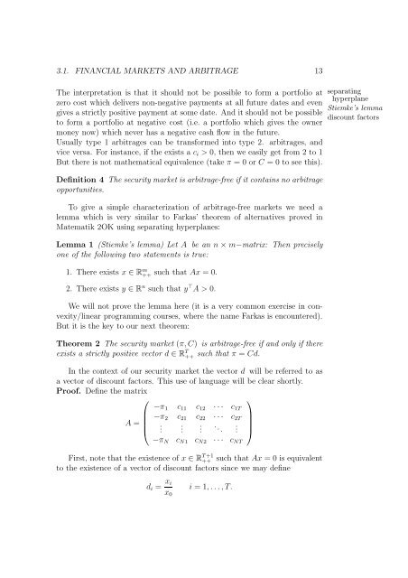
3.1. FINANCIAL MARKETS AND ARBITRAGE 13
The interpretation is that it should not be possible to form a portfolio at
zero cost which delivers non-negative payments at all future dates and even
gives a strictly positive payment at some date. And it should not be possible
to form a portfolio at negative cost (i.e. a portfolio which gives the owner
money now) which never has a negative cash flow in the future.
Usually type 1 arbitrages can be transformed into type 2. arbitrages, and
vice versa. For instance, if the exists a ci > 0, then we easily get from 2 to 1
But there is not mathematical equivalence (take π = 0 or C = 0 to see this).
Definition 4 The security market is arbitrage-free if it contains no arbitrage
opportunities.
To give a simple characterization of arbitrage-free markets we need a
lemma which is very similar to Farkas’ theorem of alternatives proved in
Matematik 2OK using separating hyperplanes:
Lemma 1 (Stiemke’s lemma) Let A be an n × m−matrix: Then precisely
one of the following two statements is true:
1. There exists x ∈ Rm ++ such that Ax = 0.
2. There exists y ∈ R n such that y ⊤ A > 0.
We will not prove the lemma here (it is a very common exercise in convexity/linear
programming courses, where the name Farkas is encountered).
But it is the key to our next theorem:
Theorem 2 The security market (π, C) is arbitrage-free if and only if there
exists a strictly positive vector d ∈ RT ++ such that π = Cd.
In the context of our security market the vector d will be referred to as
a vector of discount factors. This use of language will be clear shortly.
Proof. Define the matrix
⎛
⎞
−π1 c11 c12 · · · c1T
⎜ −π2 c21 c22 · · · c2T
⎟
A = ⎜
⎝
.
. . . ..
⎟
. ⎠
−πN cN1 cN2 · · · cNT
First, note that the existence of x ∈ R T+1
++ such that Ax = 0 is equivalent
to the existence of a vector of discount factors since we may define
di = xi
x0
i = 1, . . .,T.
separating
hyperplane
Stiemke’s lemma
discount factors