STA 414S/2104S: Some notes on bias-variance trade-off February ...

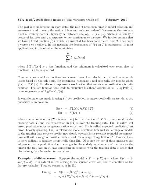
<strong>STA</strong> <strong>414S</strong>/<strong>2104S</strong>: <strong>Some</strong> <strong>notes</strong> on bias-variance trade-off February, 2010The goal is to understand in more detail the role of prediction error in model selection andassessment, and to study the notion of bias and variance trade-off. We assume that we havea set of training data T , typically N instances (x 1 , y 1 ), . . . , (x N , y N ), where x is usually avector of features and y a response, either continuous or discrete. We further assume thatwe have a fitted function ˆf(·), which is a rule that has been constructed from T , that mapsa vector x to a value y. In this notation the dependence of ˆf(·) on T is suppressed. In mostapplications, ˆf(·) is obtained by minimizingN∑L{y i , f(x i )}i=1where L{Y, f(X)} is a loss function, and the minimum is calculated over some class offunctions {f} to be specified.Common choices of loss functions are squared error loss, absolute error, and more rarelylosses based on the pth norm, for continuous responses y and especially for models wheref(x) = E(Y | x). For discrete responses a loss function that counts misclassifications is quitecommon. The loss function that leads to maximum likelihood estimation is −2 log Pr(Y ; θ)or more generally −2 log Pr(Y ; f(·)).In considering errors made in using ˆf(·) for prediction, or more specifically on test data, twoquantities of interest areErr T = E{L(Y, ˆf(X)) | T }, (1)Err = E(Err T ) (2)where the expectation in (??) is over the joint distribution of (Y, X), conditional on thetraining data T , and the expectation in (??) is over the training data. Err T is called testerror, prediction error or generalization error, and Err is called expected prediction/testerror. Loosely speaking, Err T is relevant to model selection: how well will a range of modelsto the training data serve to predict new data?, whereas Err is relevant to model assessment:how well will a range of possible models work for a range of applications? However, Err Tis more difficult to analyse theoretically than Err. Of course neither of these measures canaddress errors in prediction due to changes in the underlying structure of the data or theerrors; the test data must have something in common with the training data in order thatthe training data be useful for prediction.Example: additive errors. Suppose the model is Y = f(X) + ɛ, where E(ɛ) = 0,var(ɛ) = σ 2 ɛ . It is natural in this setting to use squared error loss, and to condition on thefeature variables. Thus we compute, as in §7.3,Err(x 0 ) = E{(Y − ˆf(x 0 )) 2 | X = x 0 }= σ 2 ɛ + {E( ˆf(x 0 )) − f(x 0 )} 2 + var{f(x 0 )},1

In the text in (7.12) the squared bias term is included, but for this particular example it iszero.Example: ridge regression. In the same linear model, if we have ˆβ = (X T X +λI) −1 X T y,then E ˆf(x 0 ) = x T 0 (X T X + λI) −1 X T Xβ and var( ˆf(x 0 )) = x T 0 (X T X + λI) −1 x 0 σ 2 ɛ , and it is atleast plausible that there is some value of λ for which Err(x 0 ) is smaller than its value whenλ = 0.We now consider the estimation of Err in more general settings. The training error is definedaserr = 1 N∑L(y i ,Nˆf(x i )),i=1and it is clearly an underestimate of Err, because ˆf(·) is usually determined to minimize err.In §7.4 the “in-sample generalization error”, or “in-sample test error” is defined asErr in = 1 N∑E{L(Yi 0 ,Nˆf(x i )) | T },i=1where the expectation is over a new sample of Y ’s of size N; one Y for each x i . This is stillconditional on x 1 , . . . , x N . It can be shown thatE y (Err in − err) = 2 N∑cov(y i ,Nˆf(x i ))for both squared error loss and 0-1 loss, and that this holds approximately for log-likelihoodloss. 1 Further, for ˆf(x i ) determined by linear regression with d basis functions, the secondterm is (2/N)dσɛ 2 . This could be simple least squares regression as above, with d = p, orit could be any type of regression spline, or regression on wavelet basis. More generally, asstated in §7.6, ∑ Ni=1 cov(y i, ˆf(x i )) = trace(S)σɛ 2 , for a linear model and any linear fittingmethod ˆf = Sy, which includes regularization methods such as spline smoothing and ridgeregression.This result gives a way to correct err to give an estimate of Err in : sincethen an estimate of the LHS is given byi=1E y (Err in ) = E y (err) + 2 N dσ2 ɛ ,err + 2 N dσ2 ɛ .It is further claimed that for log-likelihood loss, it can be shown that as N → ∞,−2E{log Pr(y; ˆθ)} ≃ − 2 N∑log Pr(y i ;Nˆθ) + 2 d N1 Here E y means expectation over the training y 1 , . . . , y N This is similar to the calculation that takesErr T to Err, but emphasizes via the notation that the training x’s are fixed.3i=1

where d is the number of parameters in ˆθ, thus motivating the estimating the expected lossby the RHS, which is Akaike’s information criterion AIC: see, e.g. (7.30) (where howeverthere is a typo: σ 2 ɛ should not be in the equation).A different derivation of AIC is given in Davison (2003, §4.7), tied more closely to maximumlikelihood fitting. Suppose we have a random sample Y 1 , . . . , Y N from an unknown truedensity g(y), but that we fit the family of models {f(y; θ); θ ∈ Θ} by maximizing the loglikelihoodfunction l(θ) = Σ log f(y i ; θ). Define the Kullback-Liebler discrepancy∫D(f θ , g) =log{ g(y)f(y; θ)}g(y)dy;this is 0 if f(y; θ) = g(y) and otherwise is positive. Denote by θ g the value of θ that minimizesD(f θ , g). The expected likelihood ratio statistic for comparing g with f θ at θ = ˆθ for a newrandom sample Y 1 + , . . . , Y + N from g, independent of Y 1, . . . , Y N is[ N{ }]∑E g+ g(Y +i )logf(Y +i ; ˆθ)= nD(fˆθ, g) ≥ nD(f θg , g).Davison shows thati=1nD(fˆθ, g) . = nD(f θg , g) + (1/2)tr{(ˆθ − θ g )(ˆθ − θ g ) T I g (θ g )},where I g = −n ∫ {∂ 2 log f(y; θ)/∂θ∂θ T }g(y)dY and E g is over the distribution of ˆθ. He thenshows that this can be estimated by−l(ˆθ) + c,where c estimates (1/2)tr{(ˆθ − θ g )(ˆθ − θ g ) T I g (θ g )}, and finally shows that c = p = dim(θ) isthe the expected value of this quantity, so serves as a reasonable estimator. This gives theestimator−l(ˆθ) + p,the AIC is typically a scalar multiple of this. Our book uses the multiple (2/N); other booksuse 2.Finally, a seemingly more direct estimate of ERR T is the cross-validation estimateCV ( ˆf) = 1 N∑L{y i ,Nˆf −κ(i) (x i )},i=1where ˆf −κ(i) (x i ) is the prediction of y i based on a fitted model that omits either the partitionκ(i) that y i falls in (K-fold cross-validation), or simply the ith observation (leave-one-outcross-validation). This would seem to give an internal estimate of Err T , but the book arguesthat in fact it seems to estimate Err instead. For linear smoothers and squared-error loss itcan be shown thatCV = 1 N∑ {y i − ˆf(x i )} 2;N (1 − S ii ) 2i=1replacing (1 − S ii ) by 1 − tr(S)/N makes computations even simpler. This latter expressionis known as the GCV criterion.4