Flexible modelling using basis expansions (Chapter 5) Linear ...

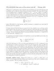
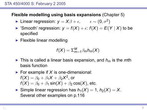
STA 450/4000 S: February 2 2005Flexible modelling using basis expansions (Chapter 5)◮ Linear regression: y = Xβ + ɛ, ɛ ∼ (0, σ 2 )◮ ’Smooth’ regression: y = f (X) + ɛ: f (X) = E(Y | X) to bespecified◮ Flexible linear modellingf (X) = Σ M m=1 β mh m (X)◮ This is called a linear basis expansion, and h m is the mthbasis function◮ For example if X is one-dimensional:f (X) = β 0 + β 1 X + β 2 X 2 , orf (X) = β 0 + β 1 sin(X) + β 2 cos(X), etc.◮ Simple linear regression has h 1 (X) = 1, h 2 (X) = X.Several other examples on p.116: , 1

Regression splines◮ Polynomial fits: h j (x) = x j , j = 0, . . . , m◮ Fit using linear regression with design matrix X, whereX ij = h j (x i )◮ Justification is that any ’smooth’ function can beapproximated by a polynomial expansion (Taylor series)◮ Can be difficult to fit numerically, as correlation betweencolumns can be large◮ May be useful locally, but less likely to work over the rangeof X◮ (rafal.pdf) f (x) = x 2 sin(2x), ɛ ∼ N(0, 2), n = 200◮ It turns out to be easier to find a good set of basis functionsif we only consider small segments in the X-space (localfits)◮ Need to be careful not to overfit, since we are using only afraction of the data: , 2

Regression splines◮ Constraints on derivatives can be incorporated into thebasis: {1, X, X 2 , X 3 , (X − ξ 1 ) 3 + , . . . , (X − ξ k) 3 + } thetruncated power basis◮ procedure: choose number (K ) and placement of knotsξ 1 , . . . ξ K◮ construct X matrix using truncated power basis set◮ run linear regression with ?? degrees of freedom◮ Example: heart failure data from Chapter 4 (462observations, 10 covariates): , 4

Regression splines> bs.sbp dim(bs.sbp)[1] 462 4 # this is the basis matrix> bs.sbp[1:4,]1 2 3 4[1,] 0.16968090 0.4511590 0.34950621 0.029653925[2,] 0.35240669 0.4758851 0.17002102 0.001687183[3,] 0.71090498 0.1642420 0.01087580 0.000000000[4,] 0.09617733 0.3769808 0.44812470 0.078717201: , 5

Regression splines◮ The B-spline basis is hard to described explicitly (seeAppendix to Ch. 5), but can be shown to be equivalent tothe truncated power basis:◮ In R library(splines): bs(x, df=NULL, knots=NULL,degree=3,intercept=FALSE,Boundary.knots=range(x))◮ Must specify either df or knots. For the B-spline basis, #knots = df - degree (degree is usually 3: see ?bs).◮ The knots are fixed, even if you use df (see R code)◮ Natural cubic splines have better endpoint behaviour(linear) (p.120, 121)◮ ns(x, df=NULL, knots=NULL,degree=3,intercept=FALSE,Boundary.knots=range(x))◮ For natural cubic splines, # knots = df - 1: , 6

Example: heart dataRegression splines (p.120) refers to using these basismatrices in a regression model.> ns.hr.glm summary(ns.hr.glm)Call:glm(formula = chd ˜ ns.sbp + ns.tobacco + ns.ldl + famhist +ns.obesity + ns.alcohol + ns.age, family = binomial, data = hr)Deviance Residuals:Min 1Q Median 3Q Max-1.7245 -0.8265 -0.3884 0.8870 2.9588Coefficients:Estimate Std. Error z value Pr(>|z|)(Intercept) -2.1158 2.4067 -0.879 0.379324ns.sbp1 -1.4794 0.8440 -1.753 0.079641 .ns.sbp2 -1.3197 0.7632 -1.729 0.083769 .ns.sbp3 -3.7537 2.0230 -1.856 0.063520 .ns.sbp4 1.3973 1.0037 1.392 0.163884ns.tobacco1 0.6495 0.4586 1.416 0.156691ns.tobacco2 0.4181 0.9031 0.463 0.643397ns.tobacco3 3.3626 1.1873 2.832 0.004625 **ns.tobacco4 3.8534 2.3769 1.621 0.104976ns.ldl1 1.8688 1.3266 1.409 0.158933ns.ldl2 1.7217 1.0320 1.668 0.095248 .ns.ldl3 4.5209 2.9986 1.508 0.131643ns.ldl4 3.3454 1.4523 2.304 0.021249 *famhistPresent 1.0787 0.2389 4.515 6.34e-06 ***ns.obesity1 -3.1058 1.7187 -1.807 0.070748 .: ,ns.obesity2 -2.3753 1.2042 -1.972 0.048555 *ns.obesity3 -5.0541 3.8205 -1.323 0.1858717

Example: heart dataThe individual coefficients don’t mean anything, we need toevaluate groups of coefficients. We can do this with successivelikelihood ratio tests, by hand, e.g.> summary(glm(chd˜ns.sbp+ns.ldl+famhist+ns.obesity+ns.alcohol+ns.age,+ family=binomial, data=hr)) # I left out tobacco... stuff omittedNull deviance: 596.11 on 461 degrees of freedomResidual deviance: 469.61 on 440 degrees of freedomAIC: 513.61Number of Fisher Scoring iterations: 5> 469.61-457.63[1] 11.98> pchisq(11.98,4)[1] 0.9824994> 1-.Last.value[1] 0.01750061 # doesn’t agree exactly with the book, but closeSee Figure 5.4: , 8

Example: heart dataThe function stepAIC does all this for you:> ns.hr.step #> # Here we are at Table 5.1; note that alcohol has been dropped from the> # model: , 9

The function stepAIC does all this for you:> ns.hr.step #> # Here we are at Table 5.1; note that alcohol has been dropped from the> # model2005-02-08Example: heart dataThe degrees of freedom fitted are the number of columns in thebasis matrix (+ 1 for the intercept). This can also be computed as thetrace of the hat matrix, which can be extracted from lm. There issomething analogous for glm, because glm’s are fitted usingiteratively reweighted least squares.

Smoothing splines◮ This is an approach closer to ridge regression. Put knots ateach distinct x value, and then shrink the coefficients bypenalizing the fit . (Figure 5.6)◮subject to:argmin βΣ i(yi − Σ j β j h j (x i ) ) 2β T Ωβ < c◮ with no constraint we get usual least squares◮ Ω controls the smoothness of the final fit:∫Ω jk = h j ′′ (x)h′′ k (x)dx◮ This solves the variational problemargmin fΣ i (y i − f (x i )) 2 + λ∫ ba{f ′′ (t)} 2 dt◮ the solution is a natural cubic spline with knots at each x i

Smoothing splines◮ How many parameters have been fit?◮ It can be shown that the solution to the smoothing splineproblem gives fitted values of the formŷ = S λ y◮ By analogy with ordinary regression, define the effectivedegrees of freedom (EDF) astrace S λ◮ Reminder: ridge regressionmin Σ N i=1 (y i − β 0 − β 1 x i1 − · · · − β p x ip ) 2 + λΣ pβj=1 β2 j⇐⇒ minβΣ N i=1 (y i − β 0 − β 1 x i1 − · · · − β p x ip ) 2 s.t. Σ p j=1 β2 j ≤ shas solutionŷ ridge = X(X T X + λI) −1 X T y: , 12

Smoothing splines◮ In the smoothing case it can be shown thatŷ smooth = H(H T H + λΩ H ) −1 H T ywhere H is the basis matrix. See p. 130, 132 for details onS λ , the smoothing matrix.◮ How to choose λ?◮ a) Decide on df to be used up, e.g.smooth.spline(x,y,df=6), note that increasing dfmeans less ’bias’ and more ’variance’.◮ b) Automatic selection by cross-validation (Figure 5.9): , 13

Smoothing splinesA smoothing spline version of logistic regression is outlined in§5.6, but we’ll wait till we discuss generalized additive models.An example from the R help file for smooth.spline:> data(cars)> attach(cars)> plot(speed, dist, main = "data(cars) & smoothing splines")> cars.spl (cars.spl)Call:smooth.spline(x = speed, y = dist)Smoothing Parameter spar= 0.7801305 lambda= 0.1112206 (11 iterations)Equivalent Degrees of Freedom (Df): 2.635278Penalized Criterion: 4337.638GCV: 244.1044> lines(cars.spl, col = "blue")> lines(smooth.spline(speed, dist, df=10), lty=2, col = "red")> legend(5,120,c(paste("default [C.V.] => df =",round(cars.spl$df,1)),+ "s( * , df = 10)"), col = c("blue","red"), lty = 1:2,+ bg=’bisque’)> detach(): , 14