Final Report - Strategic Environmental Research and Development ...

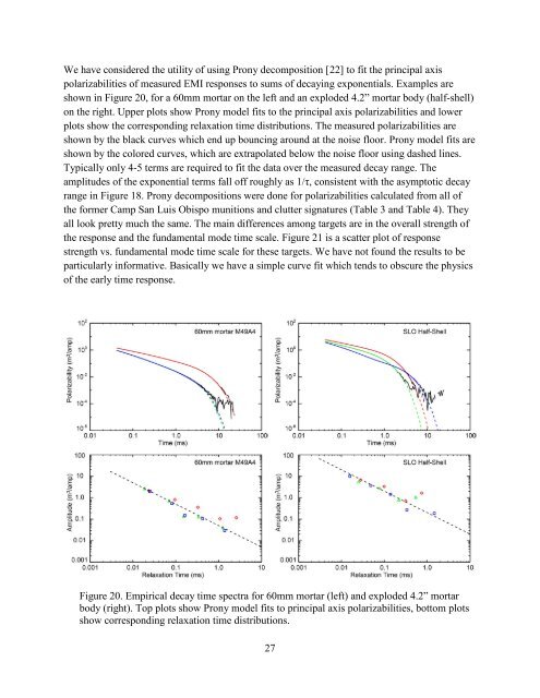
We have considered the utility of using Prony decomposition [22] to fit the principal axispolarizabilities of measured EMI responses to sums of decaying exponentials. Examples areshown in Figure 20, for a 60mm mortar on the left and an exploded 4.2” mortar body (half-shell)on the right. Upper plots show Prony model fits to the principal axis polarizabilities and lowerplots show the corresponding relaxation time distributions. The measured polarizabilities areshown by the black curves which end up bouncing around at the noise floor. Prony model fits areshown by the colored curves, which are extrapolated below the noise floor using dashed lines.Typically only 4-5 terms are required to fit the data over the measured decay range. Theamplitudes of the exponential terms fall off roughly as 1/τ, consistent with the asymptotic decayrange in Figure 18. Prony decompositions were done for polarizabilities calculated from all ofthe former Camp San Luis Obispo munitions and clutter signatures (Table 3 and Table 4). Theyall look pretty much the same. The main differences among targets are in the overall strength ofthe response and the fundamental mode time scale. Figure 21 is a scatter plot of responsestrength vs. fundamental mode time scale for these targets. We have not found the results to beparticularly informative. Basically we have a simple curve fit which tends to obscure the physicsof the early time response.Figure 20. Empirical decay time spectra for 60mm mortar (left) and exploded 4.2” mortarbody (right). Top plots show Prony model fits to principal axis polarizabilities, bottom plotsshow corresponding relaxation time distributions.27