BATHYMETRIC UNCERTAINTY MODEL FOR THE L-3 KLEIN 5410 ...
BATHYMETRIC UNCERTAINTY MODEL FOR THE L-3 KLEIN 5410 ...
BATHYMETRIC UNCERTAINTY MODEL FOR THE L-3 KLEIN 5410 ...
- No tags were found...

Create successful ePaper yourself
Turn your PDF publications into a flip-book with our unique Google optimized e-Paper software.
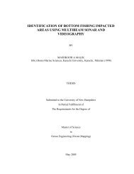
<strong>BATHYMETRIC</strong> <strong>UNCERTAINTY</strong> <strong>MODEL</strong><strong>FOR</strong> <strong>THE</strong> L-3 <strong>KLEIN</strong> <strong>5410</strong> SIDESCAN SONARBYMARC STANTON MOSERB.S. Oregon State University, 1994<strong>THE</strong>SISSubmitted to the University of New HampshireIn Partial Fulfillment ofThe Requirements for the Degree ofMaster of ScienceInOcean EngineeringMay, 2009
Figure 19: Bottom and surface multipath angle calculation showing surface andbottom angles. Bottom noise distance (s BN ) and surface noise distance (s SN )equals signal path distance (s signal ). Bottom noise angle (θ BN ) and signalnoise angle (θ SN ) is a function of sensor depth (z sensor ), depth (z) and signaldistance....................................................................................................... 43Figure 20: Noise source vs signal source for 5-m and 20-m depths assuming asensor depth of one meter and zero sound speed gradient ........................ 44Figure 21: Probability density function (pdf) of phase difference error fromequation (95) for source at bore sight, (70°), noise from surface reflection(117°) at different SNR from equation (103). Decreases in SNR result in themean of the pdf shifting towards the noise solution and increasing standarddeviation...................................................................................................... 45Figure 22: Probability density functions of phase error for three different elementspacing from equation (95) where the source is at boresight (70°), phase foreach pair shown with the black line, and noise from surface reflection(117°), phase for each pair shown with the red line..................................... 45Figure 23: Theoretical effect of pulse bandwidth on the athwartships areaensonified and the vertical measurement.................................................... 47Figure 24: Histogram of depth difference data for single angular sector (69.75° to70.25°)......................................................................................................... 51Figure 25: Histogram of estimated angular error for single angular sector (69.75°to 70.25°)..................................................................................................... 52Figure 26: Estimated angular uncertainty assuming all observed uncertaintiesare the result of the sonar angular uncertainty ............................................ 53Figure 27: Calculated angular uncertainty for gravel (a), sand (b), and bedrock(c), for data without multipath negative sound speed gradient artifacts....... 56Figure 28: Calculated angular uncertainty for negative gradient multipath forgravel (a) and sand (b) ................................................................................ 58Figure 29: Calculated angular uncertainty for gravel (a), sand (b), and bedrock (c)by angle of incidence on the seafloor .......................................................... 59Figure 30: Extrapolated angular uncertainty model based on data acquired oversand showing the original data (squares) along with the model data (pointsand pluses).................................................................................................. 60Figure 31: Top figure showing surface depth for single ping. Bottom figureshowing total vertical uncertainties at 2σ for single ping showing exportedCARIS HIPS, and calculated angular uncertainty model results withobserved uncertainty ................................................................................... 61Figure 32: Theoretical total vertical uncertainty for ideal <strong>5410</strong> for altitudes of 5-mand 20-m showing null at nadir and IHO standards for each depth............. 62Figure 33: Theoretical vertical uncertainty for a <strong>5410</strong> with a DC bias. Neitherdepth range meets IHO Special Order, and only a portion of the swath meetsIHO Order 2................................................................................................. 64Figure 34: Theoretical total vertical uncertainty at 15-m altitude for ideal <strong>5410</strong>with Applanix POS M/V 320 using DGPS correctors (a), Applanix POS M/V320 using RTK (b), and Applanix POS M/V Elite with improved sound speedprofile conditions (c) showing range in predicted performance to IHO Order 1v
standards out to 66 m for (a), IHO Order 1 out to 71 m for (b), and IHO Order1 out to 81 m for (c) ..................................................................................... 66Figure 35: Reduced uncertainty tree for fixed sonar (After Hare, et al. (1995) andCalder (2006)) ............................................................................................. 72Figure 36: Sound speed cast compilation where the DOY of the cast is shown inthe graph at a depth of 30 m ....................................................................... 84Figure 37: Sound speed, temperature, and salinity of casts. Deepest points ofeach salinity and temperature profiles were extrapolated ........................... 85Figure 38: Acoustic backscatter negative sound speed profile gradient multipathinterference for the starboard side out to 100 m. The left is nadir and theright is the farthest away from the sonar. The wavy structures to the rightare due to interference, (DOY 213 in Figure 36) ......................................... 85Figure 39: Receive beam pattern correction (from Glynn, 2007)....................... 87Figure 40: Flowchart of proposed processing steps to solve for sonaruncertainties using multibeam echosounder (MBES) data as a referencesurface......................................................................................................... 91vi
LIST OF TABLESTable 1: Sidescan line spacing based on range scale and coverage ................ 67Table 2: Maximum speed for complete bathymetric coverage........................... 69vii
ABSTRACT<strong>BATHYMETRIC</strong> <strong>UNCERTAINTY</strong> <strong>MODEL</strong><strong>FOR</strong> <strong>THE</strong> L-3 <strong>KLEIN</strong> <strong>5410</strong> SIDESCAN SONARByMarc Stanton MoserUniversity of New Hampshire, May, 2009The L-3 Klein <strong>5410</strong> sidescan sonar system acquires acoustic backscatterimagery and bathymetry data. A bathymetry uncertainty model was developedfor this sonar to predict its performance against hydrographic standardsset by the International Hydrographic Organization (IHO). Elements of the modelnot specific to this sonar were adapted from existing uncertainty models, and theremainder was calculated by comparing the <strong>5410</strong> bathymetry with a referencesurface obtained from multibeam echosounder data. The sonar's angularuncertainty was solved for different bottom types with best results obtained oversandy bottoms, where, after removal of some system biases, the bathymetry metstandards for hydrographic surveys Order 1 from 30º to 75º from nadir. Themodel predicts that the total propagated uncertainty at 20-m altitude meets IHOstandards over a swath width equal to seven times the water-depth, with acentral gap one water-depth wide for an ideal <strong>5410</strong>.viii
INTRODUCTIONThe problem:The L-3 Klein <strong>5410</strong> is one of a number of phase differencing sonars (PDS)manufactured by different vendors and used for seafloor mapping. Whethercalled interferometric [1-6], bathymetric sidescan [7-18], multi-angle swathbathymetry [19, 20], phase measuring sidescan [21], phase interferometry [22],or phase differencing sonar [23], these sonars have the common attribute ofusing one or more pairs of receivers to measure the phase difference of anincoming bottom return to calculate the angle of arrival and two-way travel time.Although these systems share some basic characteristics with widely usedmultibeam echosounders and sidescan sonars, differences in the way a depthmeasurement is determined mean that bathymetric uncertainty models specific tomultibeam echosounders are not necessarily representative of the uncertaintyfrom PDS.Overall goals:a) Evaluate vertical sounding uncertainty for all sources but <strong>5410</strong> sonaruncertaintiesb) Compare calculated with observed <strong>5410</strong> vertical uncertaintyc) Derive a <strong>5410</strong> uncertainty model from residual uncertaintiesd) Evaluate the <strong>5410</strong> uncertainty model against seafloor mapping specifications1
CHAPTER 1OVERVIEW1.1 L-3 Klein <strong>5410</strong> descriptionThe L-3 Klein <strong>5410</strong> phase differencing sonar (PDS) is a modified versionof the popular L-3 Klein series 5000 sidescan sonar, which is used in manyseafloor mapping activities. The addition of two receive and one synthetic(created from four sidescan array elements) bathymetry elements on each sideenables the <strong>5410</strong> to acquire bathymetry [14]. The measured echo phase andmagnitude from the bathymetry element pairs allow the calculation of range andangle of arrival estimates, which together are used to calculate depth and depthposition. The system as studied used a continuous wave (CW) pulse at twodifferent pulse duration settings and is now known as a “version 1” of this <strong>5410</strong>sonar.The acoustic backscatter imagery from the L-3 Klein 5000 series has a0.20–0.36 m along track and 0.075–0.300 m across track resolution [24]. Thisresolution meets the International Hydrographic Organization (IHO) featuredetection criteria for a one meter cubic object [25] provided the sonar is operatedto maximize feature detection.2
The analyzed <strong>5410</strong> is jointly owned by the National Oceanic andAtmospheric Administration (NOAA) Office of Coast Survey (OCS) and NationalMarine Fisheries Service (NMFS). Personnel at the University of NewHampshire (UNH) Center for Coastal and Ocean Mapping / Joint HydrographicCenter (CCOM/JHC) have been working with the <strong>5410</strong> for a number of years. Amethod to convert the raw SDF formatted data into a format usable by CARISHIPS software as well as a calibration procedure developed by Glynn [14]enabled the bathymetry of the <strong>5410</strong> to be used for seafloor mapping. Separatelyfrom CCOM/UNH, Zerr et al. [26] also acquired and processed <strong>5410</strong> bathymetryfor rapid environment assessment. CARIS HIPS is a commercially availablepackage to process hydrographic data [27], specifically seafloor mapping dataused primarily for nautical charting and safety of navigation purposes. In thisproject, a timing method described by Calder and McLeod [28] was also utilizedfor improved data acquisition. A proof of concept survey in New York Harborwas successfully completed in late 2006 [13]. Newer versions of the processingcode were developed by James Glynn, Christian de Moustier, and Brian Locke in2007 and 2008.1.2 Previous work with uncertaintyThe total uncertainty for the bathymetric solution of the <strong>5410</strong> can bebroken into two parts: sonar specific uncertainty and uncertainty from everyother source. The uncertainty from every other source has been investigatedand described by Hare, et al. [29, 30]. Theoretical PDS uncertainties including3
the effects of shifting foot print [11, 12, 19], baseline decorrelation [11, 12, 19],multipath and ambient noise [8, 16], and volume reverberation [7] have also beenexplored. In general, these theoretical PDS uncertainties have a detrimentaleffect on the angle of arrival solution. Other sonar specific uncertainties alsoinclude the impact of processing methods on the angle of arrival solution and theuncertainties associated with the sonar characteristics including pulse duration,acoustic frequency, pulse type, and the effect of environmental conditions on theangle of arrival solution.Performance and uncertainties for sonar bathymetry have been evaluatedfor non <strong>5410</strong> PDS systems. Gostnell et al. [5, 31] evaluated the bathymetry froma Geoacoustics Geoswath, a SEA Swath Plus, and a Teledyne Benthos 3D.Hogarth [32] derived an uncertainty model for the Geoacoustics Geoswath. Hilleret al. [33] examined modifying the Combined Uncertainty and BathymetryEstimator (CUBE) for use with PDS bathymetry.1.3 Benefits of bathymetric uncertainty modelThe primary benefit of a bathymetric uncertainty model for the <strong>5410</strong> is toenable potential users to determine whether the system meets certain criteria forseafloor mapping. Other benefits of a <strong>5410</strong> uncertainty model include pre-surveyplanning and bathymetric data processing. Calder and Mayer [34] developed amethod to process large bathymetric data sets utilizing uncertainty (CUBE). Anuncertainty model for the <strong>5410</strong> bathymetry would allow the use of CUBE forprocessing <strong>5410</strong> data.4
CHAPTER 2ANGLES AND OFFSETSBefore discussing the uncertainty equations it is necessary to define thesource and definition of major components used in those calculations. Sonarsystems are composed of several sensing components that are typicallyseparated from each other on the moving echosounding platform. Cleardefinitions of offsets and rotations between components are needed to utilize theattitude output from the motion sensor, while the methodology for ray tracing andangle of incidence calculations are important for the uncertainty calculations andlater analysis.2.1 Offsets, coordinate systems and rotationsOffsets are described using the three axis system shown in Figure 1. TheY offset is positive forward, the X offset is positive to starboard, and the Z offsetis positive down (into the water) in this context. X, Y, and Z offsets are themeasured distances from the top of the IMU center mark to the phase center ofeach sonar transducer. Rotations around these axes are defined using the righthandcoordinate system conventions.5
Figure 1: R/V Coastal Surveyor offsetsAttitude data were acquired using a rotation convention called Tait-Bryan[35, 36]. The sequence for Tait-Bryan rotations is yaw-pitch-roll (Ф,Γ,Ψ). Apositive rotation around the Z axis is clockwise. A positive rotation around the Yaxis is port up. A positive rotation around the X axis is bow up. An example Tait-Bryan sequence is shown Figure 2, with positive yaw, pitch, and roll rotations.Figure 2: Tait-Bryan rotation sequence showing yaw (a), pitch (b), and roll (c)6
The Tait-Bryan sequence can be used with rotation matrices to describeand quantify the position of the sonar at any given time. Goldstein [37] derivesthe matrices to describe these rotations.⎛1 0 0⎜R( Ψ ) = 0 cosΨatt−sinΨ⎜⎝0 sinΨattcosΨ⎛ cos Γatt0 sin Γ⎜R( Γ ) = 0 1 0⎜⎝−sin Γatt0 cos Γattattattatt⎞⎟⎟⎠⎛cos Φatt−sin Φatt0⎞⎜⎟R( Φ ) = sinΦattcosΦatt0⎜ 0 0 1⎟⎝⎠⎞⎟⎟⎠( 1)( 2)( 3)2.2 Vertical offsetsFor ray tracing, the vertical position of the sensor transducer with respectto the water surface at the time of reception (z sensor ) is calculated using the totalheave (H), the static draft (Ds), dynamic draft (Dd), and the vertical offset of thesensor to the reference point (Z), which are illustrated in Figure 3. Static draft isthe vertical offset of the reference point (in this case the attitude sensor) to thewater surface when the vessel is underway but not making way (i.e. drifting, notmoored). Dynamic draft is the vertical offset of the reference point to the watersurface when the vessel is underway and making way. Most vessels have adynamic draft that depends on their speed through the water. The vertical offset(Z) is the measured vertical offset from the attitude sensor (top of the IMU) to thephase center of the sonar. Total heave is a combination of measured heave at7
the attitude sensor and induced heave. Measured heave is the verticalmovement of the attitude sensor. Induced heave is the apparent verticalmovement of the sonar with respect to the attitude sensor due to vesselrotations. The sensor vertical position is used for ray tracing, reduced depthcalculation and uncertainty calculations.zsensor= Z − Ds+ Dd + H( 4)Another vertical change not directly measured or applied is the change invessel vertical position under different loading conditions. These include using ortaking on fresh water, ballast, fuel, passengers, and equipment. Normally thesechanges would be taken into account with frequent static draft measurements.Figure 3: Vertical position of sonar calculated from: (a) static draft, (b) dynamic draft, (c)heave, (d) and (e) induced heave8
The rotational matrices can be reduced to calculate a sonar position for agiven set of angles. When the rotation matrices are multiplied with a vector ofoffsets, the result is the rotated sonar position as shown by Hare, et al. [29]. Therotations assume that the rotated body is rigid and there is no flexing or changeof the offsets during the rotation.⎡Y⎤ ⎡YRot⎤R( Φ) R( Γ) R( Ψ )⎢X⎥ ⎢X⎥⎢ ⎥= ⎢ Rot ⎥( 5)⎢⎣Z⎥⎦ ⎢⎣Z⎥Rot ⎦Since yaw (Ф) is irrelevant for the calculation of induced heave, the Yawrotation matrix becomes an identity matrix.⎛1 0 0⎞⎛ cosΓ 0 sin Γ⎞⎛cos Ψ −sin Ψ 0⎞⎡Y⎤ ⎡YRot⎤⎜ ⎟⎜ ⎟⎜ ⎟0 1 0 0 1 0 sinΨ cosΨ 0⎢X⎥=⎢X⎥Rot( 6)⎟⎜ ⎟⎜ ⎢ ⎥ ⎢ ⎥⎜0 0 1⎟⎜ sin 0 cos ⎟⎜ 0 0 1⎟ ⎝ ⎠⎝− Γ Γ⎠⎝ ⎠⎣ ⎢Z⎥⎦ ⎢⎣ Z ⎥Rot ⎦The rotation matrices can further be reduced to solve for induced heave.Induced heave is calculated using Pitch (Γ att ), Roll (Ψ att ), and offsets of the sensorfrom the attitude sensor (X, Y, Z) [29]:( )Hind = ⎡⎣−Ysin( Γatt) + X sin( Ψatt )cos( Γatt) + Z 1−cos( Ψatt )cos( Γatt) ⎤⎦ ( 7)Total heave (H) includes the heave at the attitude sensor (H att ) and theinduced heave resulting from the motion of the vessel (H ind ).H = H + H( 8)attindThe measured depth (z) and sensor depth (z sensor ) and give the depth ofwater at the time of acquisition. The water depth at time of acquisition canfurther be reduced to a common vertical datum. Reduction of water depths to acommon datum are necessary for comparison of depth data acquired at different9
times. The most common vertical datum for NOAA nautical charts is mean lowerlow water (MLLW), which was used for the test data. Tide measurements (Tides)from the NOAA tide gauges used for this analysis were relative to MLLW.z = z + z− Tides( 9)redsensorSince most data were acquired away from the NOAA tide gauges it wasnecessary to utilize tide zoning to approximate the tides at the geographiclocation of acquisition. Simple tide zones generated by NOAA for previoushydrographic surveys were used for the tide zoning [38]. The total tide correctionwas designed to match as closely as possible with the method used by CARISHIPS [27] so comparison of depth results and surfaces exported from CARISHIPS would reflect as closely as possible the results calculated independently.Although more advanced methods of tide correction have been developed [39],these methods were not used for this analysis.The vessel position was evaluated for each ping to determine in which tidezone polygon it resided. Each tide zone polygon was attributed with a range andtime corrector. Measured tide data were then corrected for the time andmultiplied by the range ratio for the final tide correction, which is consistent withNOAA’s hydrographic survey procedures. Tide data from NOAA gauges inPortsmouth, NH (842-3898) and Portland, ME (841-8150) were used.Although the Portsmouth, NH, tide gauge is very close to the survey areaand would have been preferable for all data, it was inoperative for a period oftime during data acquisition and the Portland gauge was used for a portion of thedata. This should not affect the validity of results.10
2.3 Launch angle determinationSince the raw angle of echo arrival reported by the <strong>5410</strong> is with respect tothe sonar reference frame, the angle must be converted to an angle with respectto vertical for ray tracing in the water column. The launch angle of a given ray isdetermined using the raw angle of arrival (θ Raw ) with respect to the sonarreference frame, measured roll and pitch, and biases. The angle of arrival ismeasured from vertical with a value of zero at nadir, -90° to port and 90° tostarboard. Pitch (Γ) and roll (Ψ) angles are a combination of the measuredvalues (Γ att ,Ψ att ) at the attitude sensor and their respective bias (Γ bias ,Ψ bias ). Theangle of arrival is measured at the instant when the transmitted sound has madea round trip to the bottom and attitude values are evaluated at the arrival time.Γ=Γ −Γ ( 10)attattbiasΨ=Ψ −Ψ ( 11)biasUsing the law of sines for tetrahedra, the corrected angle of arrival (θ Corr )can be calculated using the raw angle of arrival (θ Raw ), pitch (Γ), and roll (Ψ). Allof the triangles of the tetrahedron are right triangles and four of the angles (Γ,(90°-Γ), (θ+Ψ), (90°-(θ+Ψ))) are known. With the notation given in Figure 4, thelaw of sines states:sin OAB sin OBC sin OCA = sin OAC sin OCB sin OBA ( 12)Where OAB = 90°, OBC = 90 °− ( θ Raw+Ψ ) , OCA = 90°−Γ, OAC = 90°, OCB = 90° andOBA = 90 °− θCor. Equation (12) becomes:( θ )sin 90° sin 90° sin(90 °− θ ) = sin 90° sin 90 °− ( +Ψ ) sin(90 °−Γ )( 13)CorrRaw11
Reducing equation (13) results in the solution for the corrected angle ofarrival:( θ )sin(90 °− θ ) = sin 90 °− ( +Ψ ) sin(90 °−Γ )( 14)Corr( θ )Rawcos( θ ) = cos +Ψ cos( Γ )( 15)θCorrCorrRaw−= cos cos( Γ )cos( +Ψ )( 16)1[ θ ]RawFigure 4: Solution for corrected angle of arrival through law of sines for tetrahedrawhere the corrected angle of arrival (θ Corr ) is AOB, pitch (Γ) is AOC, the raw angle ofarrival and roll (θ raw + Ψ) is COB. OAB, OAC, OCB, and ACB are right angles.2.4 Ray tracingEchosounding pulses from the <strong>5410</strong> travel obliquely through the watercolumn. The speed at which sound travels through water column varies withdepth. The depth, traveled range, and horizontal range are calculated usingeither a constant sound speed gradient method [40] or a zero gradient method.To match the application method used in CARIS HIPS [27], sound speed profileswere selected based on the time difference between the sound speed cast andthe survey line and the distance of the cast to the line. The cast nearest in12
distance and time (within three hours) was selected. Most casts acquired for thisproject have a first entry at around one meter depth. Each cast was extrapolatedto the surface for ray tracing using a pressure only gradient. Another option, thatconsists of extrapolating from the slope of the profile deeper than one meter wasnot used based on the assumption that the top one meter of the water columnwould be relatively well mixed.Cast data also have a finite measured depth. The last measured point isextrapolated to the seafloor by the NOAA cast processing software Velocwin [41]using the ‘most probable slope algorithm’ method. This Velocwin extrapolatedpoint is at times not deep enough for all rays, so an additional point is generatedin Matlab using an isothermal gradient (0.017 s -1 ) to a depth known to be greaterthan the maximum survey area depth.Using the extended cast data, ray tracing for each solution is calculated,depending on the measured sound speed gradient, using either the constantgradient solution or zero gradient solution. The corrected angle of arrival atreceive (θ Corr ) is evaluated at the measured sensor depth (z sensor (Rx)) at the timeof arrival. Subsequently, the average sensor depth between transmit (Tx) andreceive (Rx) is used to determine the sensor depth (z sensor ) in equation (9).zsensorzsensor( Tx) + zsensor( Rx)2= ( 17)For simplicity, the depth increments in the sound speed cast are used forall but the final layer for layer calculations. A layer is a horizontal slice of theocean with a constant vertical gradient, assuming that there is no horizontalsound speed gradient. The gradient (g i ) for a given layer is calculated using the13
difference in the top and bottom depths of the layer (Δz i ) and the difference in thespeed of sound at the top (c i ) and bottom (c i+1 ) of the layer.gi=( c c )− i+ 1ΔziiIf the gradient does not approach zero, the constant sound speed gradient( 18)solution is used to solve for the ray path. The ray parameter, or Snell’s Lawconstant of the ray (p) is given by the corrected angle at receive (θ Corr ) and thespeed of sound at the sensor (c sensor ) [40]. This ray parameter is constant for theentire ray path and is derived using Snell’s Law.p( θ ) sinθ θ θ+ 1sin sin sinc c c cCorr 2i i= = = = ( 19)sensor 2 i i+1The radius of curvature (R i ) for a given layer is given from the rayparameter (p) and gradient (g i ) in that layer. The radius of curvature is constantwhile the gradient is constant.Ri1p( g )= ( 20)iThe angle of incidence for the top layer (θ i ) and bottom layer (θ i+1 ) arecalculated using Snell’s law, the speed of sound at the sensor (c sensor ), top of layer(c i ) and bottom of layer (c i+1 ).⎡−⎛ c ⎞⎤θi = sin ⎢sin( Corr) ⎜ ⎟⎥= sin (i)⎣ ⎝csensor⎠⎦θ1 i−θ1[ p c ]= sin⎡sin(⎛)c ⎞⎤= sin ( )⎣ ⎝ ⎠⎦1 i+1−θ1[ pc ]−i+ 1 ⎢ Corr ⎜ ⎟⎥i+1csensor( 21)( 22)14
The horizontal distance traveled by the ray (r hi ) shown in Figure 5 is givenby the ray parameter (p), gradient (g i ), speed of sound at the top of the layer (c i ),and depth difference of the layer (Δz i ).rhi( ) ⎤ ( )2 21 − ⎡⎣p ci +Δzi( gi) ⎦ − 1 − p( ci)= ( 23)pg ( )iFigure 5: Constant negative sound speed gradient layer ray traceThe distance traveled by the ray (s i ) is given by the radius of curvature (R i )and the difference in angle of incidence in radians from the top (θ i ) and bottom(θ i+1 ) of the layer:s = R( θ − θ )( 24)i i i+1 iThe travel time of the ray (t i ) through layer i is given by the gradient (g i ),sound speed at the top of the layer (c i ), depth difference of the layer (Δz i ), andthe ray parameter (p).ti=1gi⎡⎢⎢⎢⎣( c + g Δ z )(1+ 1 −( p( c ))i i i i( )ci(1+ 1− ⎡⎣p ci + giΔzi⎤⎦22⎤⎥⎥⎥⎦( 25)15
As an iterative process, the sum of the travel times through each layer isevaluated against one half of the total recorded two-way travel time (t f ).IftNf− ∑ ti> 0 then continue to next full layer ( 26)2Elsei=1tNf− ∑ ti< 0 then evaluate from last full layer ( 27)2i=1The remaining component of the solution is to solve for the partial layer,where the ray hits the bottom between depth increments of the sound speedprofile. The sum of travel times (t i ) up to the last full layer (N-1) is subtractedfrom half the recorded two way travel time (t f /2) for the remaining time (t r ).trtN −1f= −∑ ti( 28)2 i=0The remaining travel time (t r ) is then used to solve the angle of incidenceat the bottom (θ r ) using the gradient of the final layer (g N ), and the angle ofincidence at the top of the layer (θ N-1 ).tr1 ⎡ tan( θ / 2) ⎤lnr= ⎢ ⎥gN⎣ tan( θN− 1 / 2) ⎦Therefore,( 29)θ =⎡⎣⎤⎦ ( 30)−1tgr2tan tan( θN−1/2) er N16
Figure 6: Constant sound speed ray tracing solution for partial layerThe remaining horizontal distance (r hr ) can then be solved using the radiusof curvature (R N ), and the angle of incidence of the top (θ N-1 ) and bottom (θ r ) ofthe partial layer in radians.[ cos( ) cos( )]r = R θ − θ( 31)hr N N−1rThe remaining distance traveled (s r ) is solved using the radius of curvature(R), and the angle of incidence of the top (θ N-1 ) and bottom (θ r ) of the partial layerin radians to calculate the arc distance.[ ]sr RN θr θN− 1= − ( 32)The remaining depth difference (Δz r ) is solved using the radius ofcurvature (R N ), angles of incidence at the top (θ N-1 ) and bottom (θ r ):[ sin sin ]zr R θr θN− 1Δ = − ( 33)If the gradient is very small in layer i, the gradient (g i ) approaches zeroand the radius of curvature (R i ) approaches infinity. Under these circumstances,the constant sound speed gradient solution cannot be used and the zero gradient17
solution must be used. Then the horizontal distance (r hi ) traveled by the ray isgiven by the depth difference (Δz i ) and angle of incidence (θ i ):r =Δ z tan( θ )( 34)hi i iThe distance traveled (s i ) is given by the depth difference (Δz i ) and angleof incidence (θ i ):siΔzi= ( 35)cos( θ )iFigure 7: Zero gradient layer ray traceThe travel time (t i ) is given by the depth difference (Δz i ), sound speed (c i )and angle of incidence (θ i ).ti⎛ Δz⎞i= ⎜ ⎟/ci( 36)⎝cos( θi) ⎠As with the constant sound speed gradient method, remaining time (t r ) isused to solve for the remaining partial layer. The depth difference (Δz r ) iscalculated using the angle of incidence (θ N-1 ), remaining travel time (t r ), andsound speed (c N-1 ).18
Δ z = c t( 37)rcos( θN − 1)N − 1 rThe remaining horizontal distance is calculated using the depth difference(Δz r ) and angle of incidence (θ N-1 ).r =Δ z tan( θ )( 38)hr r rThe remaining distance traveled (s r ) is calculated using the depth difference (Δz r )and angle of incidence (θ N-1 ).srΔzcos( )= ( 39)rθN− 1For all of the layers traveled by the ray, the sums of the travel times (t i:N-1 +t r ), distance traveled (s i:N-1 + s r ), layer thickness (Δz i:N-1 + Δz r ), and horizontaldistance (r h i:N-1 + r hr ) provide the final solutions for total distance traveled (s),horizontal range (r h ), and depth below the sensor (z).2.5 Angle of incidence on the seafloorThe angle of incidence of a ray on the seafloor can be used in the depthuncertainty equations and can also be used to determine the existence of anyangle of incidence dependence in the <strong>5410</strong> depth uncertainty. The calculation ofthe angle of incidence uses the angle of impact (angle of incidence before bottomslope correction) of a given ray to a hypothetical horizontal bottom using Snell’sLaw and the slope of the bathymetric surface at the point of impact, expressedusing the surface normal and the ray vector [42]. For a givensurface f ( N, E, z ) = 0, where Northing (N), Easting (E), and depth (z) are19
provided, the surface normal and direction cosines can be calculated for thatsurface as follows:Each component of the normal vector can be broken down using thepartial derivatives of the surface function f. ⎡∂f ∂f ∂f⎤u = ⎢, ,⎣∂N ∂E ∂z⎥⎦( 40)The direction cosines of the normal vector ( , , )the normalized individual components (N, E, z) of u .L M N are calculated fromu u uLuuuN= ( 41)MuuuE= ( 42)Nuuzu= ( 43)Where u is the norm of u :u = u + u + u( 44)2 2 2N E zFor a given ray, where the azimuth angle and final angle of incidence withrespect to a hypothetical horizontal bottom are provided, the direction cosines ofthe ray vector v can be calculated.The azimuth of a ray vector is calculated from the vessel heading (Ф) anda corrector. Since these rays are pointing towards (not away) from the source,the resultant azimuth angle for port (Ф port ) and starboard (Ф stbd ) are reversed.20
ΦportΦstbd=Φ+ 90=Φ+ 270( 45)( 46)Figure 8: Azimuth angles for port and starboard raysThe azimuth (Ф port and Ф stbd ) and initial angle of incidence (θ init ) of each rayare used to calculate the normal for the ray.v = v sinθsin Φ ( 47)Einitv = v sinθcos Φ ( 48)Ninitv = v cosθ( 49)zinitWhere v is used to normalize the results to calculate the direction cosines (L v ,M v , and N v ) for the ray vector.v = v + v + v( 50)2 2 2E N zLvvvN= ( 51)MvvvE= ( 52)Nvvzv= ( 53)21
The final angle of incidence (θ Inc ) is calculated by using the surface normal u andray vector v .θInc−1uNvN uvE Euvz z= cos ⎡ ⎢ + +⎤⎥⎣ uv uv uv⎦Equation (54) can be expressed as the inner product of normal vectors( 54)shown in equation (55).( ) ( )= − ⎡ ⎣⋅ ⎤ ⎦1θ Inccos u v / u v( 55)Figure 9: Angle of incidence components for ray vector (a), surface normal (b), andresulting angle of incidence (c)22
CHAPTER 3<strong>UNCERTAINTY</strong>Chapter 2 defined the basic building blocks for the values utilized in theuncertainty equations. With these definitions the total propagated uncertaintycan now be calculated for <strong>5410</strong> data. Once the uncertainties for all but the sonarare calculated and the difference data of the <strong>5410</strong> and multibeam referencesurface are calculated, the <strong>5410</strong> uncertainty model can be calculated.3.1 Uncertainty calculationsUncertainty calculations for all uncertainty with the exception of the sonarwere derived from the equations documented from Hare, et al. [29, 30]. Theseequations were appropriate for the <strong>5410</strong> analysis since the components of theuncertainty equations appeared to match those of the processing software [27]used to create the bathymetric surfaces in this analysis, allowing for a directcomparison of calculated uncertainty values against a known standard.3.1.1 Discussion on uncertainty values usedUncertainty values used were either directly obtained from vendorspecifications, laboratory testing, or best estimates based on availableinformation. Uncertainty values provided by the vendors included thoseuncertainties associated with vessel motion and positioning [43, 44] and sonar23
characteristics [45]. Some uncertainty values for those sonar characteristics notprovided by the vendor were observed from laboratory testing by Glynn [14]. Theremaining non-sonar uncertainties were estimated from observations andguidance from relevant standards [3, 23, 25].This analysis uses baseline sound speed and tide uncertainty values thatare lower than recommended by NOAA specifications [3, 23], because observeduncertainties were less than the uncertainties calculated by CARIS HIPS.Uncertainties for draft were also estimated and the resulting baseline values arelower than recommended by NOAA. The uncertainty values used in the Matlabcode written for this analysis were the same as those used in CARIS HIPS forevery uncertainty except for the <strong>5410</strong> uncertainties. A listing of uncertaintyvalues used in both applications is shown in Appendix C.Multibeam echosounder biases are normally resolved for time, pitch, yawand roll. It should be noted that the only practical bias that could be resolvedwith the <strong>5410</strong> data used here were roll bias values. Since there are no data atnadir, solving for pitch and navigation time delay biases is difficult. Due to thevery precise timing system used during acquisition, timing uncertainties wereassumed to be minimal. Yaw was also difficult to solve since the data acquiredfor the purpose of solving for that bias were degraded due to negative soundspeed gradient multipath artifacts. Therefore, other bias values including yawand navigation time were not solved but were assumed to be zero. As discussedby Hughes Clark [46], a misalignment around the z axis of the roll and pitch axesof the attitude sensor would result in cross talk between measured roll and pitch24
values. This cross talk would be visible as a heave artifact. Since yaw is notbeing included in these calculations, the links between yaw, pitch, roll, andinduced heave will not be discussed further.3.1.2 Uncertainty propagationThe method for uncertainty propagation considered here is based on aTaylor Series expansion of the multivariate uncertainty function [46, 47]. Theuncertainty for a function j F( k,l)= composed of two independent and randomvariables (k,l) can be described as the sum of products of the squared partialderivatives and variances of each variable.2 22 ⎛ ∂j⎞ 2 ⎛∂j⎞2j=k+lσ ⎜ ⎟kσ ⎜ ⎟⎝∂⎠ ⎝∂l⎠σIf the two variables (k,l) are not independent, then an additional term(covariance) must also be considered as part of the total uncertainty equation.( 56)2 22 ⎛ ∂j ⎞ 2 ⎛ ∂j ⎞ 2 ⎛j k l2∂j ⎞⎛ ∂j⎞= + +klσ ⎜ ⎟ σ ⎜ ⎟ σ ⎜ ⎟⎜ ⎟σ⎝∂k ⎠ ⎝∂l⎠ ⎝∂k ⎠⎝∂l⎠( 57)Whereσklis the covariance of k and l.Based on the uncertainty equations from Hare, et al. [29, 30], it wasassumed that all of the uncertainty calculations can be used for the <strong>5410</strong> datawith the exception of the depth/sonar equations which are system specific.3.1.3 Range and Bearing estimationSince the angle of arrival and total range for each ray (calculated from raytracing) are not usually the straight line bearing and range used in the uncertaintymodel by Hare, et al. [29, 30], it is necessary to compute the corresponding25
estimated straight line bearing (θ bearing ) and range (r est ). The straight line bearingcan be calculated using the horizontal range (r h ) and depth (z).θbearing−1⎡rh⎤= tan ⎢ z ⎥( 58)⎣ ⎦Since the straight line bearing is the result of pitch and across trackcomponents, the bearing must be broken into separate pitch and across trackcomponents to use the uncertainty equations described by Hare, et al. [29, 30].Using equation (16) and the estimated straight line bearing and pitch, theestimated athwartships component of the straight line bearing can be calculated.θest= cos−1⎡ ⎛ −1⎡rh⎤⎞⎤⎢cos⎜tan⎢ ⎥z ⎥⎟⎢ ⎝ ⎣ ⎦⎠⎥⎢ cos( Γ)⎥⎢⎥⎣⎦The r h used to calculate the bearing should not be confused with the( 59)Cartesian coordinates used for the offsets. The horizontal range (r h ) as used inequation (59) and shown in Figure 10 is a directionless value and does notcorrespond with the usual definitions of x and y as across and along trackcomponents of a ray tracing solution or Easting and Northing positioncoordinates.26
Figure 10: Difference between corrected angle of arrival (θ Corr ), absolute bearing (θ Bearning ),and athwartships bearing component (θ est )r = r + z( 60)est2 2hThe effective straight line sound speed for each ray (c est ) can be calculatedfrom the measured two-way travel time (t f ) and estimated straight path range(r est ).cestrest= ( 61)( tf/2)Assuming that the difference between the combination of pitch andestimated bearing (cos(Γ)cos(θ est )) and the corrected angle of arrival (θ Corr ) issmall, the depth uncertainties associated with the estimated bearing should beequal to the depth uncertainties associated with the corrected angle of arrival.3.1.4 Non-sonar uncertainty equationsThe critical path for <strong>5410</strong> depth uncertainty analysis is highlighted in red inFigure 11. Using the observed difference data as a proxy for the reduced depthand measured depth uncertainties, the uncertainty equations can be reversed tocalculate the desired sonar characteristics. Besides the direct relationships27
etween uncertainty components, possible correlation (covariance terms) areillustrated using dashed lines. This diagram and the following equations aremeant to address only those sources of uncertainty specific to this data set anddo not address other sources of uncertainty associated with some multibeamechosounders (i.e. uncertainty due to beam steering). Other sources ofuncertainty, which are not specifically addressed, include the effect of yawuncertainty on pitch and roll and the ultimate effect on heave [46]. Other possiblesources of uncertainty correlation will be addressed with the specific uncertaintyequations.28
Figure 11: Uncertainty tree (After Hare, et al. (1995) and Calder (2006)). Uncertainties notbeing displayed include cross-terms for yaw uncertainty and heave, roll and pitchuncertainty on refraction, and heave uncertainty on refractionThe reduced depth uncertainty is the combination of the depthmeasurement uncertainty (σ Dmeas ), tide uncertainty (σ Tides ), and draft (σ Draft ).These three uncertainty components are uncorrelated; therefore the reduceddepth variance is shown below without covariance terms.σ = σ + σ + σ( 62)2 2 2 2Dred Dmeas Tides DraftAlthough it could be argued that an uncertainty in the draft would affectsome components of the depth measurement uncertainty (by having a directimpact on the depth of the sonar for ray tracing), it is assumed such acontribution would be extremely small for these data and will therefore beignored.29
The draft uncertainty is the combination of the uncertainty of dynamic draft(σ DynDraft ), static draft (σ StaticDraft ), and loading (σ Loading ). As described in section2.2, each of the draft uncertainty components has a unique definition andconsequentially they are considered uncorrelated. Although it is possible that byimproperly modeling one draft component, the remaining components would beaffected (i.e. not taking into account the change in static or dynamic draft due tosignificant loading condition changes), it is assumed that the draft components ofthe R/V Coastal Surveyor are well understood, measured, and modeled for thetest data.σ = σ + σ + σ( 63)2 2 2 2Draft DynDraft StaticDraft LoadingThe tide uncertainty is the combination of the tide gauge measurementuncertainty (σ TideMeas ) and the uncertainty associated with the tide zoning(σ TideZone ). The uncertainty of the tide gauge is wholly independent of the zoningcomponent.σ = σ + σ( 64)2 2 2Tides TideMeas TideZoneDepth measurement uncertainty is the combination of depth/pitchuncertainty (σ DΨ ), depth/roll uncertainty (σ DΓ ), depth/heave uncertainty (σ Dheave ),depth/sonar uncertainty (σ Sonar ), depth/refraction uncertainty (σ Dref ), andcovariance terms for heave, pitch and roll and refraction.Starting with the covariance terms, the Roll term of induced heave is:⎛∂Dmeas⎞⎜ ⎟ = Ψ Γ − Ψ Γ⎝ ∂DhvΨ⎠( X cos( )cos( ) Zsin( )cos( ))att att att att( 65)30
The Roll term of depth:⎛ ∂Dmeas⎜⎞ ⎟ = Γest est⎝ ∂DΨ⎠( r cos( θ )cos( ))Pitch from induced heave:( 66)⎛∂Dmeas⎞⎜ ⎟ = ( Ycos( Γatt) − X sin( Ψatt)sin( Γatt) − Zcos( Ψatt)sin( Γatt))⎝ ∂DhvΓ⎠Pitch term of depth:( 67)⎛ ∂Dmeas⎜⎞ ⎟ = Γest est⎝ ∂DΓ⎠( r cos( θ )sin( ))Pitch and roll from refraction:( 68)⎛ ∂Dmeas⎞ ⎛cos( θest) cos( Γ)⎞⎜ ⎟= ⎜ ⎟⎝∂DrefΓΨ⎠ ⎝ cest⎠Heave from refraction:( 69)⎛∂Dmeas⎞ ⎛sin( θest) ⎞⎜ ⎟ = ⎜ ⎟⎝ ∂Dhv⎠ ⎝ cest⎠To calculate the covariance terms for Pitch, Roll, depth and heave:( 70)= 1∑ ( D Γ − D Γ )( hv Γ − hv Γ )( 71)nσD Γ hv Γn i=1i i= 1∑ ( D Ψ − D Ψ )( hv Ψ − hv Ψ )( 72)nσD Ψ hv Γn i=1i iTo calculate the covariance terms for Pitch, Roll, heave, and refraction:= 1( D Γ − D Γ )( ref Γ − ref Γ )nσD Γ ref ΓΨn i=1i i∑ ( 73)= 1∑ ( D Ψ − D Ψ )( ref Ψ − ref Ψ )( 74)nσD Ψ ref ΓΨn i=1i iσn1= ∑ ( Dhv −Dhv)( refhv −refhv)( 75)Dhvrefhv i in i=131
The covariance terms can be included in the measured depth uncertaintycalculation, shown in equation (76). Although it is possible, under certaincircumstances, that the covariance terms would be important for measured depthuncertainty, it is unlikely that the covariance terms would have a significant effectfor this test data and will be ignored for calculation of the <strong>5410</strong> uncertainty model.Combining these terms with the individual uncertainty components results in thedepth measurement uncertainty:σ2Dmeas⎡σ + σ + σ + σ + σ + σ⎢⎢ ⎛⎛∂Dmeas⎞⎛∂Dmeas⎞⎞⎢ ⎜⎜ ⎟⎜ ⎟σ⎟DΓhvΓ⎢ ⎜⎝ ∂DΓ ⎠⎝ ∂hvΓ⎠ ⎟⎢ ⎜⎟∂Dmeas∂Dmeas⎢ ⎜ ⎛ ⎞⎛ ⎞+ ⎜ ⎟⎜ ⎟ σ ⎟DΨhvΨ⎢ ⎜ ⎝ ∂DΨ ⎠⎝ ∂hvΨ⎠ ⎟= ⎢ ⎜⎟⎢ ⎛∂Dmeas⎞⎛∂Dmeas⎞+ 2⎜+ ⎜ ⎟⎜ ⎟σ⎟DΓrefΓΨ⎢ ⎜ ⎝ ∂DΓ ⎠⎝ ∂refΓ⎠⎟⎢ ⎜⎟⎢ ⎜ ⎛∂Dmeas⎞⎛∂Dmeas⎞ ⎟⎢ ⎜+ ⎜ ⎟⎜ ⎟σDΨrefΓΨ⎝ ∂DΨ ⎠⎝ ∂refΨ⎟⎢ ⎜⎠ ⎟⎢ ⎜ ⎛∂Dmeas⎞⎛∂Dmeas⎞ ⎟⎢ ⎜+ ⎜ ⎟⎜ ⎟σDhvrefhv⎝ ∂Dhv⎠ ∂refhv⎟⎣⎢⎝⎝ ⎠ ⎠2 2 2 2 2 2DΨDΓDheave Dbw Dsonar DrefDepth/Roll uncertainty is calculated from the estimated range, bearing andthe roll uncertainty:⎤⎥⎥⎥⎥⎥⎥⎥⎥⎥⎥⎥⎥⎥⎥⎥⎥⎦⎥( 76)( r sin( )cos( )) 2σ = θ Γ σ( 77)2 2DΨest estΨDepth/Pitch uncertainty is calculated from the estimated range, bearingand pitch uncertainty:( r cos( )sin( )) 2σ = θ Γ σ( 78)2 2DΓest estΓ32
Depth/Heave uncertainty is the combination of the measured and inducedheave.σ = σ + σ( 79)2 2 2Dheave InducedHeave MeasuredHeaveInduced heave uncertainty is the combination of pitch, roll, offsets, pitchuncertainty, roll uncertainty, and offset measurement uncertainties.σ2inducedHeave2 2⎡( Ycos( Γatt ) − X sin( Ψatt )sin( Γatt ) −Zcos( Ψatt )sin( Γatt)) σΓ+ ⎤⎢⎥2 2⎢( X cos( Ψatt )cos( Γatt ) −Zsin( Ψatt )cos( Γatt) σΨ+ ⎥= ⎢ 2 2 2 2(sin(att)) σY (sin(att)cos(att)) σ⎥⎢Γ + Ψ ΓX⎥⎢2 2⎣+ (1−cos( Ψatt ) cos( Γatt )) σ⎥Z⎦Breaking up the heave uncertainty into different components, the heaveand pitch components of heave can be used for covariance analysis.( 80)σ = σ + σ + σ( 81)σσ2 2 2 2InducedHeave hvΨhvΓhvOff( X cos( )cos( ) Zsin( )cos( )) 2= Ψ Γ − Ψ Γ σ( 82)2 2hvΨatt att att att Ψ( Ycos( ) X sin( )sin( ) Zcos( )sin( )) 2= Γ − Ψ Γ − Ψ Γ σ( 83)2 2hvΓatt att att att att Γ( sin( )) ( sin( )cos( )) ( 1 cos( )cos( ))2 2 2 2 2 2 2hvOff att Y att att X att att Zσ = Γ σ + Ψ Γ σ + − Ψ Γ σ ( 84)Pitch uncertainty is the combination of the sensor pitch measurementuncertainty and the uncertainty of the pitch bias estimate.σ = σ + σ( 85)2 2 2Γ ΓmeasΓalignRoll uncertainty is the combination of the sensor roll measurementuncertainty and the uncertainty of the roll bias estimate.σ = σ + σ( 86)2 2 2Ψ ΨmeasΨalign33
According to the manufacturer of the heave sensing unit, the heaveuncertainty is the larger of either (a) a fixed component of heave or (b) apercentage of the measured heave.( a bHmeas)σ = max ,( )( 87)2 2 2MeasuredHeaveDepth/Beamwidth uncertainty is calculated from the fore-aft beamwidth(ε Y ) and depth below the sensor (z).σ2Dbw⎡ ⎛ ⎛εY⎞⎞⎤= ⎢z⎜1−cos⎜⎟ ⎥2⎟⎣ ⎝ ⎝ ⎠⎠⎦2Depth/Sonar uncertainty is the unknown and will be calculated fromobserved difference data in a later section.( 88)σ =< UNKNOWN > ( 89)DsonarDepth/Refraction uncertainty is calculated from the estimated range,bearing, pitch, estimated ray sound speed, and sound speed uncertainty.2 2 22⎛rest cos( θ ) ⎞2⎛estrest sin( θ ) ⎞ ⎡est ⎛tan( θest) ⎞ 2Dref ⎜ cos( ) ⎟ cp ⎜ cos( ) ⎟ ⎜ ⎟ cpcestcest⎝ 2 ⎠⎤σ = Γ σ + Γ ⎢ σ ⎥⎝ ⎠ ⎝ ⎠ ⎢⎣ ⎥⎦( 90)The total propagated uncertainties of all sources of uncertainty exceptthose for the sonar can be calculated for individual soundings and forhypothetical scenarios. The total and individual uncertainties for all sources ofuncertainty except the sonar are shown in Figure 12, assuming a scenario similarto that used during acquisition of the test data and a 20-m altitude.34
Figure 12: Total vertical uncertainty and individual uncertainties at 2σ without sonaruncertainties at 20-m altitude3.2 Calculation of observed difference dataOnce the uncertainties for all but the sonar are calculated, the next stepneeded to solve for the <strong>5410</strong> uncertainties is the calculation of difference data.Processed hydrographic data cleaning system (HDCS) data were exported fromCARIS HIPS into a text format that was then imported into Matlab. Text files ofsurfaces created from <strong>5410</strong> PDS data and Kongsberg EM 3002 data were alsoexported from CARIS HIPS and imported into Matlab. Each surface was aregularly spaced grid, with equal Easting and Northing facets. Grid resolution isdefined as the length of a full side of any given square cell (a one meterresolution grid cell has a length of one meter and a width of one meter). The gridnode of a cell is the center of that cell. Each sounding position (Easting andNorthing) was evaluated against grid node positions to find the nearest grid node35
within a maximum horizontal radius (r Max ). The maximum radius term was used,consequently only grid cells in the vicinity of the sounding position wereevaluated. In Figure 13, z Diff is the vertical difference between the sounding(z sounding ) and the grid node depth (z grid ) and γ is the grid resolution. Grid cellswere considered as horizontal entities. A negative value indicates that thesounding is shoaler than the grid node. A positive value indicates that thesounding is deeper than the grid node.zDiff = zcaris − zgrid( 91)rMax2= 2γ( 92)Although <strong>5410</strong> bathymetry data were manually edited in CARIS HIPS forgross errors for surface creation, all <strong>5410</strong> bathymetry were exported to Matlaband considered for analysis.Figure 13: Determination of vertical difference between sounding and grid node using thegrid resolution (γ) to determine the maximum search radius (r max ) for finding the nearestgrid node for each sounding36
3.3 Mean difference between <strong>5410</strong> soundings and reference surfaceTo determine if any systematic uncertainty was present in the differencedata (z Diff ), the mean for any given angular sector (θ a ) can be calculated. Angularsectors are defined as all of the data with raw angle of arrival values within thebounds of the sector (i.e. 59.75° to 60.25°).zn1( θ ) = ∑ z( 93)Diff a Diff in i=1If no systematic uncertainty were present in the data, one would expectthe mean of each angular sector to approach zero as more data are evaluated.This was not the case for the reviewed <strong>5410</strong> bathymetry. The mean for anygiven angular sector varied from line to line. As the results from multiple lineswere summed, the mean of most sectors did not approach zero.To perform uncertainty analysis using the difference data, it wasnecessary to remove the difference bias in the data so only random error wasconsidered. The mean of each angular sector (z filter (θ a )) for a given line wassubtracted from the observed difference (z Diff ) to calculate the corrected observeddifference (z zeromean ).z ( θ ) = z ( θ ) − z ( θ )( 94)zeromean a Diff a filter aA number of non-sonar sources of uncertainty that would be relativelyconstant for a single line would be extracted by removal of the mean. Tide anddraft systematic errors would be extracted by removal of the mean. Anysystematic bias from the sonar or sonar processing would also be extracted byremoval of the mean. A modification to the processing code developed by Locke37
educed some of the mean bias for the port data, but not the starboard data.Because port and starboard data show different biases, this suggests that thebiases are at least partially sonar specific and not tide or draft induced.Figure 14: Sample mean (black dots) and standard deviation (blue pluses) for 51 linesbinned in 0.5° sectors without filtering shows difference data irregularities. Port data is onthe left and starboard data is on the rightFigure 14 may give the impression that all data showed the exact samefilter results, but this was not the case. Each line had a slightly different angularbin means, with the general trends remaining (i.e. the inflection points at 45° and65° in the starboard data were always visible, but the actual difference valuevaried). Figure 15 shows the results of the individual removed means used foreach line. The data past 70° are not being shown since they were much morevariable. The port side data, in general, had a higher trend (or peak) around 45°.The starboard data shows more defined peaks around 46° and 65°.38
Figure 15: Mean filter results for individual lines. Horizontal axis is the line number andthe vertical axis is angle from nadir. The color is based on the filter value in meters. Notethat the starboard data on the right show peaks around 46° and 65°Figure 16 shows the results of removing each line mean from each line.The data binned by angular sector for all of the lines now have a near zero mean.A discussion on the possible causes will follow later in this section but it shouldbe noted again that a number of non-sonar errors could be removed by thisfiltering method. Those errors that in effect would create a static bias for thepurposes of a single line are tides, draft, and sound speed profile. A distinctionis made between uncertainty (as used in the rest of this document) and errorhere because at this point an estimate exists of the difference between the trueand measured values. The systematic error (or bias) is removed from the data in39
order to analyze the random uncertainties of the data. If the difference data werenot de-trended then the assumption that the sonar uncertainties are randomcannot be made when solving for those uncertainties.Figure 16: Sample mean (black dots) and standard deviation (blue pluses) for 51 linesbinned in 0.5° sectors with filtering. Port data on the left and starboard data on the rightThe difference data can be categorized by bottom type shown in Figure17. Using an existing bottom type map by Ward [48], all individual points for agiven angular bin can be separately evaluated by bottom category. Figure 17shows histogram for three different bottom types for a single angular sector.Although the histograms do vary slightly from each other (slightly differentvariances), the differences may be more the result of sample size rather thanshowing different performance based on bottom type. Angular uncertaintyresults will be evaluated against bottom type in a later section.40
Figure 17: Histograms of de-trended difference data for a single angular bin for 51 lines forgravel (a), sand (b), and bedrock (c) where the red line is the Gaussian fit.There are two hypotheses for the cause of the apparent bias removed byfiltering each line: (1) a meandering DC basis for each element and (2) multipathinterference.In work by Glynn [14], it was assumed that the DC bias of any receiveelement was static and did not change for a given set of data. In that work, thestatic DC bias was removed in processing. The first hypothesis, which has beenproposed by de Moustier (de Mousiter, 2008, Personal Communication), is thatthe DC bias for each channel was not static but changed over time. A non-staticDC bias would have a detrimental effect on the phase difference (and thereforeangle of arrival estimation) solution and would increase the uncertainty. It is alsotrue, but harder to show, that a drifting DC bias could create a constant bias inthe difference data.The second hypothesis is that the difference bias is the result of multipathinterference. Using the technique for determining phase errors due tointerference described by Denbigh [16], the mean and standard deviationanomalies could be explained by back calculating the most likely source of noiseinterference. The probability density function of the phase error can beexpressed as:41
2J ⎡ 1 A ⎧π−1⎫⎤p( ϕ) = sin A4 2 2 3/22πσ⎢ − ⎨ − ⎬1 − A (1 −A) 2⎥( 95)⎣⎩ ⎭⎦Using the simplified assumption derived by Denbigh [16] where P s is thesignal power, P I is the noise power, φ S is the signal phase, and φ I is the noisephase.2σ = Ps+ PI( 96)ρ = P cosϕ + P cosϕ( 97)s s I Iη =− ( P sinϕ + P sin ϕ )( 98)s s I IA η ϕ ρ ϕ σ2= ( sin − cos )/( 99)2 4 2 2J = σ −ρ − η( 100)Assuming that the two way travel time for the interference must match thatof the signal, and that the most likely causes of interference are those paths withthe minimum number of surface or bottom bounces, each given angle of arrivalhas one or two possible noise sources.Figure 18: Multipath noise sources: desired signal path (black line), interferencepaths (red lines). Inset: pair of receivers separated by distance (d)42
Each multipath ray is a sum of two separate rays. Using the zero gradientassumption, each ray leg can be considered a single ray with a single angle ofarrival. Due to the zero gradient assumption, the range traveled by the signal ray(s Signal ) will be the same as the two sources of interference (s BN and s SN ).θθSNBN1 ( 2Sensor)cos⎡ ⎛ − z+z= ⎢−⎞⎥⎤⎢⎜ s ⎟⎣ ⎝ Signal ⎠⎥⎦1 (2Sensor)cos⎡ − z+z= ⎢ ⎤⎥⎢⎣sSignal⎥⎦( 101)( 102)Figure 19: Bottom and surface multipath angle calculation showing surface and bottomangles. Bottom noise distance (s BN ) and surface noise distance (s SN ) equals signal pathdistance (s signal ). Bottom noise angle (θ BN ) and signal noise angle (θ SN ) is a function ofsensor depth (z sensor ), depth (z) and signal distance.The resultant noise source locations are shown in Figure 20 with theoriginal signal source direction. Bottom and surface multiples could have asignificant effect on the mean and standard deviation of the phase differencesolution. The actual geometry for any given ping changes over time (as the43
sonar is deeper or shoaler in the water column and as the vessel moves), butthere is an average sonar depth, roll, and pitch which would be reflected in thephase difference error results.Figure 20: Noise source vs signal source for 5-m and 20-m depths assuming a sensordepth of one meter and zero sound speed gradient3.4 Effect of signal-to-noise ratio (SNR)As the SNR decreases (signal power usually decreases with range andrelative noise power increases), the bias (difference between the expectedsolution and the mean of the calculated phase difference solution) increases.The variance of the phase difference solution also increases as the SNRdecreases. SNR (dB) is calculated from the noise and signal power:SNR10log⎛ P ⎞S=10 ⎜ ⎟PI⎝⎠( 103)Using a single pair of elements as an example, the mean of a phasesolution moves away from zero and the variance increases as the signal to noiseratio decreases. A bias in the phase solution would result in a bias of the angleof arrival solution and would therefore create a bias in the difference data. An44
example probability density function of the phase error is shown for a singleelement pair with different signal to noise values in Figure 21. At lower signal tonoise values the phase error ceases to be centered on zero.Figure 21: Probability density function (pdf) of phase difference error from equation (95)for source at bore sight, (70°), noise from surface reflection (117°) at different SNR fromequation (103). Decreases in SNR result in the mean of the pdf shifting towards the noisesolution and increasing standard deviationComparing three different element distances shown in Figure 22, thephase bias can be different for each element pair.Figure 22: Probability density functions of phase error for three different elementspacing from equation (95) where the source is at boresight (70°), phase for each pairshown with the black line, and noise from surface reflection (117°), phase for each pairshown with the red line45
Although the Denbigh equations do offer an explanation for the resultingdifference data irregularity, the more probable explanation is the non-stationaryof the DC bias. It is highly unlikely that multipath interference for any givenangular region would be consistent enough over time to cause an angular biasfor that angular region. Much more likely is that multipath interference will overtime cause the angular uncertainty for a given angular sector to increase.3.5 Time resolution (pulse bandwidth)The sonar depth uncertainty from the pulse bandwidth is the firstcomponent to be discussed for the <strong>5410</strong>. Pulse bandwidth impacts the rangeuncertainty, which in turn affects the sonar vertical uncertainty. Verticalmeasurement uncertainty due to pulse bandwidth (σ 2 SonarBW) can beapproximated with the angle of incidence (θ Inc ), speed of sound (c), rangesampling distance (Δrs), and the pulse duration (τ) in seconds. Hare et al. [29,30] used the equation below from Hammerstad [49]:2 22 2 rs cτσ SonarBWcos θ ⎛ ⎡ Δ ⎤ ⎡ ⎤= ⎞Inc ⎜ + ⎟⎜⎢ ⎣ 2 ⎥⎦⎢⎣ 4 ⎥⎝⎦⎟⎠( 104)The angle of incidence is being used rather than the bearing and pitchbecause the angle of incidence of a given ray on the seafloor will affect the depthuncertainty from the pulse bandwidth. Figure 23 shows a diagram of the effect ofpulse bandwidth on the area of the seafloor ensonified.46
Figure 23: Theoretical effect of pulse bandwidth on the athwartships area ensonifiedand the vertical measurementUnfortunately, the observed data does not support the results of equation(104) for use with the <strong>5410</strong>. The depth uncertainty from that equation was toolarge and would have adsorbed all of the observed variability (and would haveimplied a null angular uncertainty for most of the swath). The difference betweenthe expected and observed uncertainty can be better explained through thesampling rate. The range sampling is calculated using the sampling frequency( Δ t = 1/ fs), or sampling time interval as:cΔt1500(1/ 22750)Δ rs =Δ Rt= = = 0.033m( 105)2 2The range resolution (ΔR BW ) calculated from pulse bandwidth (BW) is:c 1500Δ RBW= = = 0.15m( 106)2BW2(4800)47
ΔRBWThis means that there are ( ≅ 4.7 ) range samples for each rangeΔRresolution cell. Assuming a uniform distribution of the samples within eachresolution cell whose end points are defined as:tΔR −Δ R⎛ΔR=⎞ΔR⎝ ⎠( )BWtN t0⎜ ⎟ tΔRtthe variance of these samples is:( 107)22 ( ΔRtN−ΔRt0)σX= ( 108)12Therefore,2σ SonarBW2 2 2⎛ c ⎞ ⎛ c ⎞ ⎛ c ⎞= ⎜ ⎟ /12 = ⎜ ⎟ /48 ≅⎜ ⎟⎝2BW ⎠ ⎝BW ⎠ ⎝7BW⎠( 109)A detrimental aspect of the GSF format currently used for the <strong>5410</strong> data isthe time resolution for two way travel time in the test data. From the samplingfrequency (f s ), one would expect a minimum time resolution of 4.4x10 -5 s, but theGSF data analyzed only supported 10 -4 s. Although the GSF format doessupport scale factors [50], they were not utilized in the right way for the test data.It is recommended that for future analysis, the optional scale factor field beutilized correctly for <strong>5410</strong> GSF data to allow increased time resolution.Whenever the sampling rate of the sonar (ΔtSonar) is smaller than the GSF timeresolution (ΔtGSF), the discrepancy introduces a range resolution uncertaintyindependent of the sonar shown as:48
⎡ ⎛ ⎡ 1 ⎤⎞⎤⎢c⎜ΔtGSF−⎢f⎥⎟⎥⎣ s ⎦Δ RGSF=⎢ ⎝⎠⎥⎢/22 ⎥( 110)⎢⎥⎢⎣⎥⎦Combining these two components results in the depth uncertainty due tobandwidth and time resolution:σ⎛ ⎡ ⎛⎤⎞⎤⎜ ⎟ ⎜ ⎟⎜ ⎥⎟⎥⎝⎢⎣⎝ ⎣ ⎦⎠⎥⎦22 2 ⎛ c ⎞ ⎛c⎞⎡ 1SonarBW= cos θ ⎜Inc+ ⎢ ⎜ΔtGSF−⎜⎢⎝7BW⎠ ⎝4⎠fsIf future <strong>5410</strong> GSF format data utilize the two way travel time scale factor,then the second term can be eliminated from future versions of <strong>5410</strong> uncertaintymodels.2⎞⎟( 111)⎟⎠3.6 <strong>5410</strong> Signal ProcessingThe description of the <strong>5410</strong> processing method used by Glynn [14] isimportant in understanding the results of the angular uncertainty that will bepresented in chapter 4. Since the <strong>5410</strong> data are processed using a method thatdiffers from other phase differencing systems, it is reasonable to assume that theangular uncertainty will also be different than predicted from those othermethods.Glynn [14] describes the equations using phasor processing techniques tosolve the differential phase measurements between multiple receivers. Thesame equations can be used to solve for the magnitude from multiple receivers.This is the method used by Locke (Locke, 2008, Personal Communication) afterfiltering the real and imaginary components.49
Glynn [14] filters the real and imaginary components using an FIR filter.The differential phase solution for each bathymetric pair are filtered using avariable length FIR filter that used an increasing number of samples farther out inthe swath after 45°. After filtering, the three phase difference solutions are usedto calculate the angle of arrival. Vector averaging of the three solutions is used,with an angular tolerance, so outlier angle of arrival estimates from a single pairdo not unduly weight the final solution. The reported angle of arrival from theprocessing method should be described as the estimated angle of arrival since itis the product of multiple filtering steps and vector averaging. The practicaleffects of filtering mean that the resulting bathymetry can be much less noisythan data not processed using this method.Lurton has proposed a number of equations describing the angularuncertainty for a system based on the signal to noise ratio [11, 12]. Theseequations were not used due to the differences in processing methods implied inthe Lurton articles and those used for test <strong>5410</strong> data [14]. Lurton also shows asimilar equation utilizing the signal to noise ratio and other data for the sonardepth uncertainty [30]. These equations were not used for this analysis.3.7 Angular UncertaintyThe angular uncertainty is the second component of the sonar depthuncertainty. Angular uncertainty can be approximated using the de-trendedvertical difference data (z zeromean ). Assuming that any angular uncertainty wouldvary for each side and angular sector from nadir, the difference data from50
multiple lines can be evaluated. Figure 24 shows a histogram of de-trendeddepth difference data for a 0.5° bin from multiple lines.Figure 24: Histogram of depth difference data for single angular sector (69.75° to70.25°)The difference between the estimated (θ est ) and observed angles is theapproximation of the angular error. The sample estimate of variance of theangular error is the angular uncertainty. The observed angle could beapproximated by using the measured depth (z), depth difference (z zeromean ), andpitch (Γ).θObserved⎡ ⎡−1⎛ z−z ⎞⎤⎤ ⎡⎡⎛ zeromeanz−z⎞⎤⎤zeromean⎢cos ⎢cos⎜ ⎟⎥⎥ ⎢⎢⎜ ⎟⎥⎥r1 estr−⎝ ⎠ −1⎝ est ⎠= cos⎢ ⎣ ⎦⎥ cos⎢⎣ ⎦⎥⎢=cos( Γ) ⎥ ⎢ cos( Γ)⎥⎢ ⎥ ⎢ ⎥⎢⎣ ⎥⎦ ⎢⎣ ⎥⎦Taking the difference between the estimated and observed angle givesthe estimated angular error. The weakness with using this method to calculatethe angular uncertainty for the sonar is that all sources of uncertainty are beingconsidered as angular uncertainty. This problem is overcome in equation (114)as all of the depth uncertainties are considered before solving for the angular( 112)51
uncertainty. Figure 25 shows a histogram of angular error from the de-trendeddepth difference data from Figure 24.Figure 25: Histogram of estimated angular error for single angular sector (69.75° to70.25°)The variance of the distribution shown in Figure 25 would be the estimatedangular uncertainty for this angular sector. Solving for all angular sectors, anapproximate angular uncertainty model was generated, which is presented inFigure 26.52
Figure 26: Estimated angular uncertainty assuming all observed uncertainties are theresult of the sonar angular uncertaintySince this model represents the cumulative effects of all sources ofuncertainty, it cannot be used as a model solely for the angular uncertainty of the<strong>5410</strong>. A more appropriate approach is to consider the angular uncertainty aspart of a larger set of equations describing the total uncertainty.As derived by Hare, et al. [29], the portion of the sonar uncertainty relatedto the angle solution can be calculated using the estimated range (r est ), estimatedangle (θ est ), pitch (Γ), and the sonar angular uncertainty (σ 2 θ Sonar ). If all of theother uncertainties are known and the observed data uncertainty is known, thenthe sonar angular uncertainty can be solved.( sin cos ) 2σ Sonar = r estθ estΓ σ θ Sonar( 113)2 2θEquations (111) and (113) can be combined for the sonar depthuncertainty shown in equation (114).53
σ2DSounder⎡ ⎛22 c ⎡ c ⎛ 1 ⎞⎤⎢cosθ ⎜⎛ ⎞ ⎛ ⎞ ⎡ ⎤Inc ⎜ ⎟ + ⎢⎜ ΔtGSF−7BW4⎟⎜⎜⎢ ⎥f ⎟⎥= ⎢ ⎜⎝ ⎠ ⎢⎝ ⎠⎝⎣ s ⎦⎠⎥⎢ ⎝ ⎣⎦⎢2 2⎢⎣+ ( s ( sinθest) cos Γ)σ θSonarIt is incorrect to assume that the standard deviation of the difference datafrom each angular sector can be used to solve for the angular uncertainty. Sinceeach bin of de-trended difference data represent a variety of measured depths,ranges, and angles of incidence, all line data were evaluated against thecalculated uncertainties to determine what value for angular uncertainty wouldaccount for 95% or more of the absolute value of the difference data. The crossterms (covariance) were not used in the calculations. Equation (115) was usedto solve for the angular uncertainty.2⎞⎤⎟⎥⎟⎥( 114)⎠⎥⎥⎥⎦⎧1/2⎡ 2 2 2 2 2σDHeaveσDσDσDbwσ Sonar ⎤+Γ+Ψ+ +BWn⎢⎥⎪2 2⎪∑ ⎨z⎢zeromeanσTidesσ⎥Draft⎬ ( 115)i=1⎢⎥10.95 = ≤ 1.96 + + +n ⎪⎪⎢⎩⎣2 2( rest sinθest cos Γ) ( σ θSonar)⎥⎦⎫⎪⎪⎭54
CHAPTER 4RESULTSWith the uncertainty values and difference data calculated in chapter 3,the <strong>5410</strong> angular uncertainty can be modeled. The <strong>5410</strong> angular uncertainty(σ 2 θ Sonar ) was separately determined for each side of the sonar. Data weredivided into short segments along a single track of echosounding and designatedas a line. Each line represented approximately one minute of data and wascategorized by the amount of observed acoustic backscatter imagery artifactscaused by multipath. Imagery artifacts coincided with strongly definedthermocline in the sound speed profiles and are considered separately since theresulting data represent the effect of the environment on the <strong>5410</strong> rather than theperformance of the <strong>5410</strong> when evaluated alone. See Appendix D for informationon sound speed, salinity, and temperature profiles acquired for this test.It should also be noted that the performance of the port and starboardsides differed significantly. Although this difference is carried through in lateranalysis, it is reasonable to expect that any future <strong>5410</strong> PDS systems will haveconsistent performance for both the port and starboard sides. Glynn [14]proposed that observed differences in transducer performance could be theresult of variations in manufacturing methods used when the transducers werebuilt.55
Angular uncertainty values were stratified by bottom type by determiningwhether each sounding resided in specific polygon bottom type regions createdfrom a modified bottom type map from Ward [48]. There were some differencesbetween the gravel and sand data, with greater differences between these twoand bedrock data. Figure 27 shows the calculated angular uncertainty for thethree bottom types. It is apparent that the angular uncertainty increased rapidlyat 70° for both port and starboard gravel data when compared to sand data. Alsoapparent is the greater angular uncertainty for bedrock areas.Figure 27: Calculated angular uncertainty for gravel (a), sand (b), and bedrock (c), fordata without multipath negative sound speed gradient artifacts56
The poor results from the bedrock data have two possible explanations.The first explanation is that the sonar performed poorly over areas where thebottom was complex with respect to the resolution of the reference surfaceresolution (one meter). The second explanation is that the <strong>5410</strong> was recordingthe depths of underwater vegetation growing on the bedrock. No directobservations were made to determine whether vegetation was growing on thebedrock at the time of the experiment. Additional work outside the scope of thisanalysis is necessary to resolve this problem.If the impact of multipath artifacts due to negative sound speed gradient isextrapolated to <strong>5410</strong> bathymetry from acoustic backscatter imagery, it would beexpected that the calculated angular uncertainty out to a coincident angle fromnadir would match that from data without artifacts. Figure 28 shows the angularuncertainty calculated from lines with artifacts classified by bottom type for sandand gravel. The results for sand roughly match that shown in Figure 27 exceptthat the angular uncertainty rapidly increases at 70°. The gravel angularuncertainty for data with artifacts is less well defined but also increases at 70°suggesting that multipath effects after 60° are being observed.57
Figure 28: Calculated angular uncertainty for negative gradient multipath for gravel (a)and sand (b)Angular uncertainty can also be evaluated against the angle of incidencecalculated in Chapter 2. If the <strong>5410</strong> bathymetry has an angular dependencesimilar to that of the acoustic backscatter it would be expected to be apparent inthe angular uncertainty results shown in Figure 29. The angular uncertaintyresults represented here do differ from those shown in Figure 27 but do notnecessarily show distinct incidence angle dependence. The prominent spike inangular uncertainty for gravel in Figure 27 has become more gradual and lessabrupt in Figure 29. Based on these results it cannot be demonstrated that thereis a reduction in bathymetric performance due to a critical angle of incidence.58
Figure 29: Calculated angular uncertainty for gravel (a), sand (b), and bedrock (c) by angleof incidence on the seafloorBased on the unresolved issues associated with results in gravel and rockareas, the angular uncertainty results from the sand data were used. Portions ofthe sand data with no angular uncertainty results were extrapolated near nadirand the outer swath to produce an angular uncertainty model for the <strong>5410</strong>. Thesand data did not have angular uncertainty results out to 90° due to the bottomgeometry of the sand test data and range scale used when compared to theother areas. This model shown in Figure 30 will be used to evaluate potentialsonar performance in the next chapter.59
Figure 30: Extrapolated angular uncertainty model based on data acquired over sandshowing the original data (squares) along with the model data (points and pluses)The total propagated uncertainties from the CARIS HIPS export,calculated angular uncertainty and the observed uncertainties are plotted inFigure 31. In general, the exported CARIS HIPS uncertainty valuesunderestimated the total uncertainty. The starboard angular uncertainty modelshows up in the figure as a distinct peak around 43°.60
Figure 31: Top figure showing surface depth for single ping. Bottom figure showingtotal vertical uncertainties at 2σ for single ping showing exported CARIS HIPS, andcalculated angular uncertainty model results with observed uncertaintyAlthough the exact uncertainty equations utilized by CARIS HIPS are notknown, the differences between the total uncertainty using equation (63) and thatexported from CARIS HIPS are most likely caused by different uncertaintyequations for pulse bandwidth, and angular uncertainty (equation (115)). Theresults for the <strong>5410</strong> angular uncertainty computed in this analysis are consideredmore reflective of actual uncertainty as justified by the analysis.61
CHAPTER 5EVALUATION OF <strong>UNCERTAINTY</strong> <strong>MODEL</strong> WITH OCEANMAPPING STANDARDSAssuming a basic survey scenario similar to that carried out duringacquisition of the test data, the angular uncertainties derived from the sand datacombined with all other sources of uncertainty were used to predict performancefor two different sonar altitude values (5 m and 20 m) representing the normalrange of many NOAA hydrographic surveys, with the results presented in Figure32.Figure 32: Theoretical total vertical uncertainty for ideal <strong>5410</strong> for altitudes of 5-m and 20-mshowing null at nadir and IHO standards for each depth62
The International Hydrographic Organization (IHO) promulgatesuncertainty standards for hydrographic surveys by dividing these standards intocategories or “Orders” appropriate for different navigational situations. SpecialOrder is the most stringent, Order 1 is most broadly applicable, and Order 2applies to less critical areas. Based on Figure 32, one could expect to acquiredata meeting the IHO Special Order criteria out to 38 m from nadir, Order 1 out to50 m, and Order 2 out to 75 m for a sonar altitude of five meters. Increasing thealtitude to 20-m, but keeping all the basic assumptions the same, one couldexpect to acquire data meeting IHO Special Order criteria out to 50 m, Order 1out to 80 m, and Order 2 out to 125 m under the same survey scenario as thatcarried out during the test data acquisition.It may be useful to consider performance in a variety of less than idealcircumstances. Figure 33 shows the theoretical performance of the <strong>5410</strong> if theDC bias is not resolved. The variance and mean results shown in Figure 14 hasbeen re-introduced into equation (63) and the absolute value of the mean addedto the total propagated uncertainty. The performance for both depth rangesappreciably degrades with only a portion of the swath meeting IHO Order 2 forboth depth ranges.63
Figure 33: Theoretical vertical uncertainty for a <strong>5410</strong> with a DC bias. Neither depthrange meets IHO Special Order, and only a portion of the swath meets IHO Order 2.The swath covered by usable bathymetry is usually less than that coveredby usable acoustic backscatter imagery in the test data. In other words, at a 75-m range scale, the <strong>5410</strong> acoustic backscatter imagery reaches out to 75 m, butthe bathymetry may only reach out to 65 m to 70 m.Figure 34 shows three scenarios for total vertical uncertainty for the <strong>5410</strong>for an altitude of 15-m. All sources of uncertainty are the same with theexception of changes to the roll, pitch, heave, and refraction uncertainties.Figure 34 (a) shows the results from using the same attitude sensor as used forthe experiment with the only difference that DGPS correctors rather than RTK isbeing used. The use of DGPS correctors for this attitude sensor increases theuncertainty for roll and pitch (0.020°). Figure 34(b) shows the results for exactlythe same scenario as used for the test. Figure 34 (c) shows the results by usingan improved attitude sensor and improved sound speed uncertainty. The64
improved attitude sensor reduces the uncertainties associated with roll, pitch,and heave (roll/pitch uncertainty 0.005°, heave 0.035 m and heave as 3.5% ofamplitude). The uncertainties associated with sound speed were also reduced to0.5 m/s. Figure 34 (a) has the smallest expected swath width out to IHO Order 1reaching 8.7 times the water depth. Figure 34 (b) is expected to reach 9.5 timeswater depth and Figure 34 (c) is expected to reach 11 times the water depth. Allthree scenarios have no data at nadir.65
Figure 34: Theoretical total vertical uncertainty at 15-m altitude for ideal <strong>5410</strong> withApplanix POS M/V 320 using DGPS correctors (a), Applanix POS M/V 320 using RTK (b),and Applanix POS M/V Elite with improved sound speed profile conditions (c) showingrange in predicted performance to IHO Order 1 standards out to 66 m for (a), IHO Order 1out to 71 m for (b), and IHO Order 1 out to 81 m for (c)NOAA frequently uses the L-3 Klein series 5000 sidescan sonar forseafloor imaging at certain range scales based on the depth below the sonar. Inhull-mounted configuration on NOAA small boats, a range scale setting of 75 mis frequently used for depths less than 10-m and a range scale setting of 100 mis frequently used for depths 20-m or less. Because of the high resolutionacoustic backscatter imagery and consistent object detection capability of theseries 5000 and <strong>5410</strong> sonars, it is a reasonable assumption that if an ideal <strong>5410</strong>(with the modified processing code) were to be used in a hull-mountedconfiguration with the same range scale settings as that usually used forsidescan acquisition in depths less than 20-m, the system would acquire depthdata meeting or exceeding IHO Order 2 for the entire bathymetric swath forrange scale settings less than 150 m.66
As shown in Table 1, NOAA usually follows a basic line spacing regimenfor sidescan-only data acquisition. Lines are acquired so that the outer portion ofevery swath covers the nadir portion of the adjacent swath. This is referred to asa 200% coverage sidescan sonar survey. This would imply that if an ideal <strong>5410</strong>were used in a manner similar to the way NOAA operates a L-3 Klein series 5000sidescan sonar, the vertical uncertainty would be greatest at nadir of each of thesurvey lines in a 200% sidescan sonar survey.Line Spacing for CoverageRange Scale (meters) 100% 200%75 120 60100 160 80Table 1: Sidescan line spacing based on range scale and coverageThe IHO standards also include criteria for feature detection and criteriafor full seafloor search. IHO Special Order and Order 1a require featuredetection. No analysis was performed to determine the feature detectioncapability of the <strong>5410</strong> bathymetry, although the acoustic backscatter imagerydata from the <strong>5410</strong> would meet the feature detection criteria. Full seafloorsearch is also required for IHO Special Order and Order 1a. IHO [25] defines fullseafloor search as:A systematic method of exploring the seafloor undertaken to detectmost of the features (as defined by IHO); utilizing adequate detectionsystems, procedures and trained personnel. In practice, it isimpossible to achieve 100% ensonification / 100% bathymetriccoverage (the use of the terms should be discouraged).67
The IHO definition does not specify that to meet the criteria for full seafloorsearch, the bathymetry of the entire survey must be obtained; adequate imagerycan fulfill the requirement. <strong>5410</strong> data, acquired in the same configuration as hullmountedL-3 Klein 5000 series sidescan sonar, would meet the requirements forfull seafloor search and feature detection based solely on the acousticbackscatter imagery data.While this study does not address feature-detection resolution of <strong>5410</strong>bathymetry, the bathymetry data alone could not meet the full seafloor searchcriteria above certain speeds. de Moustier [51] derives an equation to estimatethe maximum speed to achieve complete bathymetric coverage.LNmin= zε( 116)T = 2 R / c( 117)maxVmaxL N= ( 118)TminWhere z is the height above the bottom, ε is the along track beamwidth inradians, c is the speed of sound, R max is the maximum range, T min is the minimumtime between pings, and V max is the maximum speed in m/s. Modifying theseequations to reflect the <strong>5410</strong> (where the first bathymetry data point is at 30° fromnadir, and the along track beamwidth is 0.44°).LN⎛ z ⎞= 2tan(0.44/2) ⎜ ⎟( 119)⎝cos(30)⎠The range scale settings for the <strong>5410</strong> are 50 m, 75 m, 100 m, 150 m andassuming approximate depth of operation are 5-m, 10-m, 15-m, and 20-m, theallowable speeds are presented in Table 2.68
Range ScaleDepth 50 75 100 1505 1.3 0.9 0.6 0.410 2.6 1.7 1.3 0.915 3.9 2.6 1.9 1.320 5.2 3.4 2.6 1.7Speed (knots)Table 2: Maximum speed for complete bathymetric coverageThe <strong>5410</strong> and the L-3 Klein 5000 sidescan sonar utilize multiple beams foracoustic backscatter imagery enabling both systems to acquire sidescan sonardata at greater speeds than sidescan sonar systems not using multiple beams.The <strong>5410</strong> does not use multiple beams for the bathymetry. The speeds shown inTable 2 are significantly lower than the maximum speed allowable for sidescansonar operation for the <strong>5410</strong> and L-3 Klein series 5000. Although the bathymetrydata alone will not meet IHO requirements for full seafloor search at higheroperating speeds, the combined data of the bathymetry and acoustic backscatterimagery from the <strong>5410</strong> do meet these criteria at higher operating speeds thanthose presented in Table 2 since full coverage is not required.69
CHAPTER 6CONCLUSIONS AND FUTURE WORK6.1 SummaryAn uncertainty model for an ideal <strong>5410</strong> was developed based oncomparison of <strong>5410</strong> and multibeam echosounder data. This model includesangular uncertainty based on raw angle of arrival. The <strong>5410</strong> depth uncertaintymodel with all other depth uncertainties handled by the model of Hare et al. [29,30] can be used to predict the performance of the <strong>5410</strong>. This study has shownthat an ideal <strong>5410</strong> could be expected to meet or exceed IHO Order 1 out to 9.5times water depth in 15-m of water.It should be noted that this uncertainty model is for an ideal <strong>5410</strong> thatdoes not include any impact of a drifting DC bias. The assumption was madethat if the drifting DC bias was resolved in the <strong>5410</strong> electronics, the systematicdepth error in the difference data would also be eliminated. If the <strong>5410</strong> systemused for testing were to be used for data acquisition, the systematic depth errorwould need to be accounted for by re-introducing the systematic artifact in thetotal propagated uncertainty. Similarly, if the manufacturer did not resolve theDC drift in future releases of the <strong>5410</strong>, the systematic depth error would alsoneed to be accounted for in any future uncertainty models. If the DC drift were70
eliminated, it would also be a reasonable assumption that the angular uncertaintyfor the system, as a whole, would improve.6.2 Suggestions for future workIn December, 2008 a representative from L-3 Klein and UNH personnelacquired data with a <strong>5410</strong> version 2 aboard Coastal Surveyor. Data wereacquired at different continuous wave (CW) and frequency modulated (FM) pulsesettings. To date these data have not been processed. It is recommended thatthese data are evaluated for the following conditions:a) Test whether DC drift was present in the version 2 bathymetry datab) Test whether phase difference data shows improvement in bathymetricperformance in version 2 datac) Test FM pulse data for bathymetric performance in version 2 dataNOTE: Significant modifications to the processing method developed by Glynn[14] will be required to process the FM bathymetric data.If PDS system evaluations are conducted in the future, it is recommendedthat an intermediate step be added between testing in the tank and acquiringdata underway. An approach similar to that described by Malik, et al. [52] foranalysis of backscatter could also be utilized for bathymetry. Fixed mounting thesonar to a stationary location (such as a pier) with sufficient flat bottom areawould have helped define the <strong>5410</strong> uncertainty model. Uncertainties associatedwith vessel motion, the motion sensor, tides, and draft would be eliminated andcould be ignored during analysis, making evaluation of the sonar performanceand uncertainty much clearer. Once an uncertainty model had been developed71
in this manner, it could be evaluated against data acquired underway. Figure 35shows the simplified uncertainty tree for hard mounted sonar uncertaintyanalysis.Figure 35: Reduced uncertainty tree for fixed sonar (After Hare, et al. (1995) and Calder(2006))It would be beneficial to the users of L-3 Klein series 5000 sidescan sonardata and future users of <strong>5410</strong> bathymetry if the version 2 were tested under bothbenign and challenging circumstances, mainly with and without severethermocline conditions.Our implementation of the <strong>5410</strong> GSF format should be modified toimprove our dynamic range through the use of the two-way travel time scalefactor, allowing thereby an extra digit to the representation of the timemeasurement field.Moving beyond the empirically derived phase differencing sonaruncertainty model described in this thesis and actually implementingperformance algorithms comparable to other sonar systems would help evolvethe <strong>5410</strong> into a more robust system that is suitable for conducting hydrographicsurveys that meet IHO requirements. As proposed by Hare [30] for multibeamechosounders, the ultimate goal for all PDS should be to have the system72
provide an output of real-time uncertainty metrics that could be used duringacquisition and recorded in the raw data, which could ultimately be used tofacilitate post processing with less intervention by a hydrographer.73
LIST OF REFERENCES1. Tang, D., J. G., J. D., and K. Williams, Analyses of high-frequency bottomand subbottom backscattering for two distinct shallow water environments.Journal of Acoustical Society of America, 1994. 96(5): p. 2930-2936.2. Sintes, C., M. Legris, and B. Solaiman, Interferometric Side Scan SonarSignal Denoised Wavelets, in Proceedings of SPIE. 2003, IndependentComponent Analysis, Wavelets, and Neural Networks: p.45-55.3. Office of Coast Survey, Field Procedures Manual, Dept. of Commerce,Editor. 2008, NOAA. www.noaa.gov4. Jin, G. and D. Tang, Uncertainties of Differential Phase EstimationAssociated with Interferometric Sonars. IEEE Journal of OceanicEngineering, 1996. 21(1): p. 53-63.5. Gostnell, C., Efficacy of an interferometric sonar for hydrographicsurveying: Do interferometers warrant an in-depth examination? TheHydrographic Journal, 2005(118): p. 17-24.6. de Moustier, C., State of the Art in Swath Bathymetry Survey Systems.International Hydrographic Review, 1988(2): p. 25-53.7. Matsumoto, H., Characteristics of SeaMarcII Phase Data. IEEE Journal ofOceanic Engineering, 1990. 15(4): p. 350-360.8. Masnadi-Shirazi, M., C. de Moustier, P. Cervenka, and S. Zisk, DifferentialPhase Estimation with the SeaMARC II Bathymetric Sidescan SonarSystem. IEEE Journal of Oceanic Engineering, 1992. 17(3): p. 239-251.9. Lurton, X. Interferometry for bathymetry sonar: accuracy vs resolution, anda new quality estimator. in Proc. 5th Int. Conf. on High Resolution Surveyin Shallow Water. 2008. Portsmouth, NH: Center for Coastal and OceanMapping.74
10. Lurton, X., An Introduction to Underwater Acoustics Principles andApplications. 2004, Berlin: Springer-Praxis. 18-34, 259-282, 329-330.11. Lurton, X., Theoretical Modeling of Acoustical Measurement Accuracy forSwath Bathymetric Sonars. International Hydrographic Review, 2003.4(2): p. 17-30.12. Lurton, X., Swath Bathymetry using Phase Difference: TheoreticalAnalysis of Acoustical Measurement Precision. IEEE Journal of OceanicEngineering, 2000. 25(3): p. 351-363.13. Glynn, J., C. de Moustier, and L. Huff, Survey operations and results usinga Klein <strong>5410</strong> bathymetric sidescan sonar, in U.S. Hydro. 2007: Norfolk,VA.14. Glynn, J., Acoustic calibration and bathymetric processing with a Klein<strong>5410</strong> side scan sonar, in MS Thesis. 2007, University of New Hampshire:Durham.15. Denbigh, P.N., Signal Processing Strategies for a Bathymetric SidescanSonar. IEEE Journal of Oceanic Engineering, 1994. 19(3): p. 382-390.16. Denbigh, P.N., Swath Bathymetry : Principals of Operation and anAnalysis of Errors. IEEE Journal of Oceanic Engineering, 1989. 14(4): p.289-298.17. de Moustier, C., P. Lonsdale, and A. Shor, Simultaneous Operation of theSea Beam Multibeam Echo-Sounder and the SeaMARCII bathymetricSidescan Sonar System. IEEE Journal of Oceanic Engineering, 1990.15(2): p. 84-94.18. de Moustier, C., Signal Processing for Swath Bathymetry and ConcurrentSeafloor Acoustic Imaging. 1993, Kluwer Academic Publishers incooperation with NATO Scientific Affairs Division: p.328-354.19. Bird, J.S. and G. Mullins, Analysis of Swath Bathymetry Sonar Accuracy.IEEE Journal of Oceanic Engineering, 2005. 30(2): p. 372-390.75
20. Bird, J. and G. Mullins, Bathymetric Sidescan Sonar Bottom EstimationAccuracy: Tilt Angles and Waveforms. IEEE Journal of OceanicEngineering, 2008. 33(3): p. 302-320.21. Cervenka, P. and C. de Moustier, Postprocessing and Corrections ofBathymetry Derived from Sidescan Sonar Systems: Application withSEAMARC II. IEEE Journal of Oceanic Engineering, 1994. 19(4): p. 619-629.22. le Clerc, F., Performance of Angle Estimation Methods Applied toMultibeam Swath Bathymetry, in Oceans 1994. 1994: Brest, France: p.231-236.23. Office of Coast Survey, NOAA Hydrographic Surveys Specifications andDeliverables, Dept. of Commerce, Editor. 2008, NOAA. www.noaa.gov24. L-3 Klein system 5000 brochure. 2008, L-3 Klein. p. 2. www.l-3klein.com25. International Hydrographic Organization, Special Publication no.44 IHOStandards for Hydrographic Surveys. 5th ed. 2008, Monaco: InternationalHydrographic Bureau. www.iho-ohi.net26. Zerr, B., S. Le Goanvic, B. Le Bretton, and C. Genty, BathymetricSidescan Sonar : a System Deticated to Rapid Environment Assesment.Oceans 2005 - Europe, 2005. 1(20-23): p. 118-123.27. Caris, Hips and SIPS 6.1 users guide, www.caris.com, Editor. 2007.28. Calder, B. and A. McLeod, Ultraprecise Absolute Time Synchronization forDistributed Acquisition Systems. IEEE Journal of Oceanic Engineering,2007. 32(4): p. 772-785.29. Hare, R., Godin, A., Mayer L., Accuracy estimation of Canadian Swath(multibeam) and Sweep (multi-transducer) Sounding Systems in Tech.Rep. 1995, Canadian Hydrographic Service and University of NewBrunswick: Ocean Mapping Group.30. Hare, R., Error Budget Analysis for US Naval Oceanographic Office(NAVOCEANO) Hydrographic Survey Systems, in Tech. Rep., Naval76
Oceanographic Office, Editor. 2001, University of Southern MississippiHydrographic Science Research Center (HSRC).31. Gostnell, C., J. Yoos, and S. Brodet, NOAA test and evaluation of phasedifferencing bathymetric sonar technology, in Canadian HydrographicConference. 2006: Halifax, Nova Scotia, Canada: p. 1-8.32. Hogarth, P., Achieving high accuracy using wide swath bathymetrysystems, in www.geoacoustics.com/. 2002, GeoAcoustics, Ltd.33. Hiller, R., Calder, B.R., Hogarth, P., Gee, L. Adapting CUBE for phasemeasuring bathymetric sonars. in 4th international conference on highresolutionsurvey in shallow water. 2005. Plymouth, Devon, UK.34. Calder, B. and L. Mayer, Automatic processing of high-density, high-ratemultibeam echosounder data. Geochemistry Geophysics Geosystems,2003. 4(6): p. 1-22.35. Tait, P.G., A treatise on dynamics of a particle with numerous examples.1900, New York: Macmillian Company.36. Bryan, G.H., Stability in aviation, an introduction to dynamical stability asapplied to the motions of aeroplanes. 1911, Boston: Macmillian andCompany.37. Goldstein, H., Classical Mechanics. Second ed. 1980, Reading: Addison-Wesley.38. Glang, G. and R. Brennan, WHITING Hydrographic Survey H11014,NOAA, Editor. 2001, www.ngdc.noaa.gov/mgg/bathymetry/hydro.html.39. Brennan, R.T., An uncertainty model for the tidal constituent and residualinterpolation (TCARI) method of water level correction, in MS Thesis.2005, University of New Hampshire: Durham. p. 90.40. Clay, C. and H. Medwin, Acoustical oceanography. 1977, New York: JohnWiley & Sons: p. 271.77
41. Huff, L. and R. Becker. Microcomputer program for processing andmanagement of NOS sound velocity data. in Mar. Tech. Soc. Conf. onMarine Data Systems. 1989. New Orleans, LA.42. de Moustier, C., Angle of Incidence computation. 2008: Lecture notes,Durham,NH.43. Applanix, POS MV v4 installation and operation guide, www.applanix.com,Editor. 2005: Richmond Hill, Ontario, Canada.44. Caris. Manufacturer accuracy values for total propagated errorcomputation. 2008 [cited; Available from: http://www.caris.com/TPE/.45. L-3 Klein, Series 5000 sonar operations and maintenance manual. 2004,L-3 Communications: Salem, New Hampshire: p. I-4 - I-9, C-2 - C-4, D4.46. Hughes Clarke, J., Dynamic motion residuals in swath sonar data: ironingout the creases. International Hydrographic Review, 2003: p. 1-30.47. Dieck, R.H., Measurement Uncertainty Methods and Applications. 4th ed.2007, Research Triangle Park: ISA - The Instruments, Symptoms, andAutomation Society: p. 11-14, 24-26, 114-124, 186.48. Ward, L.G., Sedimentology of the lower Great Bay/Piscataqua RiverEstuary, N.R.D.R. Department of the Navy, San Diego, California. (UNHCMB/JEL Contribution Series Number 314), Tech. Rep., Editor. 1995. p.102.49. Hammerstad, E., Comments on improved Simrad EM series error models,Tech. Rep. 1995.50. SAIC, Generic Sensor Format Specification. 2008, Naval OceanographicOffice.51. de Moustier, C., Sidescan Sonar Methods, in Fundamentals of OceanMapping in Lecture notes. 2007, UNH: Durham, NH.78
52. Malik, M., L. Mayer, L. Fonseca, L. Ward, L. Huff, and B. Calder,Approaches and requirements of quantitative comparison of themultibeam sonar benthic acoustic backscatter, in Proc. 5th Int. Conf. onHigh Resolution Survey in Shallow Water. 2008, CCOM: Portsmouth, NH.53. Becker, R. and P. Grim. Sound velocity products for NOS hygrography. inProceedings from the Canadian Hydrographic Conference. 1989.Vancouver, BC, Canada.54. Urick, R., Principles of underwater sound. 3rd ed. 1983, Los Altos,California: Peninsula publishing.55. Ainslie, M. and J. McColm, A simplified formula for viscous and chemicalabsorption in sea water. Acoustical Society of America, 1998. 100(3): p. 2.79
APPENDIX ALIST OF SYMBOLSα absorption coefficient (dB loss/m)α i absorption coefficient for layer i (dB loss/m)a fixed heave uncertainty (m)b heave (% total heave) uncertaintyBW bandwidth (kHz)c speed of sound (m/s)c i speed of sound at layer i (m/s)c Sensor speed of sound at sensor (m/s)cp speed of sound profile (m/s vs m)c ray harmonic speed of sound for ray (m/s)d element spacing (m)Ds static draft (positive out of water) (m)Dd dynamic draft (positive into water) (m)E Easting (m)ε beamwidth (°)f frequency (Hz)g sound speed gradient (seconds -1 )g i sound speed gradient at layer i (seconds -1 )γ grid resolution (m)Γ pitch (positive bow up) (°)Γ att pitch from attitude sensor (°)Γ bias pitch bias (°)Γ meas pitch measurement uncertainty (radians)H heave (positive out of water) (m)H att heave from attitude sensor (m)H ind induced heave (m)p ray parameter (s/m)Ψ roll (positive port up) (°)Ψ att roll from attitude sensor (°)Ψ bias roll bias (°)Ψ meas roll measurement uncertainty (radians)r radius or range (m)r est estimated range of sounding (m)r h horizontal range (m)r hi horizontal distance for layer I (m)r hr horizontal distance for partial layer (m)R radius of curvature (m)R i radius of curvature for layer i (m)R r radius of curvature for partial layer (m)Δrs range sample distance (m)s distance traveled (m)s i distance traveled for layer i (m)τ pulse duration (s)S salinity (PSU)S i salinity for layer i (PSU)80
T temperature (°C)T i temperature for layer i (°C)t time (s)t f recorded two way travel time (s)t i travel time for layer I (s)t r remaining travel time (s)Tides height of tides above MLLW (m)φ AB phase difference between elements A and B (radians)Ф yaw (azimuth orientation, positive clockwise) (°)Ф att yaw from attitude sensor (°)Ф bias yaw bias (°)Ф meas yaw measurement uncertainty (radians)θ angle of arrival (°)θ Bore angle from broadside of transducer (boresight) (°)θ Down mounting angle of transducer with respect to horizontal (°)θ error calculated angular error (°)θ i angle of incidence for layer i (°)θ N angle of incidence for last complete layer (°)θ r angle of incidence for bottom (°)θ Raw angle of arrival (raw) (°)θ Corr angle of arrival (corrected for roll and pitch) (°)θ est estimated bearing of sounding (°)λ wavelength (m)N Northing (m)X installation athwartships offset (positive to starboard) (m)Y installation fore-aft offset (positive forward) (m)z depth below sensor (m)z Diff depth difference between surface and sounding (m)Δz i depth difference of layer i (m)z red reduced sensor depth (m)z sensor depth of sensor (m)Z installation vertical offset (positive down) (m)81
APPENDIX B<strong>UNCERTAINTY</strong> SCENARIODepth5 m or 20 mSound speed1500 m/s (zero gradient)Maximum Roll 3°Maximum Pitch 3°Maximum Range Scale 150 mMaximum (measured) Heave 0.5 mUsable Angular sector 30° to 90°CW Pulse duration176 x10 -6 sBottomFlat82
APPENDIX CSONAR <strong>UNCERTAINTY</strong> VALUESElement spacing (λ) port/stbd 2.48/3.90/6.38 [14] / 2.41/4.00/6.41 [14]Down angle 20°[14]Maximum number of soundings up to 5000 depending on range scaleOperating frequency455 kHz[14]Maximum angle from nadir 90° [14]Beamwidth across track 0.4° (estimate)Beamwidth along track 0.4° (estimate)Steering anglenot applicable, no beam steeringRange sampling frequency 22750 Hz [14]Minimum pulse duration 132µs CW [14] 176µs CW [14]Bandwidth (132 /176 µs CW) 6.3 kHz [14] 4.8 kHz [14]Range sampling resolution(132 /176 µs CW) 0.120 m [14] 0.156 m [14]NON-SONAR <strong>UNCERTAINTY</strong> VALUESApplanix POS M/V 320 with RTK correctors (2m baseline)Navigation 0.10 m[44] Heading 0.01° [44]Heave % amplitude 5 [44] Heave 0.05 m[44]Roll and Pitch 0.01° [44]Sound speed measurement uncertaintySurface sound speed measurementuncertaintyTide measurement uncertaintyTide zoning uncertaintySpeed over groundLoadingStatic draftDynamic draftY OffsetX Offset (port/starboard)Z OffsetPitch Bias (port/starboard)Roll Bias (port/starboard)1 m/s (estimate)1 m/s (estimate)0.005 m (estimate)0.01 m (estimate)0.01 m/s (estimate)0.01 m (estimate)0.005 m (estimate)0.01 m (estimate)9.276 m (measured)- 0.084 m / 0.084 m (measured)1.53 m (measured))1° / 1° (calculated)-2.4° /-3.6° (calculated)83
APPENDIX DCOMMENTS ON SOUND SPEED PROFILE VARIABILITYSound speed casts acquired during this project to complement <strong>5410</strong> dataacquisition showed great variability throughout the experiment. The greatestvariability in sound speed profiles were observed in the dataset acquired in thesummer (day of the year, DOY 211 to 219) over the reference surface area.Those casts showed large variations over time in temperature (up to 13°C) andsound speed (up to 39 m/s) from the surface to the lowest measured points(maximum measured depth was 25.5 m). In the vicinity of casts acquired overthe reference surface area in the summer, the surface waters gradually warmedthroughout the day and apparently cooled overnight. The first few casts on DOY211 (summer days) were acquired in the Piscataqua River and in PortsmouthHarbor. The casts acquired on DOY 275, 276, and 277 (autumn days) wereacquired in Portsmouth Harbor. Figures 36 and 37 incorporate the deepestsound speed points which were extrapolated by Velocwin [53]. Strong negativegradient multipath artifacts were observed in both the acoustic backscatterimagery and bathymetry data in the presence of a strong thermocline at rangescales greater than 50 m. Figure 36 shows a compilation of sound speed castsextended by Velocwin for different days of acquisition. For those sound speedcasts with a well defined thermocline, the depth of the thermocline graduallydeepened as each day progressed.Figure 36: Sound speed cast compilation where the DOY of the cast is shown in the graphat a depth of 30 mFigure 37 shows plots of sound speed, temperature, and salinity for all theacquired casts.84
Figure 37: Sound speed, temperature, and salinity of casts. Deepest points of eachsalinity and temperature profiles were extrapolatedFigure 38 shows an example of negative sound speed gradient causingmultipath artifacts in the acoustic backscatter imagery. The apparent structureon the right side of the image are the artifacts and do not represent the truebottom.Figure 38: Acoustic backscatter negative sound speed profile gradient multipathinterference for the starboard side out to 100 m. The left is nadir and the right is thefarthest away from the sonar. The wavy structures to the right are due to interference,(DOY 213 in Figure 36)85
APPENDIX ESONAR EQUATIONSThe sonar equations can be used to describe the data and to estimatesonar uncertainty. Although the equations derived in [9, 11, 12, 30] were notused in this thesis for <strong>5410</strong> uncertainty, the signal to noise ratio that can becalculated from the magnitude product described in Appendix E could becomeuseful in future versions of the <strong>5410</strong>. As shown by Urick [54] the sonar equationfor seafloor echo-sounding is:EN = SL − 2TL + BSL − NL + DIR( 120)Where EN is the echo level, TL is the transmission loss, BSL is thebackscattered level, NL is the noise level, and DI R is the receive directivity index.The echo level for any given element pair and ping can be directly calculatedusing the real (I) and imaginary (Q) components of the element.Time varied gain (TVG) was applied during acquisition, and was removedfrom the magnitude product in order to examine the equivalent raw signal return.Appendix E presents the raw signal return in a “water fall” format.The gain applied during acquisition is composed of a fixed gain value andTVG. The fixed gain is user selected and recorded in the raw data file in theheader as ‘tvg page’ [45]. The TVG is calculated by using the distance traveled(s) and the absorption coefficient (α) expressed in equation (120). Theabsorption coefficient used by Klein was 0.1 dB/m (Parent, 2009, PersonalCommunication).TVG = 30log ( s) + 2α× s( 121)10TVG can also be considered as a time dependant correction.⎡c×t f ⎤tvg = ⎢ ⎥⎣ 2 ⎦310⎛2 α ( c×tf)/2⎞⎜10 ⎟⎝⎠( 122)The measured receive beam pattern (Bp) shown in Figure 39 from Glynn[14] was applied to the equivalent raw magnitude values.M = ( M − Bp)/tvg( 123)r86
Figure 39: Receive beam pattern correction (from Glynn, 2007)Ainslie and McColm [55] describes the calculation of total absorption as:Af1 1Af2 2α = ⎛ ⎜ + + A⎞2 2 2 2 3 ⎟ f⎝ f1 + f f2+ f ⎠2( 124)Where the frequency (f) is in kHz, the temperature (T) is in °C, the salinity(S) in ppm, and depth (z) in km.f1 0.78 / 35 exp T( /27)= S( 125)( /17)f2= 42exp T( 126)[( 8)/ 0.56]= ( 127)A 10.106exp pH −[ − ]A2 = 0.52(1 + T / 43)( S/ 35)exp z /6( 128)A 34.9 10 exp T z−4 ( − /27 − /17)= × ( 129)Not only can the signal to noise ratio for <strong>5410</strong> data be used for uncertaintyanalysis, but also for a second version of acoustic backscatter imagery. Like thebathymetry, the acoustic backscatter imagery does not use multiple focusedbeams, but does have the advantage of being completely georeferenced.Solving for the backscatter level (BSL) in equation (120) would provide lowerresolution acoustic backscatter that could be used to augment the focusedmultibeam acoustic backscatter imagery.87
APPENDIX FPLOT OF MAGNITUDE OUTPUT (SINGLE LINE, 1 MIN OF DATA)The Glynn [14] example shows that the quadrature sampled vectors B1and B2 produced by two separate elements in the <strong>5410</strong> are described as:B1I jQ M e φj 1=1+ 1=1( 130)B2I jQ M e φj 2=2+2=2( 131)Where the complex conjugate of B1 is:B1*I jQ M e φj 1=1− −1=1( 132)The product of B2 and B1* is shown:B2B1* ( I jQ )( I jQ ) M M e φ φj( 2 1)=2+2 1− −1=1 2( 133)The resulting vector averaged magnitude from the three element pairs is plottedbelow with tvg removed.88
APPENDIX GNARRATIVE OF MAJOR POINTSAcquisition1) Acquire reference surface multibeam echosounder data over different bottomtypes and depths.2) Acquire data with the sonar to be examined over same area. As much aspossible reduce non-sonar uncertainties.Processing1) Process multibeam echosounder data in CARIS HIPS and generate CUBEsurfaces, exporting the depth, uncertainty, and position of each grid node to atext file.2) Process sonar data to be examined in Matlab3) Tag each sonar sounding with reference surface depth, uncertainty, andrange to grid node.4) Calculate uncertainty for each sonar sounding except for sonar uncertainties5) Solve for sonar uncertaintiesThe analysis described in this thesis could have been improved by utilizingthe reference surface node uncertainty and sounding distance from each node sothe difference data could be weighted (in effect, weighing reference surfacenodes with higher uncertainty less than those with less uncertainty). In this way,the uncertainties associated with the multibeam echosounder would have aminimal impact on the solution of the sonar uncertainties.As mentioned in chapter 6, data acquisition of the sonar while fixed wouldbe an appropriate step before underway data acquisition.Recommendations for future work:1) Use smoothed best estimate (SBET) export for uncertainty calculations forattitude sensor rather than static uncertainty values provided by vendor.2) Solve for sonar biases in CARIS HIPS, but omit processing remaining sonardata under analysis in CARIS HIPS before exporting to Matlab. Process rawdata in Matlab and only process the reference surface multibeam echosounderdata in CARIS HIPS to create a CUBE surface. The ray tracing methoddescribed in the thesis would have to be slightly modified so the position of eachsounding is calculated in Matlab.90
3) Even if the sonar being evaluated doesn’t require a surface sound speedmeasurement in real time, it is recommended that those data be recorded andtime tagged to allow for use in ray tracing if necessary.4) The CARIS HIPS dump raw export tools don’t always export all data from araw data file; depending on the format it may be necessary to write a binaryreader for a given raw data format.5) The following group messages were recorded in the POS M/V ethernet logfile: 1, 2, 3, 4, 5, 9, 10, 99, 102, 110, 111, 113, 114, 10006, 10009, 10011,10012. These groups required use of an exporter written by Calder to export theattitude from the ethernet log file to a text format which was imported into MatlabFigure 40: Flowchart of proposed processing steps to solve for sonaruncertainties using multibeam echosounder (MBES) data as a reference surface91