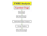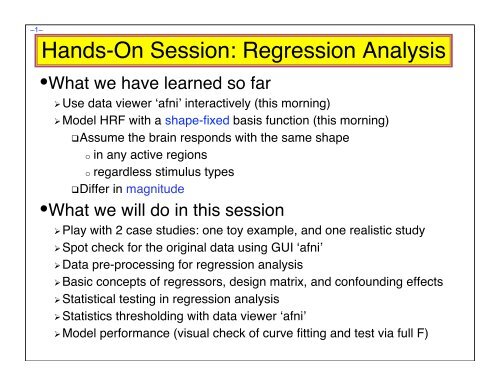
Hands-On Session: Regression Analysis

–5–• 3dvolreg outputScreen Output of the epi_r1_decon script++ 3dvolreg: AFNI version=AFNI_2007_05_29_1644 (Sep 5 2007) [64-bit]++ Reading input dataset ./epi_r1+orig.BRIK++ Edging: x=3 y=3 z=2++ Initializing alignment base++ Starting final pass on 67 sub-bricks: 0..1..2..3.. *** ..63..64..65..66..++ CPU time for realignment=5.35 s [=0.0799 s/sub-brick]++ Min : roll=-0.103 pitch=-1.594 yaw=-0.038 dS=-0.354 dL=-0.021 dP=-0.191++ Mean: roll=-0.047 pitch=+0.061 yaw=+0.023 dS=+0.006 dL=+0.032 dP=-0.076++ Max : roll=+0.065 pitch=+0.290 yaw=+0.055 dS=+0.050 dL=+0.120 dP=+0.113++ Max displacement in automask = 2.46 (mm) at sub-brick 42++ Wrote dataset to disk in ./epi_r1_reg+orig.BRIK• 3dDeconvolve output++3dDeconvolve: AFNI version=AFNI_2007_05_29_1644 (Sep 5 2007) [64-bit]++ Authored by: B. Douglas Ward, et al.++ loading dataset epi_r1_reg+orig*+ WARNING: Input polort=1; Longest run=201.0 s; Recommended minimum polort=2++ -stim_times using TR=3 seconds++ '-stim_times 1' using LOCAL times++ Wrote matrix image to file epi_r1_Xmat.jpg++ Wrote matrix values to file epi_r1_Xmat.x1D++ Signal+Baseline matrix condition [X] (64x3): 2.59165 ++ VERY GOOD ++++ Signal-only matrix condition [X] (64x1): 1 ++ VERY GOOD ++++ Baseline-only matrix condition [X] (64x2): 1.08449 ++ VERY GOOD ++++ -polort-only matrix condition [X] (64x2): 1.08449 ++ VERY GOOD ++++ Matrix inverse average error = 5.62791e-16 ++ VERY GOOD ++++ Calculations starting; elapsed time=0.238++ voxel loop:0123456789.0123456789.0123456789.0123456789.0123456789.++ Calculations finished; elapsed time=1.417++ Wrote bucket dataset into ./epi_r1_func+orig.BRIK++ Wrote 3D+time dataset into ./epi_r1_fitts+orig.BRIK++ #Flops=3.11955e+08 Average Dot Product=4.50251} Output file indicators} Maximum movement estimate} Output file indicators• If a program crashes, weʼll need to see this text output (at the very least)!} Consider '-polort 2'}Matrix QualityAssurance} Progress meter / pacifier

–6–Stimulus Timing: Input and Visualizationepi_r1_times.1D = 9.0 69.0 129.0= times of start of each BLOCK(30) HRF copyX matrixcolumns• HRF⊗timing• Linear in t• All onesaiv epi_r1_Xmat.jpg1dplot -sepscl epi_r1_Xmat.x1D

–7–Look at the Activation Map• Run afni to view what weʼve got (N.B.: a weak test with only 1 run) Switch Underlay to epi_r1_reg (background: input for 3dDeconvolve) Switch Overlay to epi_r1_func (statistics: output from 3dDeconvolve) Sagittal Image and Graph viewers (time series at a few voxels) FIM→Ignore→3 to have graph viewer not plot 1st 3 time pts FIM→Pick Ideal; pick epi_r1_ideal.1D (HRF: output from –x1D)• Define Overlay to set up functional coloring Olay→Allstim#0_Coef (sets coloring to be from β: color spectrum) Thr→Allstim#0_Tstat (sets threshold to be t-statistic: slider bar) See Overlay (otherwise wonʼt see the function!) – should be on automatically Play with threshold slider to get a meaningful activation map (e.g., t(61)=3is a decent threshold — more on thresholds later)Again, use Jump to (i j k) to jump to index coordinates 22 43 12

–8–Visually check model performance• Graph viewer: Opt→Tran 1D→Dataset #N to plot the modelfit dataset output by 3dDeconvolve• Will open the control panel for the Dataset #N plugin• Click first Input line to be ʻonʼ; then choose Datasetepi_r1_reg+orig• Also choose Color dk-blue to get a pleasing plot• Click 2nd Input on; then choose Dataset epi_r1_fitts+orig• Also choose Color limegreen to get a pleasing plot• Then click on Set+Close (to close the pluginʼs control panel)• This tool lets you visualize the quality of the data fit• Can also now overlay function on MP-RAGE anatomical byusing Switch Underlay to anat+orig dataset• Probably wonʼt want to graph the anat+orig dataset!

–9–More Realistic Study•The Experiment★ Cognitive Task: Subjects see photographs of two people interactingo The mode of communication falls in one of 3 categories: via telephone, email,or face-to-face.o The affect portrayed is either negative, positive, or neutral in nature.★ Experimental Design: 3x3 Factorial design, BLOCKED trialso Factor A: CATEGORY - (1) Telephone, (2) E-mail, (3) Face-to-Faceo Factor B: AFFECT - (1) Negative, (2) Positive, (3) Neutralo A random 30-second block of photographs for a task (ON), followed by a 30-second block of the control condition of scrambled photographs (OFF)...o Each run has 3 ON blocks, 3 OFF blocks. 9 runs in a scanning session.

–10–★Illustration of Stimulus ConditionsAFFECTNegative Positive NeutralTelephone“Your project is lame,just like you!”“You are the bestproject leader!”“You finished theproject.”CATEGORYE-mailFace-to-Face"Ugh, your hairis hideous!"“I curse the day I metyou!”"Your newhaircut looksawesome!"“I feel lucky to haveyou in my life.”"You got ahaircut."“I know who youare.”★Data Collectedo 1 Anatomical (MPRAGE) dataset for each subject➥ 124 axial slices➥ voxel dimensions = 0.938 x 0.938 x 1.2 mmo 9 Time Series (EPI) datasets for each subject➥ 34 axial slices x 67 volumes = 2278 slices per run➥ TR = 3 sec; voxel dimensions = 3.75 x 3.75 x 3.5 mmo Sample size, n=16 (all right handed)

–11–Multiple Stimulus Classes• Summary of the experiment 9 related communication stimulus types in a 3x3 design of Category byAffect (stimuli are shown to subject as pictures)o Telephone, Email & Face-to-face = categorieso Negative, Positive & Neutral = affects telephone stimuli: tneg, tpos, tneu email stimuli: eneg, epos, eneu face-to-face stimuli: fneg, fpos, fneu Each stimulus type has 3 presentation blocks of 30 s duration Scrambled pictures (baseline) are shown between blocks 9 imaging runs, 64 useful time points in eacho Originally, 67 TRs per run, but skip first 3 for MRI signal to reachsteady state (i.e., eliminate initial transient spike in data)o So 576 TRs of data, in total (64×9) Registered (3dvolreg) dataset: rall_vr+orig

–12–Regression with Multiple Model Files• Script file rall_decon does the job:• Run this script by typing tcsh rall_regress (takes a few minutes)3dDeconvolve -input rall_vr+orig \-jobs 2 \-concat '1D: 0 64 128 192 256 320 384 448 512' \-num_stimts 15 -local_times \-stim_times 1 '1D: 0 | | | 120 | | | | | 60' 'BLOCK(30)' \-stim_times 2 '1D: * | | 120 | | 0 | | | | 120' 'BLOCK(30)' \-stim_times 3 '1D: * | 120 | | 60 | | | | | 0' 'BLOCK(30)' \-stim_times 4 '1D: 60 | | | | | 120 | 0 | |' 'BLOCK(30)' \-stim_times 5 '1D: * | 60 | | 0 | | | 120 | |' 'BLOCK(30)' \-stim_times 6 '1D: * | | 0 | | 60 | | | 60 |' 'BLOCK(30)' \-stim_times 7 '1D: * | 0 | | | 120 | | 60 | |' 'BLOCK(30)' \-stim_times 8 '1D: 120 | | | | | 60 | | 0 |' 'BLOCK(30)' \-stim_times 9 '1D: * | | 60 | | | 0 | | 120 |' 'BLOCK(30)' \-stim_label 1 tneg -stim_label 2 tpos -stim_label 3 tneu \-stim_label 4 eneg -stim_label 5 epos -stim_label 6 eneu \-stim_label 7 fneg -stim_label 8 fpos -stim_label 9 fneu \• linear trend• try to use 2 CPUs• run start indexes• stimulus times• '|' indicates new run• response model• stimulus labelcontinued …

–13–Regression with Multiple Model Files (continued)-stim_file 10 motion.1D'[0]' -stim_base 10 \-stim_file 11 motion.1D'[1]' -stim_base 11 \-stim_file 12 motion.1D'[2]' -stim_base 12 \-stim_file 13 motion.1D'[3]' -stim_base 13 \-stim_file 14 motion.1D'[4]' -stim_base 14 \-stim_file 15 motion.1D'[5]' -stim_base 15 \-gltsym 'SYM: tpos -epos' -glt_label 1 TPvsEP \-gltsym 'SYM: tpos -tneg' -glt_label 2 TPvsTNg \-gltsym 'SYM: tpos tneu tneg -epos -eneu -eneg' \-glt_label 3 TvsE \-fout -tout \-bucket rall_func -fitts rall_fitts \-xjpeg rall_xmat.jpg -x1D rall_xmat.x1D• motion regressor• apply to baseline• symbolic GLT• label the GLT• statistic types to output• 9 visual stimulus classes were given using -stim_times• important to include motion parameters as regressors? this would remove the confounding effects due to motion artifacts 6 motion parameters as covariates via -stim_file and -stim_base motion.1D was generated from 3dvolreg with the -1Dfile option we can test the significance of the inclusion with –gltsymSwitch from -stim_base to -stim_label roll …Use -gltsym 'SYM: roll \ pitch \yaw \dS \dL \dP'

–14–Regressor Matrix for This Script (via -xjpeg)Baseline Visual stimuli Motion• 18 baseline regressors linear baseline 9 runs times 2 params• 9 visual stimulus regressors 3×3 design• 6 motion regressors 3 rotations and 3 shiftsaiv rall_xmat.jpg

–15–Regressor Matrix for This Script (via -x1D)baseline regressors: via 1dplot -sepscl xmat_rall.x1D'[0..17]'

–16–Regressor Matrix for This Script (via -x1D)• motion regressors• visual stimuli1dplot -sepscl xmat_rall.x1D'[18..$]'

–17–Options in 3dDeconvolve - 1-concat '1D: 0 64 128 192 256 320 384 448 512'• “File” that indicates where distinct imaging runs start inside the input file Numbers are the time indexes inside the dataset file for start of runs In this case, a text format .1D file put directly on the command lineo Could also be a filename, if you want to store that data externally-num_stimts 15 -local_times• We have 9 visual stimuli (+6 motion), so will need 9 -stim_times below• Times given in the -stim_times files are local to the start of each run (vs.-global_times meaning times are relative the start of the first run)-stim_times 1'1D: 0.0 | | | 120.0 | | | | | 60.0''BLOCK(30)'• “File” with 9 lines, each line specifying the start time in seconds for thestimuli within the corresponding imaging run, with the time measured relativeto the start of the imaging run itself (local time)

–18–Options in 3dDeconvolve - 2-gltsym 'SYM: tpos -epos' -glt_label 1 TPvsEP• GLTs are General Linear Tests• 3dDeconvolve provides test statistics for each regressor separately, but ifyou want to test combinations or contrasts of the β weights in each voxel,you need the -gltsym option• Example above tests the difference between the β weights for thePositive Telephone and the Positive Email responses Starting with SYM: means symbolic input is on command lineo Otherwise inputs will be read from a file Symbolic names for each regressor taken from -stim_label options Stimulus label can be preceded by + or - to indicate sign to use incombination of β weights Leave space after each label!• Goal is to test a linear combination of the β weights• Tests if β tpos = β epos• e.g., does tpos get different response from epos ?• Quiz: what would 'SYM: tpos epos fpos' test?It would test if βtpos+ βepos+ βfpos = 0

–19–Options in 3dDeconvolve - 3-gltsym 'SYM: tpos tneu tneg -epos -eneu -eneg'-glt_label 3 TvsE• Goal is to test if (β tpos+ β tneu+ β tneg)– (β epos + β eneu + β eneg ) = 0• Test average BOLD signal change among the 3 affects in the telephonetasks versus the email tasks-gltsym 'SYM: tpos –epos \ tneu –eneu \ tneg -eneg'-glt_label 3 TvsE_F• Goal is to test if β tpos= β epos, β tneu= β eneu, and β tneg= β enegare all true• BOLD signal change of any affect in the telephone tasks versus theemail tasks• This is a different test than the previous one!• -glt_label 3 TvsE option is used to attach a meaningful label to theresulting statistics sub-bricks• Output includes the ordered summation of the β weights and theassociated statistical parameters (t- and/or F-statistics)• t- or F-statistics?

–22–Statistics from 3dDeconvolve• An F-statistic measures significance of how much amodel component (stimulus class) reduced thevariance (sum of squares) of data time series residual After all the other model components were giventheir chance to reduce the variance Residuals ≡ data – model fit = errors = -errts A t-statistic sub-brick measures impact of onecoefficient (of course, BLOCK has only one coefficient)• Full F measures how much the all regressors ofinterest combined reduced the variance over just thebaseline regressors (sub-brick #0)• Individual partial-model F s measures how mucheach individual signal regressor reduced datavariance over the full model with that regressorexcluded (e.g., sub-bricks #3, #6, #9)• The Coef sub-bricks are the β weights (e.g., #1, #4,#7, #10) for the individual regressors• Also present: GLT coefficients and statisticsGroup Analysis: willbe carried out on β orGLT coefs from singlesubjectanalyses