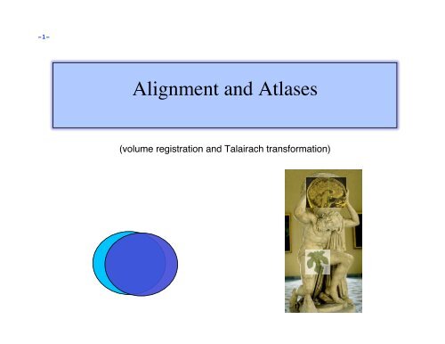
Alignment and Atlases

-4-Alignment tools in AFNI (continued)• align partial data to roughly the right part of the brain Nudge plug-in - visually align two volumes• rotate by known amount between volumes 3drotate – moves (shifts and rotates) volumes 3dWarp – make oblique, deoblique to match another dataset• Put centers of data from outside sources in roughly the same space @Align_Centers, 3dCM – put centers or centers of mass of dataset insame place• align specific regions across subjects 3dTagalign, tagset plugin – place and align volumes using correspondingfiducial marker points• align one jpeg image to another imreg – align two 2D images

-5-Image and Volume Registration with AFNI• Goal: bring images collected with different methods and at different times into spatialalignment• Facilitates comparison of data on a voxel-by-voxel basis Functional time series data will be less contaminated by artifacts due to subjectmovement Can compare results across scanning sessions once images are properly registered Can put volumes in standard space such as the stereotaxic Talairach-Tournouxcoordinates• Most (all?) image registration methods now in use do pair-wise alignment: Given a base image J(x) and target (or source) image I(x), find a geometricaltransformation T[x] so that I(T[x]) ≈ J(x)T[x] will depend on some parameters➥ Goal is to find the parameters that make the transformed I a ʻbest fitʼ to J To register an entire time series, each volume I n (x) is aligned to J(x) with its owntransformation T n [x], for n = 0, 1, …➥ Result is time series I n (T n [x]) for n=0, 1, …➥ User must choose base image J(x)

-6-• Most image registration methods make 3 algorithmic choices: How to measure mismatch E (for error) between I(T[x]) and J(x)?➥ Or … How to measure goodness of fit between I(T[x]) and J(x)?➭E(parameters) ≡ –Goodness(parameters) How to adjust parameters of T[x] to minimize E? How to interpolate I(T[x]) to the J(x) grid?➥ So can compare voxel intensities directly• The input volume is transformed by the optimal T[x] and a record of the transform is kept inthe header of the output. • Finding the transform to minimize E is the bulk of the registration work. Applying thetransform is easy and is done on the fly in many cases.• If data starts off far from each other, may add a coarse pass (twopass) step guess a lot among all the parameters (rotations, shifts, ...), measure cost best guesses, tweak the parameters(optimize) and measure againNow, applications of alignment…

-7-Within Modality Registration

-8-• AFNI program 3dvolreg is for aligning 3D volumes by rigid movements T[x] has 6 parameters:➥ Shifts along x-, y-, and z-axes; Rotations about x-, y-, and z-axes Generically useful for intra- and inter-session alignment Motions that occur within a single TR (2-3 s) cannot be corrected this way, sincemethod assumes rigid movement of the entire volume• AFNI program 3dWarpDrive is for aligning 3D volumes by affine transformations T[x] has up to 12 parameters:➥ Same as 3dvolreg plus 3 Scales and 3 Shears along x-, y-, and z-axes Generically useful for intra- and inter-session alignment Generically useful for intra- and inter-subject alignment• AFNI program 2dImReg is for aligning 2D slices T[x] has 3 parameters for each slice in volume:➥ Shift along x-, y-axes; Rotation about z-axis➥ No out of slice plane shifts or rotations! Useful for sagittal EPI scans where dominant subject movement is ʻnoddingʼ motionthat may be faster than TR It is possible and sometimes even useful to run 2dImReg to clean up sagittal noddingmotion, followed by 3dvolreg to deal with out-of-slice motion

-9-• Intra-session registration example: 3dvolreg -base 4 -heptic -zpad 4 \ -prefix fred1_epi_vr \ -1Dfile fred1_vr_dfile.1D \ fred1_epi+origInput dataset name -base 4 ⇒ Selects sub-brick #4 of dataset fred1_epi+orig as base image J(x) -heptic ⇒ Use 7 th order polynomial interpolation -zpad 4 ⇒ Pad each target image, I(x), with layers of zero voxels 4 deep on eachface prior to shift/rotation, then strip them off afterwards (before output)➥ Zero padding is particularly desirable for -Fourier interpolation➥ Is also good to use for polynomial methods, since if there are large rotations,some data may get ʻlostʼ when no zero padding if used (due to the 4-way shiftalgorithm used for very fast rotation of 3D volume data) -prefix fred1_epi_vr ⇒ Save output dataset into a new dataset with thegiven prefix name (e.g., fred1_epi_vr+orig) -1Dfile fred1_vr_dfile.1D ⇒ Save estimated movement parameters into a1D (i.e., text) file with the given name➥ Movement parameters can be plotted with command1dplot -volreg -dx 5 -xlabel Time fred1_vr_dfile.1D

-11-Motion correction – caveats• Motion is usually not completely correctable, so set motion parameters asregressors of no interest. Interpolation generally blurs data and depends onmethod and grid/resolution of EPI.• Check in the AFNI GUI to be sure the data is not bouncing around aftercorrection• Example – Monkey sips juice at stimulus time, and large jaw muscles move. Ifthe muscles are not masked, then motion correction may track muscles ratherthan brain. original 3dvolreg automask, 3dvolreg

-12-Cross Modality Registration

-13-align_epi_anat.py• Goal: Want to align anat and EPI (anat to EPI or EPI to anat or dset1to2 ordset2to1)LPC method – Local Pearson Correlation to match dark CSF in anatomical datawith bright CSF in EPI data.• align_epi_anat.py script – preprocessing and calls 3dAllineate for alignment• @AddEdge – for visualization• Simple Example:align_epi_anat.py -anat anat+orig \cd AddEdgeafni -niml -yesplugouts &@AddEdge-epi epi_r1+orig \-AddEdge -epi_base 0 -suffix _al4classCombines deoblique, motion correction, alignment and talairach transformationsinto a single transformation. Also performs slice timing correction and appliestransformations to “child” datasets.

-14-@Add@AddEdgedisplayBeforeAfter

-15-Alignment Visualization in AFNI• Graph and image – travel through time for motion correction or for a thousanddatasets in a row.• Multiple controllers and crosshairs – up to ten datasets at a time, quick andrough.• Overlay display – opacity control, thresholding. A single pair – good for differentor similar datasets.• Overlay toggle, Underlay toggle – wiggle, good but a little tricky• Checkerboard Underlay – two similar datasets in underlay but must be virtuallyidentical.• Edge display for underlay – effective pairwise comparison for quick finestructure display and comparison with overlay dataset with opacity. One datasetshould have reliable structure and contrast.• @AddEdge – single or dual edges with good contrast for pairwise comparison.

-16-Alignment strategies with align_epi_anat.py• Defaults work usually (>90% - FCON1000)• Problems: Far off start – “-giant_move”, “-big_move” Poor contrast – “-cost lpa”, “-cost nmi”, “-cost lpc+ZZ” Poor non-uniformity – “-edge”, “-cost lpa” stroke/MS lesions, tumors, monkeys, rats, something else? – see us, postmessage

-17-Rat BrainsAlignmentof12hourManganeseenhancedMRIscan(MEMRI)tostart#!/bin/tcsh# align_times.cshset basedset = 14_pre+origforeach timedset ( 14_*hr+orig.HEAD)align_epi_anat.py -prep_off -anat $timedset -epi $basedset \-epi_base 0 -anat_has_skull no -epi_strip None -suffix _edge2prep \-cost lpa -overwrite -edge -rat_alignend3dTcat -prefix 14_timealigned_edge 14_pre+orig. 14*edge2prep+orig.HEADDatafromDer‐YowChen,XinYu(NINDS)

-18-afni_proc.py – alignment handling • Single script to do all the processing of a typical fMRI pipeline including motioncorrection (3dvolreg), alignment (align_epi_anat.py)• combines transformations when possible• from example 6 in afni_proc.pyʼs prodigious help:afni_proc.py -subj_id sb23.e6.align \-dsets sb23/epi_r??+orig.HEAD \-do_block align tlrc \-copy_anat sb23/sb23_mpra+orig \-tcat_remove_first_trs 3 \-volreg_align_to last \-volreg_align_e2a \-volreg_tlrc_warp \…To process in orig space, remove -volreg_tlrc_warp.To apply manual tlrc transformation, use -volreg_tlrc_adwarp.To process as anat aligned to EPI, remove -volreg_align_e2a.

-19-ATLASES

-20-ATLAS DEFINITIONSTemplate - a reference dataset used for matching shapes.Examples: TT_N27+tlrc, MNI_EPI+tlrc, TT_ICBM452+tlrc.TT_N27+tlrc

-21-ATLAS DEFINITIONSTemplate Space - x,y,z coordinate system shared by manydatasets (the basic shoebox) Examples: TLRC (Talairach-Tourneaux), MNI, MNI_ANAT, ORIG.

-22-Atlas - segmentation info.ATLAS DEFINITIONSExamples: TTatlas+tlrc, TT_N27_EZ_ML+tlrc, roidset+orig.TT_N27_EZ_ML+tlrc

-23-Registration To Standard SpacesTransforming Datasets to Talairach-Tournoux Coordinates• The original purpose of AFNI (circa 1994 A.D.) was to perform the transformation ofdatasets to Talairach-Tournoux (stereotaxic) coordinates• The transformation can be manual, or automatic• In manual mode, you must mark various anatomical locations, defined in Jean Talairach and Pierre Tournoux “Co-Planar Stereotaxic Atlas of the Human Brain” Thieme Medical Publishers, New York, 1988 Marking is best done on a high-resolution T1-weighted structural MRI volume• In automatic mode, you need to choose a template to which your data arealigned. Different templates are made available with AFNIʼs distribution. You canalso use your own templates.• Transformation carries over to all other (follower) datasets in the same directory This is where the importance of getting the relative spatial placement of datasetsdone correctly in to3d really matters You can then write follower datasets, typically functional or EPI timeseries, to diskin Talairach coordinates➥ Purpose: voxel-wise comparison with other subjects➥ May want to blur volumes a little before comparisons, to allow for residualanatomic variability: AFNI programs 3dmerge or 3dBlurToFWHM

-24-Standard SpacesWhy use a standard template space?• Compare across subjects and groups easily for every voxel in the brain• Standardize coordinates with others• Know where a voxel is automatically from an atlas• Mostly automated and no specific ROI drawing requiredWhy not use a standard template space?• Inconsistency among subjects• Inconsistency among groups – elderly versus younger• Use consistent anatomical ROIs with good anatomical knowledge• Lower threshold for multiple comparison adjustments

-25-• Hidden in GUI - right click on “DataDir” or set AFNI_ENABLE_MARKERS toYES in .AFNIRC• Manual Transformation proceeds in two stages:1. Alignment of AC-PC and I-S axes (to +acpc coordinates)2. Scaling to Talairach-Tournoux Atlas brain size (to +tlrc coordinates)• Stage 1: Alignment to +acpc coordinates: Anterior commissure (AC) and posterior commissure (PC) are aligned to be they-axisThe longitudinal (inter-hemispheric or mid-sagittal) fissure is aligned to be the yzplane,thus defining the z-axisThe axis perpendicular to these is the x-axis (right-left)Five markers that you must place using the [Define Markers] control panel:AC superior edgeAC posterior marginPC inferior edgeFirst mid-sag point = top middle of anterior commissure = rear middle of anterior commissure = bottom middle of posterior commissure = some point in the mid-sagittal planeAnother mid-sag point = some other point in the mid-sagittal planeThis procedure tries to follow the Atlas as precisely as possible➥Even at the cost of confusion to the user (e.g., you)

-26-Click DefineMarkers toopen the“markers”panelPress this IN to create or change markersColor of“primary” (selected)markerColor of “secondary” (notselected) markersSize of markers (pixels)Size of gap in markersClear (unset)primary markerSelect whichmarker youare editingSet primary marker tocurrent focus locationCarry out transformationto +acpc coordinatesPerform “quality” check onmarkers (after all 5 are set)

-27-• Stage 2: Scaling to Talairach-Tournoux (+tlrc)coordinates: Once the AC-PC landmarks are set and we are in ACPC view, we nowstretch/shrink the brain to fit the Talairach-Tournoux Atlas brain size (sampleTT Atlas pages shown below, just for fun)Most anterior to AC70 mmAC to PC23 mmPC to most posterior79 mmLength of cerebrum172mmMost inferior to AC42 mmAC to most superior74 mmHeight of cerebrum116mmAC to left (or right)68 mmWidth of cerebrum136mm

-28-• Selecting the Talairach-Tournoux markers for the bounding box:There are 12 sub-regions to be scaled (3 A-P x 2 I-S x 2 L-R)To enable this, the transformed +acpc dataset gets its own set of markers➥ Click on the [AC-PC Aligned] button to view our volume in ac-pc coordinates➥Select the [Define Markers] control panelA new set of six Talairach markers will appear and the user now sets the bounding box markers(see Appendix C for details):Talairach markersappear only when theAC-PC view ishighlightedOnce all the markers are set, and the quality tests passed. Pressing [Transform Data] willwrite new header containing the Talairach transformations (see Appendix C for details) ➥ Recall: With AFNI, spatial transformations are stored in the header of the output

-29-Automatic Talairach Transformation with @auto_tlrc• Is manual selection of AC-PC and Talairach markers bringing you down? You can nowperform a TLRC transform automatically using an AFNI script called @auto_tlrc. Differences from Manual Transformation:➥ Instead of setting ac-pc landmarks and volume boundaries by hand, the anatomicalvolume is warped (using 12-parameter affine transform) to a template volume inTLRC space. ➥ Anterior Commisure (AC) center no longer at 0,0,0 and size of brain box is that ofthe template you use. ➭For various reasons, some good and some bad, templates adopted by theneuroimaging community are not all of the same size. Be mindful when usingvarious atlases or comparing standard-space coordinates.➥ You, the user, can choose from various templates for reference but be consistent inyour group analysis.➥ Easy, automatic. Just check final results to make sure nothing went seriously awry.AFNI is perfect but your data is not.

-30- Templates in @auto_tlrc that the user can choose from:➥ TT_N27+tlrc: ➭ AKA “Colin brain”. One subject (Colin) scanned 27 times and averaged.(www.loni.ucla.edu, www.bic.mni.mcgill.ca) ➭ Has a full set of FreeSurfer (surfer.nmr.mgh.harvard.edu) surface models thatcan be used in SUMA (link). ➭ Is the template for cytoarchitectonic atlases (www.fz-juelich.de/ime/spm_anatomy_toolbox)• For improved alignment with cytoarchitectonic atlases, I recommend using the TT_N27template because the atlases were created for it. In the future, we might provideatlases registered to other templates.➥ TT_icbm452+tlrc: ➭ International Consortium for Brain Mapping template, average volume of452 normal brains. (www.loni.ucla.edu, www.bic.mni.mcgill.ca)➥ TT_avg152T1+tlrc: ➭ Montreal Neurological Institute (www.bic.mni.mcgill.ca) template, averagevolume of 152 normal brains. ➥ TT_EPI+tlrc:➭ EPI template from spm2, masked as TT_avg152T1. TT_avg152 and TT_EPIvolumes are based on those in SPM's distribution. (www.fil.ion.ucl.ac.uk/spm/)

-31-Templates included with AFNITT_N27TT_avg152T1TT_avg152T2TT_ICBM452 TT_EPI MNI_avg152T2

-32-Steps performed by @auto_tlrc• For warping a volume to a template (Usage mode 1):1. Pad the input data set to avoid clipping errors from shifts androtations2. Strip skull (if needed) 3. Resample to resolution and size of TLRC template4. Perform 12-parameter affine registration using 3dWarpDrive Many more steps are performed in actuality, to fix up various pesky little artifacts. Read the script if you are interested.Typically this steps involves a high-res anatomical to an anatomicaltemplate ➥Example: @auto_tlrc -base TT_N27+tlrc. -input anat+orig. -suffix NONEOne could also warp an EPI volume to an EPI template.➥If you are using an EPI time series as input. You must choose onesub-brick to input. The script will make a copy of that sub-brick andwill create a warped version of that copy.

-33-Applying a transform to follower datasets• Say we have a collection of datasets that are in alignment with each other. Oneof these datasets is aligned to a template and the same transform is now to beapplied to the other follower datasets • For Talairach transforms there are a few methods: Method 1: Manually using the AFNI interface (see Appendix C) Method 2: With program adwarp➥adwarp -apar anat+tlrc -dpar func+origThe result will be: func+tlrc.HEAD and func+tlrc.BRIK Method 3: With @auto_tlrc script in mode 2➥ ONLY when -apar dataset was created by @auto_tlrc➥ @auto_tlrc -apar SubjectHighRes+tlrc. \➥➥-input Subject_EPI+orig. -dxyz 3(the output is named Subject_EPI_at+TLRC, by default)• Why bother saving transformed datasets to disk anyway? Datasets without .BRIK files are of limited use, only for display of slice images

-34-@auto_tlrc Example• Transforming the high-resolution anatomical: (If you are also trying the manual transform on workshop data, startwith a fresh directory with no +tlrc datasets )@auto_tlrc \-base TT_N27+tlrc \-suffix NONE \-input anat+orig• Transforming the function (“follower datasets”), setting the resolution at 2mm:@auto_tlrc \ -apar anat+tlrc \ -input func_slim+orig \ -suffix NONE \ -dxyz 2 Output:anat+tlrcOutput:func_slim+tlrc • You could also use the icbm452 or the mniʼs avg152T1 template insteadof N27 or any other template you like (see @auto_tlrc -help for a fewgood words on templates)

-35-@auto_tlrc Results are Comparable to Manual TLRC:@auto_tlrcOriginalManual

-36-Comparing data • How can I compare regions/voxels across subjects and groups? What works “best”? @auto_tlrc – affine registration method to align individual subjects to atemplate – useful for most applications. manual Talairach – based on specific markers divides data up basedon AC-PC line and brain enclosing boxes. Better for looking at medialstructures. 3dTagalign – place markers on specific corresponding points amongdatasets and align with affine transformation ROI creation – draw ROIʼs (Draw Dataset plug-in) for each structure

-37-Atlas/Template Spaces Differ In SizeMNI is larger than TLRC space.

-38-Atlas/Template Spaces Differ In OriginTLRCMNIMNI-Anat.

-39-From Space To SpaceTLRCMNIMNI-Anat.• Going between TLRC and MNI: Approximate equation➥used by whereami and 3dWarp Manual TLRC transformation of MNI template to TLRC space ➥ used by whereami (as precursor to MNI Anat.), based on N27 template Automated registration of a any dataset from one space to the other• Going between MNI and MNI Anatomical (Eickhoff et al. Neuroimage 25, 2005): MNI + ( 0, 4, 5 ) = MNI Anat. (in RAI coordinate system) • Going between TLRC and MNI Anatomical (as practiced in whereami): Go from TLRC to MNI via manual xform of N27 template Add ( 0, 4, 5 )

-40-Atlases/Templates Use Different Coord. Systems• There are 48 manners to specify XYZ coordinates• Two most common are RAI/DICOM and LPI/SPM• RAI means X is Right-to-Left (from negative-to-positive) Y is Anterior-to-Posterior (from negative-to-positive) Z is Inferior-to-Superior• LPI means(from negative-to-positive) X is Left-to-Right (from negative-to-positive) Y is Posterior-to-Inferior (from negative-to-positive) Z is Inferior-to-Superior (from negative-to-positive)• To go from RAI to LPI just flip the sign of the X and Y coordinates Voxel -12, 24, 16 in RAI is the same as 12, -24, 16 in LPI Voxel above would be in the Right, Posterior, Superior octant of the brain• AFNI allows for all coordinate systems but default is RAI Can use environment variable AFNI_ORIENT to change the default forAFNI AND other programs. See whereami -help for more details.

-41-Atlases Distributed With AFNITT_Daemon• TT_Daemon : Created by tracing Talairach and Tournoux brain illustrations. Generously contributed by Jack Lancaster and Peter Fox of RIC UTHSCSA)

-42-Atlases Distributed With AFNIAnatomy Toolbox: Prob. Maps, Max. Prob. Maps• CA_N27_MPM, CA_N27_ML, CA_N27_PM: Anatomy Toolbox's atlases withsome created from cytoarchitectonic studies of 10 human post-mortem brains Generously contributed by Simon Eickhoff, Katrin Amunts and Karl Zilles ofIME, Julich, Germany

-43-Atlases Distributed With AFNI:Anatomy Toolbox: MacroLabels• CA_N27_MPM, CA_N27_ML, CA_N27_PM: Anatomy Toolbox's atlases withsome created from cytoarchitectonic studies of 10 human post-mortem brains Generously contributed by Simon Eickhoff, Katrin Amunts and Karl Zilles ofIME, Julich, Germany

-44-• Some fun and useful things to do with +tlrc datasets are on the 2D slice viewerButton-3 pop-up menu:[Talairach to]Lets you jump to centroid of regions in the TT_Daemon Atlas (works in +orig too)

-45-[Where am I?]Shows you where youare in various atlases. (works in +orig too, ifyou have a TTtransformed parent)For atlas installation,and much much more,see help in commandline version:whereami -help

-46-• whereami can provide the user with more detailed informationregarding the output of 3dclust– For instance, say you want more information regarding the center of mass voxelsfrom each cluster (from the 3dclust output). I.e., where do they fall approximatelywithin the atlases?3dclust -dxyz=1 -1clip 9.5 1 1000 func_FullF+tlrc > clusts.1Dwhereami -coord_file clusts.1D'[1,2,3]' -tab | lessCenter of mass output,columns 1,2,3, from 3dclustoutput (see pg. 25).Shown: Cluster#1’s coordinatesaccording tovarious atlases(TT, MNI, etc), aswell as the nameof the anatomicalstructure that islocated at or nearthese coordinates(which may varyby atlas)etc…

-47-• whereami can report on the overlap of ROIs with atlasdefinedregionswhereami -omask anat_roi+tlrc

-48-[Atlas colors]Lets you display color overlays for various TT_Daemon Atlas-defined regions,using the Define Function See TT_Daemon Atlas Regions control (works only in+tlrc)For the moment, atlas colors work for TT_Daemon atlas only. There are ways todisplay other atlases. See whereami -help.

-49-The Future …• New atlases – easy and fun. Make your own! make available in AFNI GUI and whereami and to other users• New templates and template spaces – fully supported in AFNI macaque rat, mouse, human pediatric, …• On-the-fly transformations through all available template spaces• Extra information about atlas structures

-50-Individual SubjectsFreeSurfersegmentationManualsegmentationOverlay panel shows structure name.Soon also from whereami.

-51-Neighborhoods in Space -Transformation ChainsTx1_3groupmeanS1S3Tx3_4pediatrictemplateorigTx4_6Tx1_2S4S6S2tlrcTx2_5S5Tx4_5mni anatExample spacetransformation chains:S1->S5 = Tx1_2,Tx2_5S6->S2 =Tx4_6,Tx4_5,Tx2_5mni

-52-Questions, comments, concerns, suggestions, lunch?Charles Atlas

-53-• Histogram cartoons:IIIJJJ• J not useful inpredicting I• I can be accuratelypredicted from J witha linear formula:-leastsq is OK• I can be accuratelypredicted from J, butnonlinearly:-leastsq is BAD

-54-• Actual histograms from a registration example J(x) = 3dSkullStrip-ed MPRAGE I(x) = EPI volumeIIJJ• Before alignment• After alignment(using -mutualinfo)

-55-• grayscale underlay = J(x) = 3dSkullStrip-ed MPRAGE• color overlay = I(x) = EPI volume• Before alignment• After alignment(using -mutualinfo)

-56-• Other 3dAllineate capabilities: Save transformation parameters with option -1Dfile in one program run➥ Re-use them in a second program run on another input dataset with option-1Dapply Interpolation: linear (polynomial order = 1) during alignment➥ To produce output dataset: polynomials of order 1, 3, or 5• Algorithm details: Initial alignment starting with many sets of transformation parameters, using onlya limited number of points from smoothed images The best (smallest E) sets of parameters are further refined using more pointsfrom the images and less blurring This continues until the final stage, where many points from the images and noblurring is used• So why not 3dAllineate all the time? Alignment with cross-modal cost functions do not always converge as well asthose based on least squares. ➥ See Appendix B for more info.➥ Improvements are still being introduced

-57-• The future for 3dAllineate: Allow alignment to use manually placed control points (on both images) and theimage data➥ Will be useful for aligning highly distorted images or images with severe shading➥ Current AFNI program 3dTagalign allows registration with control points only Nonlinear spatial transformations➥ For correcting distortions of EPI (relative to MPRAGE or SPGR) due to magneticfield inhomogeneity ➥ For improving inter-subject brain alignment (Talairach) Investigate the use of local computations of E (in a set of overlapping regions coveringthe images) and using the sum of these local Eʼs as the cost function➥ May be useful when relationship between I and J image intensities is spatiallydependent➭ RF shading and/or Differing MRI contrasts Save warp parameters in dataset headers for re-use by 3dWarp

-58-Detailed example for manual transformation is now in appendix C• Listen up folks, IMPORTANT NOTE:Have you ever opened up the [Define Markers] panel, only to find the AC-PC markersmissing , like this:Gasp! Wheredid they go? There are a few reasons why this happens, but usually itʼs because youʼve made a copyof a dataset, and the AC-PC marker tags werenʼt created in the copy, resulting in theabove dilemma.➥ In other cases, this occurs when afni is launched without any datasets in thedirectory from which it was launched (oopsy, your mistake). If you do indeed have an AFNI dataset in your directory, but the markers are missingand you want them back, run 3drefit with the -markers options to create an emptyset of AC-PC markers. Problem solved!3drefit -markers

-59-Appendix AInter-subject, inter-session registration

-60-• Intra-subject, inter-session registration (for multi-day studies on same subject) Longitudinal or learning studies; re-use of cortical surface models Transformation between sessions is calculated by registering high-resolutionanatomicals from each session➥ to3d defines definesrelationship between EPIand SPGR in each session➥ 3dvolreg computesrelationship betweensessions➥ So can transform EPI fromsession 2 to orientation ofsession 1 Issues in inter-session registration:➥ Subjectʼs head will be positioned differently (in orientation and location)➭ xyz-coordinates and anatomy donʼt correspond➥ Anatomical coverage of EPI slices will differ between sessions➥ Geometrical relation between EPI and SPGR differs between session➥ Slice thickness may vary between sessions (try not to do this, OK?)

-61-• Anatomical coverage differs At acquisition:Day 2 is rotatedrelative to Day 1 After rotation tosame orientation,then clipping toDay 2 xyz-grid

-62- Another problem: rotationoccurs around center ofindividual datasets

-63- Solutions to these problems:➥ Add appropriate shift to E2 on top of rotation➭ Allow for xyz shifts between days (E1-E2), and center shiftsbetween EPI and SPGR (E1-S1 and E2-S2)➥ Pad EPI datasets with extra slices of zeros so that aligned datasetscan fully contain all data from all sessions➥ Zero padding of a dataset can be done in to3d (at dataset creationtime), or later using 3dZeropad➥ 3dvolreg and 3drotate can zero pad to make the output match a“grid parent” dataset in size and location

-64-Recipe for intra-subject S2-to-S1 transformation:1. Compute S2-to-S1 transformation:3dvolreg -twopass -zpad 4 -base S1+orig \ • -twopass allows -prefix S2reg S2+origfor larger motions➥ Rotation/shift parameters are saved in S2reg+orig.HEAD2. If not done before (e.g., in to3d), zero pad E1 datasets:3dZeropad -z 4 -prefix E1pad E1+orig3. Register E1 datasets within the session:3dvolreg -base ‘E1pad+orig[4]’ -prefix E1reg \ E1pad+orig4. Register E2 datasets within the session, at the same time executinglarger rotation/shift to session 1 coordinates that were saved in S2reg+orig.HEAD:➥➥3dvolreg -base ‘E2+orig[4]’ \ -rotparent S2reg+orig \ • These options put the aligned -gridparent E1reg+orig \ • E2reg into the same coordinates -prefix E2reg E2reg+orig and grid as E1reg-rotparent tells where the inter-session transformation comes from-gridparent defines the output grid location/size of new dataset➭ Output dataset will be shifted and zero padded as needed to lie ontop of E1reg+orig

-65- Recipe above does not address problem of having different slice thickness indatasets of the same type (EPI and/or SPGR) in different sessions➥ Best solution: pay attention when you are scanning, and always use thesame slice thickness for the same type of image➥ OK solution: use 3dZregrid to linearly interpolate datasets to a new slicethickness Recipe above does not address issues of slice-dependent time offsets storedin data header from to3d (e.g., ʻalt+zʼ)➥ After interpolation to a rotated grid, voxel values can no longer be said tocome from a particular time offset, since data from different slices will havebeen combined➥ Before doing this spatial interpolation, it makes sense to time-shift datasetto a common temporal origin➥ Time shifting can be done with program 3dTshift➭ Or by using the -tshift option in 3dvolreg, which first does thetime shift to a common temporal origin, then does the 3D spatialregistration• Further reading at the AFNI web site File README.registration (plain text) has more detailed instructions andexplanations about usage of 3dvolreg File regnotes.pdf has some background information on issues and methodsused in FMRI registration packages

-66-Appendix B3dAllineate for the curious

-67-

-68-Algorithmic Features• Uses Powellʼs NEWUOA software for minimization of general cost function• Lengthy search for initial transform parameters if two passes of registration are turnedon [which is the default] Random and grid search through hundreds of parameter sets for 15 good (low cost)parameter sets Optimize a little bit from each ʻgoodʼ set, using blurred images➥ Blurring the images means that small details wonʼt prevent a match Keep best 4 of these parameter sets, and optimize them some more [keeping 4 setsis the default for -twobest option]➥ Amount of blurring is reduced in several stages, followed by re-optimization ofthe transformation parameter sets on these less blurred images➥ -twofirst does this for first sub-brick, then uses the best parameter setsfrom the first sub-brick as the starting point for the rest of the sub-bricks [thedefault] Use best 1 of these parameter sets as starting point for fine (un-blurred) parameteroptimization➥ The slowest part of the program

-69-Algorithmic Features• Goal is to find parameter set w such that E[ J(x) , I(T(x,w)) ] is small T(x,w) = spatial transformation of x given w J() = base image, I() = target image, E[ ] = cost function• For each x in base image space, compute T(x,w) and then interpolate I() at thosepoints For speed, program doesnʼt use all points in J(), just a scattered collection ofthem, selected from an automatically generated mask➥ Mask can be turned off with -noauto option➥ At early stages, only a small collection of points [default=23456] is used whencomputing E[ ]➥ At later stages, more points are used, for higher accuracy➭ Recall that each stage is less blurred than the previous stages Large fraction of CPU time is spent in interpolation of image I() over the collectionof points used to compute E[ ]

-70-Cost Functions• Except for least squares (actually, ls minimizes E = 1.0 – Pearson correlation coefficient), allcost functions are computed from 2D joint histogram of J(x) and I(T(x,w)) Start and final histograms can be saved using hidden option -savehistBeforeAfterSourceimageSource image= rotated copyof Base imageBase image

-72-Mutual Information• Entropy of 2D histogram H({r ij }) = –Σ ij r ij log 2 (r ij ) Number of bits needed to encode value pairs (i,j)• Mutual Information between two distributions Marginal (1D) histograms {p i } and {q j } MI = H({p i }) + H({q j }) - H({r ij }) Number of bits required to encode 2 values separately minus number of bitsrequired to encode them together (as a pair) If 2D histogram is independent (r ij = p i ⋅q j ) then MI = 0 = no gain from joint encoding• 3dAllineate minimizes E[J,I] = –MI(J,I) with -cost mi

-73-Normalized MI• NMI = H({r ij }) ⁄ [ H({p i }) + H({q j }) ] Ratio of number of bits to encode value pair divided by number of bits to encode twovalues separately Minimize NMI with -cost nmi• Some say NMI is more robust for registration than MI, since MI can be large when thereis no overlap between the two images NOoverlapBADoverlap100%overlap

-74-Hellinger Metric• MI can be thought of as measuring a ʻdistanceʼ between two 2D histograms: thejoint distribution {r ij } and the product distribution {p i ⋅q j } MI is not a ʻtrueʼ distance: it doesnʼt satisfy triangle inequality d(a,b)+d(b,c) >d(a,c)• Hellinger metric is a true distance in distribution “space”: HM = Σ ij [ √r ij – √(p i ⋅q j ) ] 2 3dAllineate minimizes –HM with -cost hel This is the default cost functionbca

-75-Correlation Ratio• Given 2 (non-independent) random variables x and y Exp[y|x] is the expected value (mean) of y for a fixedvalue of x➥ Exp[a|b] ≡ Average value of ʻaʼ, given value of ʻbʼ Var(y|x) is the variance of y when x is fixed = amountof uncertainty about value of y when we know x➥ v(x) ≡ Var(y|x) is a function of x onlyxy• CR(x,y) ≡ 1 – Exp[v(x)] ⁄ Var(y) • Relative reduction in uncertainty about value of y when x is known; large CR meansExp[y|x] is a good prediction of the value of y given the value of x• Does not say that Exp[x|y] is a good prediction of the x given y• CR(x,y) is a generalization of the Pearson correlation coefficient, which assumes thatExp[y|x] = α⋅x+β

-76-3dAllineateʼs Symmetrical CR• First attempt to use CR in 3dAllineate didnʼt give good results• Note asymmetry: CR(x,y) ≠ CR(y,x)• 3dAllineate now offers two different symmetric CR cost functions: Compute both unsymmetric CR(x,y) and CR(y,x), then combine byMultiplying or Adding: CRm(x,y) = 1 – [ Exp(v(x))⋅Exp(v(y)) ] ⁄[ Var(y) ⋅ Var(x) ] = CR(x,y) + CR(y,x) – CR(x,y) ⋅ CR(y,x) CRa(x,y) = 1 – 1 / 2 [ Exp(v(x)) ⁄ Var(y) ] – 1 / 2 [Exp(v(y)) ⁄= [ CR(x,y) + CR(y,x) ] ⁄ 2Var(x) ] These work better than CR(J,I) in my test problems• If Exp[y|x] can be used to predict y and/or Exp[x|y] can be used to predict x,then crM(x,y) will be large (close to 1)• 3dAllineate minimizes 1 – CRm(J,I) with option -cost crM• 3dAllineate minimizes 1 – CRa(J,I) with option -cost crA• 3dAllineate minimizes 1 – CR(J,I) with option -cost crU

-77-Test: Monkey EPI - Anat6 DOFCRm6 DOFNMI

-78-Test: Monkey EPI - Anat6 DOFHEL6 DOFMI

-79-Test: Monkey EPI - Anat11 DOFCRm11 DOFNMI

-80-Test: Monkey EPI - Anat11 DOFHEL11 DOFMI

-81-Appendix CTalairach Transform from the days of yore

-82-• Listen up folks, IMPORTANT NOTE:Have you ever opened up the [Define Markers] panel, only to find the AC-PC markersmissing , like this:Gasp! Wheredid they go? There are a few reasons why this happens, but usually itʼs because youʼve made a copyof a dataset, and the AC-PC marker tags werenʼt created in the copy, resulting in theabove dilemma.➥ In other cases, this occurs when afni is launched without any datasets in thedirectory from which it was launched (oopsy, your mistake). If you do indeed have an AFNI dataset in your directory, but the markers are missingand you want them back, run 3drefit with the -markers options to create an emptyset of AC-PC markers. Problem solved!3drefit -markers

-83-• Class Example - Selecting the ac-pc markers: cd AFNI_data1/demo_tlrc ⇒ Descend into the demo_tlrc/ subdirectory afni & ⇒ This command launches the AFNI program➥ The “&” keeps the UNIX shell available in the background, so we can continuetyping in commands as needed, even if AFNI is running in the foreground Select dataset anat+orig from the [Switch Underlay] control panelPress IN to viewmarkers on brainvolumeThe AC-PCmarkersappear onlywhen the origview ishighlighted Select the [Define Markers]control panel to view the 5 markers forac-pc alignment Click the [See Markers] button to view the markers on the brainvolume as you select them Click the [Allow edits] button in the ac-pc GUI to begin markerselection

-84- First goal is to mark top middle and rear middle of AC➥ Sagittal: look for AC at bottom level of corpus callosum, below fornix➥ Coronal: look for “mustache”; Axial: look for inter-hemispheric connection➥ Get AC centered at focus of crosshairs (in Axial and Coronal)➥ Move superior until AC disappears in Axial view; then inferior 1 pixel➥ Press IN [AC superior edge] marker toggle, then [Set]➥ Move focus back to middle of AC➥ Move posterior until AC disappears in Coronal view; then anterior 1 pixel➥ Press IN [AC posterior margin], then [Set]

-85- Second goal is to mark inferior edge of PC➥ This is harder, since PC doesnʼt show up well at 1 mm resolution➥ Fortunately, PC is always at the top of the cerebral aqueduct, which does showup well (at least, if CSF is properly suppressed by the MRI pulse sequence)cerebral aqueduct➥ Therefore, if you canʼt see the PC, find mid-sagittal location just at topof cerebral aqueduct and mark it as [PC inferior edge] Third goal is to mark two inter-hemispheric points (above corpuscallosum)➥ The two points must be at least 2 cm apart➥ The two planes AC-PC-#1 and AC-PC-#2 must be no more than 2 oapart

-86-• AC-PC Markers Cheat Sheet The AC-PC markers may take some time for the novice to master, so in the interest oftime, we provide you with a little guide or “cheat sheet” to help you place markers on thisexample volume: i j k to: AC Superior Edge: 126 107 63AC Posterior Margin:127 108 63 PC Inferior Edge: 152 109 63 1st Mid-Sagittal Point: 110 59 60 2nd Mid-Sagittal Point: 172 63 60AC-PCmarkersmid-sagittalmarkers

-87- Once all 5 markers have been set, the [Quality?] Button is ready➥ You canʼt [Transform Data] until [Quality?] Check is passed➥ In this case, quality check makes sure two planes from AC-PC line to midsagittalpoints are within 2 o➭ Sample below shows a 2.43 o deviation between planes ⇒ ERRORmessage indicates we must move one of the points a little➭ Sample below shows a deviation between planes at less than 2 o . Qualitycheck is passed• We can now save the marker locations into the dataset header

-88-Notes on positioning AC/PC markers:➥➥The structures dimensions are on the order of typical high-res images. Do not fret about amatter such as: ➭ Q: Do I put the Sup. AC marker on the top voxel where I see still the the structure or onthe one above it?• A: Either option is OK, just be consistent. The same goes for setting the boundingbox around the brain discussed ahead. Remember, intra-subject anatomicalvariability is more than the 1 or 2 mm you are concerned about.Typically, all three markers fall in the same mid-saggital planeWhy, oh why, two mid-saggital points?➥➥[Quality?] Contrary to our desires, no two hemispheres in their natural setting can beperfectly separated by a mid-saggital plane. When you select a mid-saggital point, you aredefining a plane (with AC/PC points) that forms an acceptable separation between left andright sides of the brain. To get a better approximation of the mid-saggital plane, AFNI insists on another midsaggitalpoint and uses the average of the two planes. It also insists that these two planesare not off from one another by more than 2 o I am Quality! How do I escape the tyranny of the [Quality?] check?➥ If you know what you're doing and want to elide the tests:➭➭Set AFNI_MARKERS_NOQUAL environment variable to YES This is a times needed when you are applying the transform to brains of children ormonkeys which differ markedly in size from mature human brains.

-89- When [Transform Data] is available, pressing it will close the[Define Markers] panel, write marker locations into the dataset header, andcreate the +acpc datasets that follow from this one➥ The [AC-PC Aligned] coordinate system is now enabled in the mainAFNI controller window➥ In the future, you could re-edit the markers, if desired, then re-transform thedataset (but you wouldnʼt make a mistake, would you?)➥ If you donʼt want to save edited markers to the dataset header, you mustquit AFNI without pressing [Transform Data] or [Define Markers] ls ⇒ The newly created ac-pc dataset, anat+acpc.HEAD, is located in ourdemo_tlrc/ directory At this point, only the header file exists, which can be viewed when selectingthe [AC-PC Aligned] button ➥ more on how to create the accompanying .BRIK file later…

-90-• Scaling to Talairach-Tournoux (+tlrc) coordinates: We now stretch/shrink the brain to fit the Talairach-Tournoux Atlasbrain size (sample TT Atlas pages shown below, just for fun)Most anterior to ACAC to PCPC to most posteriorMost inferior to ACAC to most superiorAC to left (or right)70 mm23 mm79 mm42 mm74 mm68 mmLength of cerebrum 172mmHeight of cerebrum116 mmWidth of cerebrum 136mm

-91-• Class example - Selecting the Talairach-Tournoux markers: There are 12 sub-regions to be scaled (3 A-P x 2 I-S x 2 L-R) To enable this, the transformed +acpc dataset gets its own set of markers➥ Click on the [AC-PC Aligned] button to view our volume in ac-pc coordinates➥ Select the [Define Markers] control panel A new set of six Talairach markers will appear:The Talairach markers appear onlywhen the AC-PC view is highlighted

-92-Using the same methods as before (i.e., select marker toggle, move focus there, [Set]),you must mark these extreme points of the cerebrum➥ Using 2 or 3 image windows at a time is useful➥ Hardest marker to select is [Most inferior point] in the temporal lobe, since itis near other (non-brain) tissue:Sagittal view:most inferiorpointAxial view:most inferiorpoint➥ Once all 6 are set, press [Quality?] to see if the distances are reasonable➭ Leave [Big Talairach Box?] Pressed IN➭ Is a legacy from earliest (1994-6) days of AFNI, when 3D box size of +tlrcdatasets was 10 mm smaller in I-direction than the current default

-93- Once the quality check is passed, click on [Transform Data] to save the+tlrc header ls ⇒ The newly created +tlrc dataset, anat+tlrc.HEAD, is located in ourdemo_tlrc/ directory➥ At this point, the following anatomical datasets should be found in ourdemo_tlrc/ directory:anat+orig.HEAD anat+orig.BRIKanat+acpc.HEADanat+tlrc.HEAD➥ In addition, the following functional dataset (which I -- the instructor --created earlier) should be stored in the demo_tlrc/ directory:func_slim+orig.HEADfunc_slim+orig.BRIK➭ Note that this functional dataset is in the +orig format (not +acpc or+tlrc)

-94-• Automatic creation of “follower datasets”: After the anatomical +orig dataset in a directory is resampled to +acpc and+tlrc coordinates, all the other datasets in that directory will automatically gettransformed datasets as well➥➥These datasets are created automatically inside the interactive AFNI program,and are not written (saved) to disk (i.e., only header info exists at this point)How followers are created (arrows show geometrical relationships): anat+orig → anat+acpc → anat+tlrc ↑ ↓ ↓ func+orig func+acpc func+tlrc

-95- How does AFNI actually create these follower datsets?➥ After [Transform Data] creates anat+acpc, other datasets in the samedirectory are scanned➭ AFNI defines the geometrical transformation (“warp”) from func_slim+origusing the to3d-defined relationship between func_slim+orig and anat+orig, AND the markers-defined relationship between anat+orig and anat+acpc • A similar process applies for warping func_slim+tlrc➭ These warped functional datasets can be viewed in the AFNI interface:Functional dataset warped toanat underlay coordinatesfunc_slim+orig “func_slim+acpc” “func_slim+tlrc” Next time you run AFNI, the followers will automatically be created internally againwhen the program starts

-96-“Warp on demand” viewing of datasets:➥ AFNI doesnʼt actually resample all follower datasets to a grid in the re-aligned and restretchedcoordinates➭ This could take quite a long time if there are a lot of big 3D+time datasets➥ Instead, the dataset slices are transformed (or warped) from +orig to +acpc or +tlrc forviewing as needed (on demand)➥ This can be controlled from the [Define Datamode] control panel:If possible, lets you view slices direct from dataset .BRIKIf possible, transforms slices from ‘parent’ directoryInterpolation mode used when transforming datasetsGrid spacing to interpolate withSimilar for functional datasetsWrite transformed datasets to diskRe-read: datasets from current session, all session, or 1D filesRead new: session directory, 1D file, dataset from Web addressMenus that had to go somewhereAFNI titlebar shows warp on demand:{warp}[A]AFNI2.56b:AFNI_sample_05/afni/anat+tlrc

-97-Creating follower data• Writing “follower datasets” to disk: Recall that when we created anat+acpc and anat+tlrc datasets by pressing[Transform Data], only .HEAD files were written to disk for them In addition, our follower datasets func_slim+acpc and func_slim+tlrc arenot stored in our demo_tlrc/ directory. Currently, they can only be viewed inthe AFNI graphical interface Questions to ask:1. How do we write our anat .BRIK files to disk?2. How do we write our warped follower datasets to disk? To write a dataset to disk (whether it be an anat .BRIK file or a follower dataset),use one of the [Define Datamode] ⇒ Resamp buttons:ULay writes current underlay dataset to diskOLay writes current overlay dataset to diskMany writes multiple datasets in a directory todisk

-98-• Class example - Writing anat (Underlay) datasets to disk: You can use [Define Datamode] ⇒ Write ⇒ [ULay] to write the currentanatomical dataset .BRIK out at the current grid spacing (cubical voxels), usingthe current anatomical interpolation mode After that, [View ULay Data Brick] will become available➥ ls ⇒ to view newly created .BRIK files in the demo_tlrc/ directory:anat+acpc.HEAD anat+acpc.BRIKanat+tlrc.HEAD anat+tlrc.BRIK• Class example - Writing func (Overlay) datasets to disk: You can use [Define Datamode] ⇒ Write ⇒ [OLay] to write the currentfunctional dataset .HEAD and BRIK files into our demo_tlrc/ directory After that, [View OLay Data Brick] will become available➥ ls ⇒ to view newly resampled func files in our demo_tlrc/ directory:func_slim+acpc.HEADfunc_slim+acpc.BRIKfunc_slim+tlrc.HEADfunc_slim+tlrc.BRIK

-99-• Command line program adwarp can also be used to write out .BRIK files fortransformed datasets:adwarp -apar anat+tlrc -dpar func+orig The result will be: func+tlrc.HEAD and func+tlrc.BRIK• Why bother saving transformed datasets to disk anyway? Datasets without .BRIK files are of limited use:➥ You canʼt display 2D slice images from such a dataset➥ You canʼt use such datasets to graph time series, do volume rendering,compute statistics, run any command line analysis program, run anyplugin…➭ If you plan on doing any of the above to a dataset, itʼs best to haveboth a .HEAD and .BRIK files for that dataset

-100- Examination of time series fred2_epi+orig and fred2_epi_vr_+origshows that head movement up and down happened within about 1 TRinterval➥ Assumption of rigid motion of 3D volumes is not good for this case fred1_epi registeredwith 2dImRegfred1_epi registeredwith 3dvolregfred1_epi unregistered➥ Can do 2D slice-wise registration with command2dImReg -input fred2_epi+orig \ -basefile fred1_epi+orig \ -base 4 -prefix fred2_epi_2Dreg Graphs of a single voxel time series nearthe edge of the brain:➥ Top = slice-wise alignment➥ Middle = volume-wise adjustment➥ Bottom = no alignment For this example, 2dImReg appears toproduce better results. This is becausemost of the motion is ʻhead noddingʼ andthe acquisition is sagittal You should also use AFNI to scroll throughthe images (using the Index control)during the period of pronounced movement Helps see if registration fixed problems

-101-No longer discussed here, see appendix A if interested• Intra-subject, inter-session registration (for multi-day studies on same subject) Longitudinal or learning studies; re-use of cortical surface models Transformation between sessions is calculated by registering high-resolutionanatomicals from each session➥ to3d defines definesrelationship between EPIand SPGR in each session➥ 3dvolreg computesrelationship betweensessions➥ So can transform EPI fromsession 2 to orientation ofsession 1 Issues in inter-session registration:➥ Subjectʼs head will be positioned differently (in orientation and location)➭ xyz-coordinates and anatomy donʼt correspond➥ Anatomical coverage of EPI slices will differ between sessions➥ Geometrical relation between EPI and SPGR differs between session➥ Slice thickness may vary between sessions (try not to do this, OK?)

-102-Real-Time 3D Image Registration• The image alignment method using in 3dvolreg is also built into theAFNI real-time image acquisition plugin Invoke by command afni -rt Then use Define Datamode → Plugins → RT Options to control the operation of real-time (RT) image acquisition• Images (2D or 3D arrays of numbers) can be sent into AFNI through aTCP/IP socket See the program rtfeedme.c for sample of how to connect toAFNI and send the data➥ Also see file README.realtime for lots of details 2D images will be assembled into 3D volumes = AFNI sub-bricks• Real-time plugin can also do 3D registration when each 3D volume isfinished, and graph the movement parameters in real-time Useful for seeing if the subject in the scanner is moving his head toomuch➥ If you see too much movement, telling the subject will usuallyhelp

-103-• Realtime motion correction can easily be setup if DICOM images are made available ondisk as the scanner is running. • The script demo.realtime present in the AFNI_data1/EPI_manyruns directory demonstratesthe usage:#!/bin/tcsh# demo real-time data acquisition and motion detection with afni# use environment variables in lieu of running the RT Options pluginsetenv AFNI_REALTIME_Registration 3D:_realtimesetenv AFNI_REALTIME_Graph Realtimeif ( ! -d afni ) mkdir afnicd afniafni -rt &sleep 5cd ..echo ready to run Dimonecho -n press enter to proceed...set stuff = $

-104-• Screen capture fromexample of real-time imageacquisition and registration• Images and time seriesgraphs can be viewed asdata comes in• Graphs of movementparameters