Magnetic Properties of Materials. Ref. Griffiths, Chapter 6. 1 Revision ...

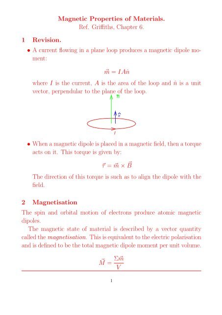
1 Revision.Magnetic Properties of Materials.Ref. Griffiths, Chapter 6.• A current flowing in a plane loop produces a magnetic dipole moment:⃗m = IAˆnwhere I is the current, A is the area of the loop and ˆn is a unitvector, perpendular to the plane of the loop.mnI• When a magnetic dipole is placed in a magnetic field, then a torqueacts on it. This torque is given by:⃗τ = ⃗m × ⃗ BThe direction of this torque is such as to align the dipole with thefield.2 MagnetisationThe spin and orbital motion of electrons produce atomic magneticdipoles.The magnetic state of material is described by a vector quantitycalled the magnetisation. This is equivalent to the electric polarisationand is defined to be the total magnetic dipole moment per unit volume.⃗M = Σ⃗mV1

3 Paramagnetic, Diamagnetic and Ferromagnetic materials.When materials are placed in a magnetic field, they become magnetised.Materials can be classified into three groups, on the basis of the sizeand the direction of the induced magnetisation.1. ParamagnetismPermanent dipoles which align with the field. Thermal disorderingplaces a limit on the degree of alignment, hence the effect is temperaturedependent. In a spatially varying field, such materials arepulled into the stronger part of the field.2. DiamagnetismDue to induced dipoles. The direction of the induced dipoles isopposite that of the inducing field - a result of Lenz’s law. In aspatially varying field, such materials are pushed out of the strongerpart of the field.3. FerromagnetismPulled strongly into field. Display non-linearity and a memoryof magnetic history (hysteresis). Correlated dipoles and domainstructure. The ferromagnetic elements are Fe, Ni Co and Gd (below16C). These are the materials we would normally think of asbeing attracted by a magnet.2

4 Bound Currents.When a material becomes magnetised, it generates a magnetic field.We can calculate these fields by replacing the magnetised material byequivalent bound currents.The bound currents are of two types; surface currents, given by:⃗K b = ⃗ M × ˆnand volume bound currents in the bulk material, given by:⃗J b = ∇ × ⃗ Mwhere ˆn is a unit vector normal to the surface at the point whereK b is to be calculated.See the simple derivation (Griffiths 6.2.2), ignore the full derivation(6.2.1).When using these expressions, keep in mind that the surface currentat some point on the surface, is given by the magnetisation atthat point. Likewise, the volume bound current at some point in thematerial is given by the curl of ⃗ M at that point.3

Example 1 (Griffiths pr. 6.12(a), p272)A long solid cylinder, radius R has a magnetisation ksẑ. Calculatethe bound currents.RK bMzSolutionFor the surface bound current:n = s⃗K b = ⃗ M × ˆnwhere ⃗ M = the magnetisation at the surface = kRẑ.and in this case ˆn = ŝ.For the volume bound current:Thus ⃗ K b = kRẑ × ŝ = kR ˆφ⃗J b = ∇ × ⃗ MNow ⃗ M has only a z component and this depends only on s. Hencethe only term we need to worry about in the curl is where the z componentis differentiated w.r.t. s.Thus J ⃗ b = − ∂M z∂s ˆφ = − ∂(ks)∂sˆφ = −k ˆφ4

Example 2.Calculate the magnetic field in the bar of the previous exampleB=0RLszBThe method is the same as that used to calculate the field in asolenoid. Use Ampere’s law and the bound currents. From symmetrywe guess the magnetic field lies along the z direction inside the bar andis zero outside. The dotted rectangle represents the Amperian loop.∮⃗B · ⃗dl = µ 0 I enchence: B L = µ 0 (kRL − k [R − s] L)⃗B = µ 0 ksẑ5

The H vectorThe total current flowing can be thought of as two parts, the freecurrent (from batteries etc.) and the bound currents. We can thenwrite Ampere’s law as:Thus ∇ ×( ⃗Bµ 0− ⃗ M∇ × ⃗ B = µ 0⃗ Jf + µ 0⃗ Jb)= µ 0⃗ Jf + µ 0 ∇ × ⃗ M= ⃗ J fThis leads to the definition of a new quantity which we will call theH vector; defined as:⃗H = ⃗ Bµ 0− ⃗ MUsing H, ⃗ Ampere’s is: ∇ × H ⃗ = J ⃗ f∫ ( ∮ ∫and since ∇ × H)⃗ · ⃗da = ⃗H · ⃗dl =⃗J f · ⃗dathe integral form is:∮⃗H · ⃗dl = I fencwhere I fenc is the free current enclosed by the path of the line integral.The units of H and M are amperes metres −1 .Note: It is tempting to think that we can calculate H ⃗ in just thesame way as we calculate B, ⃗ but just using the free currents. This isnot quite true. In order to calculate a vector we need to know bothits curl and its divergence. When calculating H ⃗ we usually use theintegral form of Ampere’s law and make assumptions about symmetry.The symmetry assumptions effectively replace the requirement of theknowledge of the divergence. Griffiths discusses this point in moredetail on page 273, section 6.3.2.6

Magnetic CoefficientsThe magnetic susceptibility relates ⃗ M to ⃗ H:⃗M = χ M⃗ HThe permeability relates ⃗ B and ⃗ H.⃗B = µ ⃗ HCombining these gives:µ = µ 0 (1 + χ M )The relative permeability is: µ r = µ µ 0The susceptibility tends to be used more when describing para- anddia- magnetic materials, while the permeabilbity is used for ferromagnetics.Typical values can be found in the text.Simple ExampleA long solenoid, with its axis parallel to z, has 1000 turns per metreand carries a current of 5 A. Calculate ⃗ B, ⃗ M and ⃗ H inside this solenoidif it is filled with:• Copper, with χ M = −0.96 × 10 −5• Aluminium, with χ M = 2.1 × 10 −5• Iron, with µ = 4.0 × 10 −5 NA −27

AnswerFirst calculate H ⃗ from ∮the free current.⃗H · ⃗dl = I f encHl = nIl⃗H = nIẑ (1)Then ⃗ M = χ M⃗ H (2)and ⃗ B = µ ⃗ H (3)We can now calculate the required values for each material fromequations (1), (2) and (3).This gives:Copper Aluminium Iron⃗H 5,000ẑ Am −1 5,000ẑ Am −1 5,000ẑ Am −1⃗M -0.048ẑ Am −1 0.105ẑ Am −1 1.59 × 10 6 ẑ Am −1⃗B 6.28 × 10 −3 ẑ T 6.28 × 10 −3 ẑ T 2ẑ TNotice that:1. ⃗ H is the same regardless of material. It depends only on the freecurrent.2. ⃗ B is not exactly the same in copper and aluminium. For copper,it is actually 0.9999904 times the value shown; and it is 1.000021times the value shown in aluminium.8

5 Boundary Conditions.(A simplified treatment of Griffiths page 273)It is useful to know the way in which B ⃗ and H ⃗ change as we crossthe interface between one material and another.Imagine what happens with the pillbox in the figure shown below,as its height shrinks to zero.BB n2n1Material 1Material 2We know that there can never be any net magnetic flux out of aclosed surface. The flux out of the top is the normal component of thefield multiplied by the area of the top. The flux in at the bottom isequal to the normal component of the field multiplied by the area ofthe bottom. Both areas are equal, so both normal components mustalso be equal.i.e. B n1 = B n2 (4)The normal component is unchanged as we move across an interface.9

For the tangential component look at the loop in the diagram below.Ht1Ht2Material 1Material 2lWe apply Ampere’s law, in the form involving ⃗ H, around this loopand imagine the loop to shrink to zero thickness.H t1 .l − H t2 .l = K f .l (5)For most materials there will be no free surface current at the interface(the exceptions are superconductors), thus in almost all cases:H t1 = H t2 or µ 1 B t1 = µ 2 B t2 (6)In summary, as we cross an interface between two materials, thenormal component of ⃗ B and the tangential component of ⃗ H do notchange.10

6 Ferromagnetism(Griffiths gives more detailed notes on this topic - pp 278-281.In the preceding sections we have assumed that the quantities ⃗ B, ⃗ Mand ⃗ H are linearly related to each other. In ferromagnetic materialsthis is not the case. The permeability of a ferromagnetic varies with thefield. In addition the magnetisation depends on the magnetic historyof the material, a phenomenon called hysteresis.The relation between B and H for typical ferromagnetic materialsis shown in the plot below. These plots are from hte laboratoryexperiment on magnetic fields.0.8HYSTERISIS LOOPS0.60.40.2B (arb. units)0−0.2−0.4−0.6−0.8−0.3 −0.2 −0.1 0 0.1 0.2 0.3 0.4H (arb. units)When M is plotted against H similar plots are obtained.Such plots are called hysteresis plots, or B-H curves. The field remainingwhen H is reduced to zero is called the remanent field. Thevalue of H required to reduce B to zero after full megnetisation iscalled the coercive field.11

The basis of the behaviour of ferromagnetism is a domain structureand dipole interactions.In ferromagnetic materials, neighbouring dipoles align with eachother in small regions called domains. When an external field is applied,the domain boundaries move. Domains aligned with the fieldgrow, while others shrink. When the external field is removed, thedomain boundaries do not move fully back to their original positions -this is hysteresis. The magnetic proeprties of a ferromagnetic materialdepend on its history.12