special issue for the 18 nordic seminar on computational mechanics ...

VOL. 38, 2005, Nro 3SPECIAL ISSUE FOR THE <strong>18</strong> TH NORDIC SEMINAR ONCOMPUTATIONAL MECHANICSOCTOBER, 27 TH – 30 TH 2005RAKENTEIDEN MEKANIIKAN SEURA RYFINNISH ASSOCITATION FOR STRUCTURAL MECHANICS1

R A K E N T E I D E N M E K A N I I K A N S E U R A R.Y.FINNISH ASSOCIATION FOR STRUCTURAL MECHANICSJOHTOKUNTAADMINISTRATIVE BOARDJUHA PAAVOLA, prof. (puheenjohtaja), TKK/Rakenteiden mekaniikkaTAPIO AHO, dipl. ins., Ins.tsto Magnus Malmberg OyJOUNI FREUND, tekn.tri, TKK/LujuusoppiJUHANI KOSKI, prof., TTY/Tekn. mek. ja optimointiKARI KOLARI, dipl. ins., TKK/LujuusoppiREIJO LINDGREN, dipl. ins., CSC-Tieteellinen laskentaSEPPO ORIVUORI, tekn.lis, Enprima OyILMO SIPILÄ, dipl. ins., Ins.tsto Ilmo SipiläJUKKA TUHKURI, prof., TKK/LujuusoppiMATTI RANTA, prof., kunniapuheenjohtajaTOIMISTOOFFICESAMI PAJUNEN, asiamies, puh. 040 900 4501ELSA NISSINEN-NARBRO, kanslisti/jäsenasiat, puh. (09) 451 3701JÄSENETMEMBERSHENKILÖJÄSENET 176OPISKELIJAJÄSENET 3YHTEISÖJÄSENET:Aaro Kohonen OyFinnmap Consulting OyIns.tsto JP-Kakko OyIns.tsto Magnus Malmberg OyIns. tsto Pontek OyIns.tsto Pöysälä & Sandberg OyTKK/LaivalaboratorioKCI Konecranes International PlcKonecranes VLC OyKPM-Engineering OyNokian Renkaat OyjOptiplan OySuomalainen Insinööritoimisto SITO OyPohjois-Karjalan AMKOSOITE:3826Teknillinen korkeakoulu, Rakennus- ja ympäristötekniikan osasto,Rakentajanaukio 4 A, PL 2100, 02015 TKK, puh. (09) 451 3701, telefax (09) 451ADDRESS: Helsinki University of Technology, Department of Civil and EnvironmentalEngineering, Rakentajanaukio 4 A, P.O.Box 2100, FIN-02015 HUT, Finland.tel. (358-9) 451 3701, telefax (358-9) 451 3826http://rmseura.tkk.fi/

www.ruukki.comIf you see <strong>the</strong> nameRuukki instead ofRautaruukki, Rannila,Fundia Rein<strong>for</strong>cing,Gasell or Asva, you areactually seeing more.

Call <strong>for</strong> papersAccidents and safety in construction sectorConstructionSAFETYMay10-12, 2006Helsinki, Finland2006Finnish Association of Civil EngineersThe construction industry is one of <strong>the</strong>most hazardous workplaces in <strong>the</strong> world.Mistakes during construction often leadto very negative and unwanted resultslater - to loss of property or even humanlives. Such situations may be caused ei<strong>the</strong>rby natural disasters and environmentalchanges or human errors, whe<strong>the</strong>rdeliberate or involuntary.The Finnish construction industry, <strong>special</strong>istorganizations and authorities havediscussed ways to improve <strong>the</strong> situationand found exchange of in<strong>for</strong>mation, circulationof best practices, learning fromcases and brainstorming with colleaguesand stakeholders to be one good way toproceed. The Finnish Association of CivilEngineers RIL, as an impartial networkof experts, has decided to open a timewindow and plat<strong>for</strong>m <strong>for</strong> an open discussionand exchange of views betweenEuropean, Finnish and global industrymembers by organizing a conferencewhere <strong>the</strong>se <strong>issue</strong>s can be presented anddiscussed .This is an open call <strong>for</strong> experts,practioners, researchers and o<strong>the</strong>r professionalsdealing with structural andoccupational safety to step ahead, exchange<strong>the</strong>ir knowledge and in<strong>for</strong>mationabout <strong>the</strong>se important <strong>issue</strong>s and tolearn, how to make construction industrya safe industry and built environmenta safe place to live!More in<strong>for</strong>mation:www.ril.fi/safety2006or kaisa.venalainen@ril.fi

PrefaceThese proceedings contain <strong>the</strong> papers presented at <strong>the</strong> <strong>18</strong> th Nordic Seminar onComputational Mechanics, held at Silja Serenade ferry travelling between Helsinki andStockholm, <strong>the</strong> Capitals of Finland and Sweden, and hosted by Helsinki University ofTechnology, Espoo, Finland, on 27-30 October 2005.The <strong>seminar</strong>s are organized annually by <strong>the</strong> Nordic Association of ComputationalMechanics (NoACM). The NoACM was founded in 1988 with <strong>the</strong> objective tostimulate and promote research and practice in computational mechanics, to foster <strong>the</strong>interchange of ideas among <strong>the</strong> various fields contributing to computational mechanics,and provide <strong>for</strong>ums and meetings <strong>for</strong> dissemination of knowledge in computationalmechanics. Younger researchers, including doctorate students etc. are e<strong>special</strong>lyencouraged to participate at <strong>the</strong>se <strong>seminar</strong>s. The member countries of NoACM are <strong>the</strong>Nordic countries (Denmark, Finland, Iceland, Norway and Sweden) and <strong>the</strong> Balticcountries (Estonia, Latvia and Lithuania). NoACM is a subchapter of <strong>the</strong> InternationalOrganization <strong>for</strong> Computational Mechanics (IAC) and <strong>the</strong> European Community onComputational Methods in Applied Sciences (ECCOMAS).The responsibility <strong>for</strong> organizing this year’s <strong>seminar</strong> was assigned by NoACM toLaboratories of Structural Mechanics and Mechanics of Materials, Helsinki Universityof Technology. Traditionally, <strong>the</strong> <strong>seminar</strong>s have been organized in academic universitycircumstances. To reserve <strong>for</strong> participants more time to have with each o<strong>the</strong>r and toprovide <strong>the</strong> common time with more com<strong>for</strong>ts, this time <strong>the</strong> <strong>seminar</strong> will be arranged in<strong>the</strong> ferry. The <strong>seminar</strong> contains five invited lectures and 38 contributed presentationsdivided into 10 separate sessions of which some are parallel ones. In this volume, <strong>the</strong>invited keynote lectures are placed first and after that comes <strong>the</strong> contributed papers in<strong>the</strong> order of <strong>the</strong> <strong>seminar</strong> program.On behalf of <strong>the</strong> organizers, we’d like express our gratitude to all contributors of <strong>the</strong><strong>seminar</strong>, <strong>the</strong> invited and contributed speakers <strong>for</strong> <strong>the</strong>ir ef<strong>for</strong>t in preparing talks,presentations and papers, and to those all who have helped in practical arrangements.Finally, we thank all <strong>the</strong> sponsors, Ruukki, KCI Konecranes PLC, VTT-TechnicalResearch Centre of Finland, and Finnish Association of Civil Engineers, who havehelped us to make this <strong>seminar</strong> true. Particularly, <strong>the</strong> Finnish Association of StructuralMechanics, deserves to be mentioned <strong>for</strong> serving a great <strong>for</strong>um to publish <strong>the</strong> <strong>seminar</strong>abstracts in <strong>the</strong> <strong>special</strong> <strong>issue</strong> devoted <strong>for</strong> <strong>the</strong> <strong>seminar</strong>.Espoo, 21 October 2005The editors

Program CommitteeKjell Magne Mathisen, NorwayTrond Kvamsdal, NorwayAnders Eriksson, SwedenGöran Sandberg, SwedenRoland Rikards, Latvia ( Baltic countries )Juha Paavola, FinlandJouni Freund, FinlandNiels Olhoff, DenmarkJens Sørensen, DenmarkLocal Organizing CommitteeJuha PaavolaJouni FreundEnnio ZuccaroNSCM<strong>18</strong> secretariatEnnio ZuccaroLaboratory of Structural MechanicsHelsinki University of TechnologyPO Box 210002015 TKKFINLANDPhone: +358 9 451 3711Fax: +358 9 451 3826

Table of contentsKeynote lecturesJukka Tuhkuri Discrete element simulations in ice engineering 1Jens Wal<strong>the</strong>r Numerical Simulation of Nano-, Meso, Macro- and Multiscale Fluid 9DynamicKnut-Andreas Lie Multiscale methods <strong>for</strong> flow in porous media 19Ragnar Larsson Inverse Discontinuity Formulation of Fracture 27Tarmo Soomere Lessons in wave <strong>the</strong>ory from <strong>the</strong> Indian Ocean Tsunami of Millenniumand from <strong>the</strong> Baltic Sea Storm Surge of Century31Parallel session I : fractureJaan Lellep Inelastic conical shells with cracks 24Mikko Lyly Simulation of quasi-static crack growth by using <strong>the</strong> method 37Timo Saksala Explicit FE-procedure <strong>for</strong> Numerical Modeling of Rock Fracture underDynamic Indentation41Parallel session I : applicationsMats Larson Residual Based Approximations of Fine Scales in Variational Multiscale 45Approximations of Navier-Stokes EquationsMats Larson Adaptive Simulation of Multiphysics Problems 47Trond Kvamsdal Algorithms <strong>for</strong> fluid-structure interaction of flow around two or morecylinders with large relative motions.49Ordinary session IAnders Kristensen Finite element analysis of jar connections : Modeling considerations 51Kilwa Ärölä De<strong>for</strong>mation of a Paper Roll Loaded Against a Nip Roller 55Tellervo Brandt Comparison between Approaches to Explicit Filtering in Large EddySimulation 59FeliksasMa<strong>the</strong>matica Modelling of Biosensors with Per<strong>for</strong>ated and Selective 63Ivanauskas MembranesJohn Öström Modeling Aircraft Ground Behavior into a Flight Simulation 67Parallel session II : numericsAntti Niemi Benchmark study: MITC4-S and boundary layer-type de<strong>for</strong>mations 71Jarkko Niiranen Computational results <strong>for</strong> <strong>the</strong> superconvergence and postprocessing of 75MITC plate elementsJuhani Pitkäranta Locking-Free Plate Elements at Free Boundary 79Gunnar Tibert Finding <strong>the</strong> most efficient rotation-free triangular shell element 83Marcus Rüter A Posteriori Error Estimates in Linear Elastic Fracture Mechanics basedon Different FE-Solution Spaces <strong>for</strong> <strong>the</strong> Primal and <strong>the</strong> Dual Problem87Parallel session II : applicationsPentti Varpasuo FPK-equation solutions <strong>for</strong> stochastic structural response 91Helle Hein The Effect of Delamination on <strong>the</strong> Natural Frequencies of <strong>the</strong> Composite 97Beams on Two-Parameter FoundationReetta Karjalainen Fatigue life prediction of polymer covered roll 101Lena Strömberg Extension of ASME regulatory <strong>for</strong> validation of dynamical calculation 105when deviations in as-buildtJani Paavilainen Forces Between Joined Discrete Particles in Discrete Element Method 109

Parallel session III : numericsMika Juntunen A Finite Element Method <strong>for</strong> General Boundary Condition 113Sergey Korotov New Tecnologies <strong>for</strong> Control of Local Errors in Engineering 117Computations by FEMSanna Mönkölä Solution of <strong>the</strong> Helmholtz equation with controllability and spectralelement methods121Parallel session III : educationJouni Freund Vectors and tensors with matrix manipulations 125Juha Paavola Virtual Work, Lagranges Equations and Finite Elements 129Lena Strömberg Inertia and related topics of education in mechanics 133Parallel session IV : materialsAnders Lyckegaard Stress evaluation in sandwich structures near tri-material wedge 135Tuomas Peräkylä Identification of Material Parameters of a Polymer 139Lena Strömberg Non-local plasticity model <strong>for</strong> fibre rein<strong>for</strong>ced concrete 143Antti-Jussi Vuotikka Time-Temperature Superposition Method <strong>for</strong> Polyester Resin 149Johan Clausen Slope safety calculation with a non-linear Mohr criterion using finiteelement method153Parallel session IV : applicationsJohnny Jacobsen Shape Optimisation of Core Interfaces in Sandwich Structures 157Sergey Sorokin On wave attenuation in sandwich plates loaded by a layer of viscous fluid 161Gunnar Tibert Flexibility Evaluation of Prestressed Kinematically Indeterminate 165FrameworksJukka Toivanen On shape sensitivity analysis with unstructured grids 169Jussi Jalkanen Space Frame Optimization Using PSO 173Seminar closureBastian Ebbecke Simulation of Stress Adaptive Bone Remodelling 177Index of authorsList of participantsSeminar programme

Discrete Element Simulations in Ice EngineeringJukka TuhkuriLaboratory <strong>for</strong> Mechanics of MaterialsHelsinki University of Technology, Espoo, Finlande–mail: jukka.tuhkuri@tkk.fiSummary The ice load on an engineering structure depends on <strong>the</strong> de<strong>for</strong>mation and failure process ofsea ice. As several ice features and ice failure processes are discontinuous in nature, it is tempting to study<strong>the</strong> ice load problem by using a discontinuous approach. Discrete element method (DEM) is one of <strong>the</strong>techniques that model <strong>the</strong> dynamics of a system of discrete particles. This paper gives a review of a groupof ice problems and <strong>the</strong>ir analysis with DEM.IntroductionDetermination of ice loads on ships and offshore structures is an important technical challenge.Ice <strong>for</strong>ces acting on a structure are due to relative movement between <strong>the</strong> structure and ice and <strong>the</strong>sequential failure process of <strong>the</strong> ice feature. Typical sea ice features are sheets of level ice, ridgesand rubble fields. Both ridges and rubble fields are piles of ice blocks, but ridges have an elongated<strong>for</strong>m. Ridges and rubble fields <strong>for</strong>m when two ice sheets, driven by winds and currents, collide. In<strong>the</strong> Baltic, ridges more than 10 meters deep are common.A central hypo<strong>the</strong>sis in traditional solid mechanics states that a body under consideration is continuousand remains continuous under <strong>the</strong> action of external <strong>for</strong>ces. However, ice mechanics is oneof <strong>the</strong> engineering fields where this continuum description may not be <strong>the</strong> most appropriate, anda discontinuum approach should be used instead. Figure 1 shows two important ice engineeringproblems. The key features of <strong>the</strong> ice load cases shown are <strong>the</strong> discontinuous nature of both <strong>the</strong>pile of ice blocks and <strong>the</strong> failure process of ice. When an ice sheet loads a structure as in Figure1(a), <strong>the</strong> originally intact ice sheet breaks into discrete ice blocks which accumulate in <strong>the</strong> icestructureinterface and thus affect <strong>the</strong> failure process. On <strong>the</strong> o<strong>the</strong>r hand, when a structure indentsa ridge or an ice rubble pile as in Figure 1(b), <strong>the</strong> load on <strong>the</strong> structure is due to rearrangement of<strong>the</strong> discrete ice blocks, in addition to possible failure of <strong>the</strong> ice blocks.(a)Figure 1: (a) Sketch of en ice sheet failure against an inclined marine structure. (b) Snapshot of a DEMsimulation of an indentor moving down into a floating layer of ice blocks [1].The discrete element method (DEM) is a numerical tool used to simulate a system of particles.DEM is based on <strong>the</strong> concept that individual material elements are considered to be separate and,(b)1

if connected, are connected along <strong>the</strong>ir boundaries by appropriate interaction laws. An importantaspect of <strong>the</strong> discrete element method is that <strong>the</strong> particles may fracture and fragment, thusincreasing <strong>the</strong> total number of bodies during a simulation. In a discrete element simulation, <strong>the</strong>interaction and behavior of individual particles will result into emergent physical properties of <strong>the</strong>particle assembly. A DE approach can be useful in cases where <strong>the</strong> constitutive behavior of a particleassembly is not known. In addition to ice mechanics, DEM has been applied to de<strong>for</strong>mationof granular materials, rock mechanics, fragmentation of solids, as well as structural failure andcollapse [2][3][4]. This paper first will introduce <strong>the</strong> discrete element method and <strong>the</strong>n describesome engineering problems analysed with DEM. The goal is not to give an extensive literaturereview, but to highlight a few important applications.The discrete element methodIn essence, a discrete element simulation is a computer program that models <strong>the</strong> nonlinear dynamicsof a system of particles. The <strong>for</strong>ces on each particle are calculated at each time step and <strong>the</strong>particles are moved to new locations with new velocities that depend on <strong>the</strong> <strong>for</strong>ces. Newtonianmechanics is assumed to describe <strong>the</strong> particle motions. A DEM program has <strong>the</strong> following tasks:1. Store <strong>the</strong> position, orientation, velocity, and shape of each particle.2. Find <strong>the</strong> neighboring particles.3. Find <strong>the</strong> contact geometry (overlapping areas) between <strong>the</strong> neighboring particles.4. Determine <strong>the</strong> contact <strong>for</strong>ces between particles, i.e. add <strong>the</strong> physical properties of <strong>the</strong> particlesinto <strong>the</strong> simulation.5. Determine whe<strong>the</strong>r any particle will fracture into new particles.6. Solve <strong>the</strong> equations of motion of <strong>the</strong> particles and move each to a new position with a newvelocity and orientation.7. Analyse <strong>the</strong> variables of interest and construct a visual record of <strong>the</strong> systems motion.The second and third tasks, dealing both with contact detection, are time consuming. For radiallysymmetric particles (disks and spheres) it is a trivial task, but <strong>for</strong> polygonal or polyhedral particles<strong>the</strong> task is a complex exercise in computational geometry. Presumably <strong>for</strong> this reason, <strong>the</strong> majorityof DE simulations have been per<strong>for</strong>med by using disks or spheres. However, in many physicalproblems <strong>the</strong> particles are not symmetric and <strong>the</strong> particle shape is an important feature of a granularassembly [5][6][1].The fourth task is to determine <strong>the</strong> contact <strong>for</strong>ces between particles. The traditional method inDEM has been to treat each particle as a rigid body, calculate <strong>the</strong> overlap of <strong>the</strong> bodies and torelate <strong>the</strong> overlap depth δ with contact <strong>for</strong>ce by using simple spring and dashpot models. Forexample, <strong>the</strong> normal contact <strong>for</strong>ce F n in compression is <strong>the</strong>nF n = k n δ + c n ˙δ (1)where k n is <strong>the</strong> contact stiffness and c n is <strong>the</strong> contact damping. This widely used model is somewhatcontroversial, because it is not clear what k n and c n are. For elastic spheres, k n can be2

defined by using <strong>the</strong> Hertz contact model, but <strong>for</strong> o<strong>the</strong>r particle shapes, no general k n exist. Thus,a more recent approach is to use a combined finite-discrete element method where each particle ismodelled by using FEM [4][7].The contact <strong>for</strong>ce in Equation 1 is <strong>for</strong> compression only. In problems dealing with an assembly ofdiscrete particles, <strong>the</strong> normal <strong>for</strong>ce in tension vanishes. However, also tensile contact <strong>for</strong>ces canbe easily taken into account in DEM.Research of ice engineering problems with DEMProblems dealing with ice fields comprising of discrete ice floesThe early applications of DEM in ice problems concentrated in modelling <strong>the</strong> convergent behaviorof systems of circular ice floes in two dimensions (2D) [6] [8]. In <strong>the</strong>se studies, <strong>the</strong> goal was toexamine <strong>the</strong> constitutive equations of ice cover in large scale. Engineering applications of thisproblem include simulations of river ice transport phenomena [9], <strong>for</strong>ces exerted on a boom whenit is pulled through a broken ice sheet [10] and <strong>the</strong> behavior of a ship moored in broken ice (Figure2) [11]. Later, three dimensional (3D) simulations have shown that <strong>the</strong> floes start to overlap eacho<strong>the</strong>r when <strong>the</strong> floes are packed on <strong>the</strong> water surface at an average concentration of about 80 %by area [12]. In o<strong>the</strong>r words, when <strong>the</strong> concentration reaches 80 %, <strong>the</strong> problem becomes 3D andcannot be modelled with 2D models.Figure 2: Snapshot of a 2D DEM simulation of a ship (left) moored in broken ice moved by a current [11].Figure 3 shows a snapshot from 3D ice floe field simulations in which a floating layer of circularfloes, confined in a rectangular channel, was compressed by a pusher moving at a constant speed[12]. The accuracy of <strong>the</strong> simulations was assessed by comparison with a series of similar physicalexperiments per<strong>for</strong>med in a refrigerated basin. Figure 4(a) shows <strong>the</strong> <strong>for</strong>ces on <strong>the</strong> pusher obtainedin <strong>the</strong> experiments and simulations with two ice thicknesses. Three distinct regions are evident in<strong>the</strong> <strong>for</strong>ce-displacement, F ∗ (X ∗ ), graphs. During <strong>the</strong> first period (X ∗ < 6), <strong>the</strong> <strong>for</strong>ces increase as<strong>the</strong> floes are herded toward <strong>the</strong> far end of <strong>the</strong> channel. The pusher <strong>for</strong>ce at X ∗ = 6 represents<strong>the</strong> strength of <strong>the</strong> 2D consolidated surface layer of horizontal floes. During <strong>the</strong> second period6 < X ∗ < 35, <strong>the</strong> F ∗ (X ∗ )-record is characterised by <strong>the</strong> resistance of <strong>the</strong> floes to rotation andrafting, but also to frictional contact with <strong>the</strong> channel sides. The third period, X ∗ > 35 beginswhen <strong>the</strong> entire initial surface layer of floes has failed. Following this comparison, <strong>the</strong> computermodel was used to explore <strong>the</strong> effect of variations in channel length and width, <strong>the</strong> ratio of floediameter to thickness, floe on floe friction coefficients, and <strong>the</strong> distribution of floe diameters on<strong>the</strong> <strong>for</strong>ce required to compress <strong>the</strong> floes. As an example, <strong>the</strong> frictional <strong>for</strong>ce at <strong>the</strong> channel sides,3

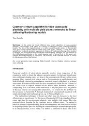
Figure 3: Snapshot of a 3D DEM simulation of a pusher (right) compressing a floating layer of ice floes[12].which is an artifact of <strong>the</strong> experimental setup and does not appear in nature, can be removed in <strong>the</strong>DE simulations by using periodic boundary conditions. Figure 4(b) shows <strong>the</strong> simulated F ∗ (X ∗ )-record <strong>for</strong> two channel lengths L ∗ with periodic boundary conditions. Comparison between <strong>the</strong>results shown in Figures 4(a) and 4(b) suggest that <strong>the</strong> positive slope in <strong>the</strong> F ∗ (X ∗ )-record at5 < X ∗ < 35 in Figure 4(a) is caused by <strong>the</strong> channel edge friction.A 3D DEM simulation of an ice floe field has also been used to model ship channel ice resistance[13]. That was done by replacing <strong>the</strong> pusher shown in Figure 3 by a ship shaped object.The mechanical properties of ice ridge keels are important in<strong>for</strong>mation <strong>for</strong> ridge load calculations.For over a decade, ice rubble problems have been studied with DEM in 2D [6] [14][1]. Snapshotof a simulation of ridge keel punch test was shown in Figure 1(b) and Figure 5 shows <strong>the</strong><strong>for</strong>ce-displacement graph of this simulation, toge<strong>the</strong>r with results obtained by using o<strong>the</strong>r particleshapes. These simulations suggest that <strong>the</strong> ridge keel indentation load is highest <strong>for</strong> <strong>the</strong> rubble pile<strong>for</strong>med from rectangular particles and lowest <strong>for</strong> a pile <strong>for</strong>med from circular particles. However,<strong>the</strong> shape of <strong>the</strong> <strong>for</strong>ce-displacement graph appears not to be strongly affected by <strong>the</strong> particle shape.The differences in ice ridge analyses, per<strong>for</strong>med by using a discontinuum approach (DEM) or amore traditional continuum approach, can now be highlighted. In a DE model, <strong>the</strong> ridge behavioris defined by local scale parameters through de<strong>for</strong>mation, failure and interaction of individual iceblocks. These local scale parameters are, <strong>for</strong> example, <strong>the</strong> elastic modulus E of ice and <strong>the</strong> ice-icefriction coefficient µ. The traditional way to study ice ridge loads is to model <strong>the</strong> ice mass withmodels based on soil mechanics. For example, in <strong>the</strong> Mohr-Coulomb model <strong>the</strong> ridge strength isdefined with friction angle φ and cohesion c. These parameters describe behavior of <strong>the</strong> ridge asa whole. It is reasonable to assume that if <strong>the</strong> number of ice floes in a ridge is high enough, <strong>the</strong>continuum approach should give acceptable results. However, <strong>the</strong> minimum number of ice blocksrequired to fulfill <strong>the</strong> continuum approach is not known. Ano<strong>the</strong>r point of interest is to consider<strong>the</strong> parameters describing ridge behavior in <strong>the</strong> two approaches. Currently, it is not totally clearwhat are <strong>the</strong> most important local scale parameters (µ, E, block shape, etc.), nor it is known whatare <strong>the</strong> relationships between <strong>the</strong> local scale parameters and <strong>the</strong> Mohr-Coulomb model.4

(a)Figure 4: (a) Nondimensional pusher <strong>for</strong>ce versus displacement as measured in experiments (model) andsimulations (simul) shown in Figure 2. h is ice thickness. (b) Nondimensional pusher <strong>for</strong>ce versus nondimensionalpusher displacement <strong>for</strong> two channel lengths L ∗ with periodic boundary conditions [12].(b)Problems dealing with ice sheetsThe failure of ice cover against a marine structure is a fragmentation process where a solid disintegratesinto discrete particles which <strong>the</strong>n interact with each o<strong>the</strong>r and pile-up against <strong>the</strong> structure(Figure 1(a)). DEM appears to be well suited to this kind of problems, but only a few studies havebeen per<strong>for</strong>med, e.g. [15][16]. Ano<strong>the</strong>r ice pile-up process is ridging. Ice ridges <strong>for</strong>m when twoice sheets are driven toge<strong>the</strong>r, ice blocks break off <strong>the</strong> sheets and pile-up to <strong>for</strong>m a ridge. Ridge<strong>for</strong>mation from two thin sheets [17] as well as from a thin sheet breaking against a thick sheet [<strong>18</strong>]have been studied with DEM. Rafting is a process closely related to ridging. Rafting is <strong>the</strong> simpleoverriding of one ice sheet by ano<strong>the</strong>r ice sheet.From an engineering point of view, ridging and rafting are important processes, as <strong>the</strong>y define <strong>the</strong>horizontal <strong>for</strong>ce an ice sheet can transmit. In o<strong>the</strong>r words, ridging and rafting define <strong>the</strong> horizontalstrength of an ice sheet and thus give an upper limit <strong>for</strong> <strong>the</strong> ice load on a marine structure.Figure 6 shows snapshots from DEM simulation showing rafted and ridged ice. In that two dimensionalsimulation [17], two identical ice sheets were pushed toge<strong>the</strong>r. Each ice sheet was composedof two thicknesses of ice and <strong>the</strong> ratio of thicknesses was varied to obtain degrees of inhomogeneity.Again, <strong>the</strong> accuracy of <strong>the</strong> simulations was assessed by comparison with a series of similarphysical model scale experiments. Both <strong>the</strong> experiments and <strong>the</strong> simulations showed that homogeneousice sheets tend to raft and inhomogeneous ice sheets tend to <strong>for</strong>m ridges. Following <strong>the</strong>comparison, <strong>the</strong> computer model was used to per<strong>for</strong>m simulations to study <strong>the</strong> ridging and rafting<strong>for</strong>ces and to systematically explore <strong>the</strong> effect of <strong>the</strong> thickness and thickness inhomogeneity on<strong>the</strong> likelihood of occurrence of ridging and rafting. Compared to <strong>the</strong> physical experiments, <strong>the</strong>DE simulations provided a low cost alternative to systematic parametric studies. In addition, withsimulations it is easier to isolate <strong>the</strong> effect of a single variable in a physical process. Comparisonof <strong>the</strong> measured and calculated <strong>for</strong>ces (Figure 7) showed that <strong>the</strong> average simulation <strong>for</strong>ces underestimated<strong>the</strong> average experimental <strong>for</strong>ces by about 50 %. This difference is most likely due to <strong>the</strong>two dimensionality of <strong>the</strong> computer model, and highlights <strong>the</strong> need <strong>for</strong> 3D simulation tools.5

F [kN/m]15105Rect. 1:6Rect. 1:3SquaresDisks00 0.5 1 1.5 2 2.5 3δ [m]Figure 5: Force-displacement records from punch test simulations, shown in Figure 1(b), with differentparticle shapes [1].(a)Figure 6: Scenes from a DEM simulation showing (a) rafted and (b) ridged ice [17].(b)Summary and discussionIn this paper <strong>the</strong> discrete element method and some typical problems in ice engineering have beenshortly reviewed. It was argued that <strong>the</strong>re are ice engineering problems which should be analysedby using a discontinuous approach, ra<strong>the</strong>r than <strong>the</strong> more traditional continuum approach. First,several ice features comprise of discrete ice floes and, in addition, often <strong>the</strong> individual ice floesare large compared to <strong>the</strong> size of <strong>the</strong> ice feature. As an example, an ice ridge may be <strong>for</strong>medthrough stacking of less that ten layers of ice. Second, <strong>the</strong> ice failure process is a discontinuousfragmentation process. An example of this kind of problem is failure of an ice cover against astructure.The studies reviewed have demonstrated <strong>the</strong> usefulness of DEM in ice engineering. DEM can beused in similar tasks than model scale experiments but, more importantly, DEM can be effectivelyused to study <strong>the</strong> effects of changing a single parameter.While DEM is well established and has been applied to different kinds of problems, <strong>the</strong> applicationof DEM is still expanding, probably because of <strong>the</strong> increase in available computing power. One of<strong>the</strong> interesting new trends in DEM is <strong>the</strong> development of combined finite-discrete element method[4], where each discrete element is modelled with FEM. While this is computationally demanding,it offers possibilities to model <strong>the</strong> particle-particle contacts in a more rigorous way than can bedone with a spring and dashpot model, see Equation 1.6

Figure 7: Force-displacement records from 3D physical experiments (model tests) and similar 2D ridgesimulations shown in Figure 5(b) [17].References[1] J. Tuhkuri and A. Polojärvi. Effect of particle shape in 2D ridge keel de<strong>for</strong>mation simulations. In Proc.<strong>18</strong>th Int. Conf. on Port and Ocean Engineering Under Arctic Conditions (POAC’05), Potsdam, NewYork, USA, Vol. 2, pp. 939-948, (2005).[2] P.A. Cundall and O.D.L. Strack. A discrete numerical model <strong>for</strong> granular assemblies. Geotechnique,bf 29, 47–65, (1979).[3] O.R. Walton. Explicit particle dynamics model <strong>for</strong> granular materials. In Proc. of 4th Int. Conf. onNumerical Methods in Geomechanics, Edmonton, Canada, 8 p. (1982).[4] A. Munjiza. The Combined Finite-Discrete Element Method. Wiley, (2004).[5] P.W. Cleary and M.L. Sawley. DEM modelling of industrial granular flows: 3D case studies and <strong>the</strong>effect of particle shape on hopper discharge. Applied Ma<strong>the</strong>matical Modelling, 26, 89–111, (2002).[6] M.A. Hopkins and W.D. Hibler. On <strong>the</strong> strength of geophysical scale ice rubble. Cold Regions Scienceand Technology, 19, 201–212, (1991).[7] A. Polojärvi. Combined Finite-Discrete Element Method in 3D Ridge Keel De<strong>for</strong>mation Simulations.Thesis <strong>for</strong> <strong>the</strong> degree of M.Sc. (Eng.). Helsinki Univ. of Technology, Faculty of Mechanical Engineering,86 p. (2005).[8] M. Sayed, V.R. Neralla and S.B Savage. Yield conditions of an assembly of discrete ice floes. In. Proc.of <strong>the</strong> 5th Int. Offshore and Polar Engineering Conference, The Hague, The Ne<strong>the</strong>rlands, Vol. II, pp.330-335, (1995).[9] M. Babic, H.T. Shen and G. Bjedov. Discrete element simulations of river ice transport. In. Proc. ofIAHR Symposium on Ice, Espoo, Finland, Vol. 1, pp. 564–574, (1990).[10] S. Løset. Discrete element modelling of a broken ice field, Parts I & II. Cold Regions Science andTechnology, 22, 339–360, (1994).[11] E. Hansen. A discrete element model to study marginal ice zone dynamics and <strong>the</strong> behaviour of vesselsmoored in broken ice. Dept. of Marine Hydrodynamics, Norvegian Univ. of Science and Technology,MTA-report 1998:124, 159 p. (1998).7

[12] M.A. Hopkins and J. Tuhkuri. Compression of floating ice fields. Journal of Geophysical Research,104, 15,815–15,825, (1999).[13] R. Haukioja. Simulation of ships channel ice resistance. Thesis <strong>for</strong> <strong>the</strong> degree of M.Sc. (Eng.).Helsinki Univ. of Technology, Faculty of Mechanical Engineering, 74 p. (2000).[14] E. Evgin, R.M.W. Frederking and C. Zhan. Distinct element modelling of ice ridge <strong>for</strong>mation. InProc. 11th OMAE Symp., Calgary, Canada, Vol. IV, pp. 255-260, (1992).[15] E. Evgin and C. Zhan. Distinct element modelling in ice mechanics. Dept. of Civil Engineering,University of Ottawa, Report from Finnish/Canadian Joint Research Project No. 5., 80 p. (1991).[16] M.A. Hopkins and W.D. Hibler. Onshore ice pile-up: a comparison between experiments and simulations.Cold Regions Science and Technology, 26, 205–214, (1997).[17] M.A. Hopkins, J. Tuhkuri and M. Lensu. Rafting and ridging of thin ice sheets. Journal of GeophysicalResearch, 104, 13,605–13,613, (1999).[<strong>18</strong>] M.A. Hopkins. On <strong>the</strong> ridging of intact lead ice. Journal of Geophysical Research, 99, 16,351–16,360,(1994).8

Numerical Simulation of Nano-, Meso-, MacroandMultiscale Fluid DynamicsJ. H. Wal<strong>the</strong>rDepartment of Mechanical Engineering, Fluid Mechanics SectionDanish Technical University, Kgs. Lyngby, Denmarke–mail: jhw@mek.dtu.dkalso at: Institute of Computational ScienceETH Zürich, CH-8092, Switzerlande–mail: wal<strong>the</strong>r@inf.ethz.chP. KoumoutsakosInstitute of Computational ScienceETH Zürich, CH-8092, Switzerlande–mail: petros@inf.ethz.chSummary We present algorithms and numerical simulations of fluid flow at <strong>the</strong> nano-, meso- and macroscale.The techniques involve nonequilibrium molecular dynamics simulations of fluids in nanoscale confinement,dissipative particle dynamics <strong>for</strong> fluids at <strong>the</strong> mesoscale, and smooth particle hydrodynamics and particlevortex methods <strong>for</strong> compressible and incompressible macroscale fluid dynamics. We couple <strong>the</strong> nano- andmacroscale descriptions using a Schwarz alternating procedure and effective boundary wall <strong>for</strong>ces to minimize<strong>the</strong> artifacts introduced by <strong>the</strong> interface between <strong>the</strong> two regions. This procedure is extended to <strong>the</strong>mesoscale model and includes <strong>the</strong> inherent fluctuations at this length scale. A unifying particle descriptionis used thoughout in <strong>the</strong> framework of massively parallel hybrid particle-mesh library.IntroductionParticle methods provide a powerful, unifying description of discrete and continuum mechanics[17] with applications that that range from atomistic systems using molecular dynamics (MD)simulations, through agglomerations of atoms and molecules at meso-scopic time and lengthscales using dissipatitive particle dynamics (DPD), and continuum description of fluid and solidmechanics using vortex particle method (VM) and smooth particle hydrodynamics (SPH), to planetarysystems invoking Barnes-Hut [1] and hybrid particle-mesh methods [13].The kinematic relations governing <strong>the</strong>se different systems share many common features and mayoften be described in terms of short- and long-range interaction potentials. The latter includes <strong>the</strong>omnipresent potential governing electrostatics, gravitation, and “induced fluid motion” in vortexparticle methods. The computational cost associated with <strong>the</strong> evaluation of <strong>the</strong> -potential<strong>for</strong>mally scales as ¡£¢¥¤ , where ¡£¢¥¤ denotes <strong>the</strong> number of computational elements/particles, and¦¨§©£ ©severely limits <strong>the</strong> computational efficiency of <strong>the</strong>se methods. Fast Multipole Methods (FMM)[12] have been developed to reduce <strong>the</strong> computational cost ¦¨§© to <strong>for</strong>mally , while retaining<strong>the</strong> flexibility ¦¨§©£ of <strong>the</strong> algorithm, but carries in general a large prefactor, currently ¡limitingthis ¦¨§ method to . Hybrid partcle-mesh methods overlay <strong>the</strong> particle domain with a regularmesh to obtain solution <strong>for</strong> <strong>the</strong> partial differential equation corresponding to <strong>the</strong> particular interactionpotential [15]. This method achieves significantly higher serial and parallel efficiency thanFMM cf. [8, 24], but are currently limited to problems in simple geometries. We employ <strong>the</strong>sehybrid methods to study fluids at <strong>the</strong> nano-, meso-, and macroscale, specifically <strong>the</strong> influence ofconfinement on <strong>the</strong> validity of <strong>the</strong> no-slip velocity boundary conditions.The objective of <strong>the</strong> present paper is two-fold. First we describe simulations of flow at <strong>the</strong> nanoandmeso-scale, and demonstrate techniques that allow us to couple <strong>the</strong> <strong>the</strong> different time andlenght scales. Second, we outline <strong>the</strong> main elements of <strong>the</strong> parallelisation of a hybrid particlemeshlibrary [24] designed <strong>for</strong> multi-scale problems.9

¤""Nano-scale fluid mechanicsThe understanding of <strong>the</strong> static and dynamic behaviour of fluids at solid interfaces is central <strong>for</strong><strong>the</strong> modeling and simulation of fluid mechanics problems. For nanoscale systems this is particularimportant as <strong>the</strong> no-slip boundary condition ( ¢¡¤£¦¥¨§© ¥¨§ ) usually assumed in macroscale fluidmechanics is know to fail. Thus a finite fluid “slip” velocity (© ¡£¥§ ¥§ ) has beenobserved in experiments of water in hydrophobic capillaries [14, 25, 7, 3], whereas <strong>the</strong> amountof slip at hydrophilic surfaces remains less clear [6, 26]. The slip is traditionally modeled by <strong>the</strong>Navier slip condition [<strong>18</strong>]:"$#% (1)where denotes <strong>the</strong> slip length, and<strong>the</strong> normal component of <strong>the</strong> velocity gradient at <strong>the</strong>"&#surface.We study this model using large scale parallel molecular dynamics (MD) simulations of canonicalflow problems including <strong>the</strong> flow past a circular cylinder, and here described by water moleculespassing <strong>the</strong> surface of a carbon nanotube [27]. The water is modeled by <strong>the</strong> SPC/E model [4]with a potential acting between <strong>the</strong> partial charges located at <strong>the</strong> atomic sites, and a 12-6Lennard-Jones potential ¡£¢¥¤ ) between <strong>the</strong> oxygen atoms(' ©! -/.$0¤(12.$0¤3145(2)' §(©*),+and denote <strong>the</strong> energy and length scale of <strong>the</strong> potential. The interaction between <strong>the</strong> water and+<strong>the</strong> 2.5 nm diameter rigid carbon nanotube mounted at <strong>the</strong> center of computational box is givenby a Lennard-Jones potential (Eq. (2)) acting between <strong>the</strong> oxygen and carbon atoms.0A flow is imposed in <strong>the</strong> stream- and spanwize directions using an adaptive body <strong>for</strong>ce acting on<strong>the</strong> waters upstream of <strong>the</strong> carbon carbon nanotube. Periodic boundary conditions are imposed inall spatial direction and effective model <strong>the</strong> flow past an array of carbon nanotubes.The time average density and velocity profiles (Fig. 1) are sampled after <strong>the</strong> decay of <strong>the</strong> initialtransient at 40 ps, and throughout <strong>the</strong> remaining 340 ps of <strong>the</strong> simulation. The density profile(Fig. 1a) display a layering characteristic of water at a hydrophobic surface, and <strong>the</strong>¡76$8tangentialvelocity profile (Fig. 1b) a negligible slip ¦¨§ length of [27]. Conversely, <strong>the</strong> slip6$8lengthin <strong>the</strong> direction along <strong>the</strong> axis of <strong>the</strong> carbon nanotube (Fig. 9:9 1c) is indicating that <strong>the</strong> sliplength is not a material property of <strong>the</strong> fluid-solid interface, but depends on <strong>the</strong> particular flowconfiguration. Work in on <strong>the</strong> way to derive alternative slip models and will be report at <strong>the</strong>meeting.Multiscale simulations of nanoscale flow problemsDirect numerical simulation of nanoscale flows through MD simulations is computationally expensive,and presents a level of detail only required in a specific regions of interest e.g., in <strong>the</strong>vicinity of <strong>the</strong> fluid-solid interface. The remaining part of <strong>the</strong> computational domain may be describedby continuum models, here <strong>the</strong> Navier-Stokes equations, and provides orders of magnitudeimprovement in <strong>the</strong> computational efficiency. The implementation of such a multiscale schemerequires <strong>the</strong> coupling of mass and momentum fluxes across <strong>the</strong> interfaces between <strong>the</strong> atomistic(;< ) and continuum domains (;>= ) cf. Fig. 2. A Schwarz alternating procedure is employed to ensure<strong>the</strong> conservation of <strong>the</strong> fluxes across <strong>the</strong> overlap region between <strong>the</strong> two systems cf. Ref. [28].The iterations proceed by sampling <strong>the</strong> atomistic system at <strong>the</strong> boundary of <strong>the</strong> continuum systemto provides boundary conditions <strong>for</strong> <strong>the</strong> continuum solver. The continuum system is solved tosteady-state and provides at <strong>the</strong> boundary to <strong>the</strong> atomistic system an updated flux of mass andmomentum. The mass flux is imposed by introducing or removing atoms in <strong>the</strong> vicinity of <strong>the</strong>interface. The insertion of atoms into a dense fluid is non-trivial and achieved using <strong>the</strong> Usheralgorithm cf. [9]. The convective momentum flux is imposed by adjusting <strong>the</strong> mean velocity of10

"==

¦ ¥20.0(kJ (mol nm)PSfrag ¢¤£replacements15.010.05.00.0-5.00.0 0.2 0.4 0.6 0.8 1.0¤¡§©¨ ©¡ ¥ and at temperature Figure 3: Effective boundary <strong>for</strong>ce on a Lennard-Jones particle located at a distance from <strong>the</strong>boundary of an atomistic system of density K. Displayed are<strong>the</strong> constant <strong>for</strong>ce used in Ref. [20] (– –), a diverging <strong>for</strong>ce [19] (– –), and <strong>the</strong> measured <strong>for</strong>ce used in <strong>the</strong>present study ( ).(nm]<strong>the</strong> atoms in <strong>the</strong> overlap region (Fig. 2) while assuring <strong>the</strong> desired temperature through a rescalingof <strong>the</strong> velocity fluctuations. The conservation of <strong>the</strong> flux of mass and convective momentum<strong>the</strong>re<strong>for</strong>e secures a proper ideal gas pressure in <strong>the</strong> atomistic system. The non-ideal virial pressurecontribution is imposed through wall potential functions [28] measured in a separate simulationcf. Fig. 3.Figure 4 compares <strong>the</strong> results obtained <strong>for</strong> <strong>the</strong> flow of argon past a carbon nanotube using a fullyatomistic simulations (Fig. 4a,c) with <strong>the</strong> multiscale algorithm (Fig. 4b,d) [28]. Disregarding <strong>the</strong>fluctuations inherent of <strong>the</strong> atomistic system, <strong>the</strong> agreement of streamlines and flow speeds isexcellent. Fur<strong>the</strong>r details of <strong>the</strong> method and validations studies may be found in Ref. [28].Dissipative Particle DynamicsA continuum, Navier-Stokes description of nanoscale flows lack <strong>the</strong> fluctuations inherent at thislength scale see e.g., Fig. 4, and may in a multiscale algorithm artificially suppress <strong>the</strong> fluctuationsof <strong>the</strong> atomistic system, hence reducing <strong>the</strong> fluid temperature [11]. To prevent this we considermodeling <strong>the</strong> continuum using <strong>the</strong> method of dissipative particle dynamics (DPD). In this modelclusters of atoms and molecules are modeled as a single DPD-particle and are assumed to interactvia pair potentials consisting of conservative, stochastic, and dissipative <strong>for</strong>ces cf. [16, 10].Previous DPD studies have mainly considered fluids in periodic system, and have modeled solidwalls by layers of immobile “solid” particles combined with hard walls and reflection schemesto prevent leakage of fluid particles out of <strong>the</strong> system. The desired behaviour of such a wallmodel depends on <strong>the</strong> length scale of <strong>the</strong> system. Most problems currently addressed by DPDsimulations are per<strong>for</strong>med at a length scale where molecular effecs of <strong>the</strong> wall on <strong>the</strong> fluid sholdbe negligible, including <strong>the</strong> near wall density fluctuations observed in Fig. 1a. However, presentDPD wall models do not prevent such fluctuation cf. Fig. 5a. and to minimize <strong>the</strong>se artifacts,we propose to extend <strong>the</strong> effective wall potential introduced in <strong>the</strong> previous section [28] to <strong>the</strong>method of dissipative particle dynamics. The extension involves sampling of <strong>the</strong> individual <strong>for</strong>cecomponents in both <strong>the</strong> normal and tangential directions cf. Fig. 6, <strong>the</strong> latter to ensure satisfactionof <strong>the</strong> no-slip condition [22, 29, 21].PPM - A General Purpose Hybrid Parallel-Mesh LibraryIn an ef<strong>for</strong>t to dissiminate particle methods and to improve <strong>the</strong>ir computational efficiency weare currently implementing a general purpose hybrid particle-mesh library — <strong>the</strong> PPM-librarycf. [24]. The <strong>for</strong>malism of particle methods was recently reviewed by Koumoutsakos [17] andamounts to tracking <strong>the</strong> dynamics © of particles carrying physical properties of <strong>the</strong> system that isbeing simulated. The dynamics of <strong>the</strong> particles are Ordinary Differential Equations (ODEs) that12

¦¥§(a)(b)PSfrag replacements(c)(d)Figure 4: Multiscale simulations of liquid argon flowing part a carbon nanotube [28]. (a) Computationaldomain <strong>for</strong> <strong>the</strong> reference solution of <strong>the</strong> flow of argon around a carbon nanotube using a purely atomisticdescription. (b) Hybrid atomistic/continuum computational domain. Both computational domains have anextent ¨¡ ¢¡ of. (c) Velocity field <strong>for</strong> <strong>the</strong> reference solution averaged over 4 ns. The white lines arestreamlines, and <strong>the</strong> black lines are contours of <strong>the</strong> (¢ £¤¢ speed ). (d) Velocity field of <strong>the</strong> hybrid solutionafter 50 iterations. The black square denotes <strong>the</strong> location ' % of . The solution $ % in is averaged over 10iterations.PSfrag replacements3.23.13PSfrag replacements1.11.051Sfrag replacements2.92.80.95(a)2.70 2 4 6 8 10(b)0.90 2 4 6 8 10Figure 5: DPD simulations of a fluid at rest and confined between two wall. From left to right is shown(a0 <strong>the</strong> density profile obtained in Ref. [21], and <strong>the</strong> present density (b) and temperature profiles (c). Thefluctuations observed in <strong>the</strong> present model is 6 % and 2 % <strong>for</strong> <strong>the</strong> temperature and density.(c)13

¢¤©¨2©¨2©¨<strong>the</strong> solution of <strong>the</strong> field equation: © (7)215105PSfrag replacementsPSfrag replacements00 0.2 0.4 0.6 0.8 1Figure 6: The ensemble average normal and tangential <strong>for</strong>ces acting on DPD at a distance, from <strong>the</strong>fictitious wall. The only non-zero components Left: <strong>the</strong> green curve show <strong>the</strong> normal component of <strong>the</strong>conservative <strong>for</strong>ce, and on <strong>the</strong> right <strong>the</strong> tangential components of <strong>the</strong> conservative (blue), dissipative (green),and stochastic (light blue) <strong>for</strong>ces. The only non-zero mean <strong>for</strong>ces are <strong>the</strong> tangential dissipative <strong>for</strong>ce (green)and <strong>the</strong> normal component of <strong>the</strong> conservative <strong>for</strong>ce.determine <strong>the</strong> trajectories of <strong>the</strong> particles and <strong>the</strong> evolution of <strong>the</strong>ir properties:¡£¢¥¤© §¢¥¤%¦3© ¡§¦§¢¤%¢ ¤% % (3) ¤ ¡© ¡§¦(5)§¢¤%¢ ¤% % (4)where ¢¤ denotes <strong>the</strong> position of <strong>the</strong> -th particle,¤its velocity, and ¤<strong>the</strong> vector of propertiessuch as concentration, charge, vorticity, or temperature. The dynamics of <strong>the</strong> simulated physicalsystem are represented by <strong>the</strong> functions and that represent solutions of <strong>the</strong> field equations(such as <strong>the</strong> Poisson equation <strong>for</strong> velocity-vorticity <strong>for</strong>mulations of <strong>the</strong> Navier-Stokes equationsin VM) or integral representations of diffential operators (such as Laplacian operators in SPH).In Particle-Mesh (PM) methods, <strong>the</strong> functions and are evaluated on a mesh through <strong>the</strong>corresponding field equation. The hybrid method requires:<strong>the</strong> interpolation of <strong>the</strong> ¤carried by <strong>the</strong> particles from <strong>the</strong> irregular particle locations onto<strong>the</strong> regular mesh ( points )§¢ ¢¥¤ ¤% (6)where denotes <strong>the</strong> interpolation function.¤ wheredenotes <strong>the</strong> diffential operator, and <strong>the</strong> field quantity on <strong>the</strong> mesh.14

2<strong>the</strong> interpolation of from <strong>the</strong> mesh to <strong>the</strong> particle locations ( ¤ ):¤¡ © and ¢ is <strong>the</strong> number of mesh points.§¢ ¢ ¤ % (8)The accuracy of <strong>the</strong> method depends on <strong>the</strong> smoothness of and , on <strong>the</strong> interpolation function( ), and on <strong>the</strong> discretization scheme ( ) employed <strong>for</strong> <strong>the</strong> solution of <strong>the</strong> field equation.The parallel implementation of <strong>the</strong> algorithm is complicated by several factors:<strong>the</strong> simultaneous presence of particles and meshes prohibits a single optimal way of parallelization— <strong>the</strong> computational cost associated with <strong>the</strong> interpolation steps and <strong>the</strong> solutionof <strong>the</strong> field equation are of equal magnitude.complex-shaped computational domains and strong particle inhomogeneities require spatiallyadaptive domaindecompositions.particle motion may invalidate <strong>the</strong> domain decomposition and cause rising load imbalance,and inter-particle relations (e.g., chemical bonds in MD) constrain decompositions and dataassignment.The library attains it efficiency using structured, uni<strong>for</strong>m cartesian meshes <strong>for</strong> <strong>the</strong> solution of <strong>the</strong>field equations. As a result, <strong>the</strong> physical and computational domains are rectangular or cuboidal intwo and three dimensions. Complex geometries are handled by immersed boundaries, through <strong>the</strong>use of source terms in <strong>the</strong> corresponding field equations, or through boundary element techniques.Adaptive meshing capabilities are possible using AMR concepts as adapted to particle methods[5].The simultaneous presence of particles and meshes require several different concurrent domaindecompositions. These decompostions are assumed to decompose <strong>the</strong> computational domain intorectangular or cuboidal sub-domains with a sufficient granularity to secure adequate load balancewhile limiting <strong>the</strong> number of sub-domains to a minimum. The concurrent presence of differentdecompositions allows to per<strong>for</strong>m each step of <strong>the</strong> computational algorithm in its optimal environmentwith respect to load balance and <strong>the</strong> computational-to-communicaton ratio. For <strong>the</strong> actualcomputations, <strong>the</strong> individual sub-domains are treated as independent problems and extended withghost mesh layers and ghost particles to allow <strong>for</strong> communication between <strong>the</strong>m.Figure 7 shows a domain decompostion of a cellular compartent (<strong>the</strong> Endoplasmic Reticulum)using <strong>the</strong> PPM-library [23]. The decomposition is per<strong>for</strong>med using recursive orthogonal bisectionin and directions.SummaryWe have presented numerical simulations of fluid flow at <strong>the</strong> nano-, meso- and macro-scale. Theatomistic description have demonstrated that <strong>the</strong> classical Navier slip model result in a flow dependentslip length. We have extended current multiscale algorithms with effective boundarypotentials to remove artifacts introduce at <strong>the</strong> interface between <strong>the</strong> different nano- and macroscopicdescription of <strong>the</strong> flow. A similar procedure has fur<strong>the</strong>rmore been applied to <strong>the</strong> method ofdissipative particle dynamics. Finally, we have outlines elements of a parallel implementation ofhybrid particle-mesh algorithms <strong>for</strong> efficient simulations using particles.AcknowledgementsThe authors gratefully acknowledge <strong>the</strong> PPM implementation of <strong>the</strong> DPD method by A. Altenhoff,simulations of slip in atomistic system by A. Kotsalis and T. Werder, and co-developed of <strong>the</strong>PPM-library by M. Bergdorf, A. Kotsalis, S. Hieber, and I. Sbalzarini. Computer resources wereprovided by <strong>the</strong> Swiss National Supercomputer Center (CSCS).15

Figure 7: Top view of <strong>the</strong> computational domain (left panel) used <strong>for</strong> <strong>the</strong> study of diffusion in cellularcompartments [23]. The resulting PPM domain decomposition (right panel) using recursive orthogonalbisection in ¡ and (¢ directions direction fixed) on 242 processors. Rectangles show <strong>the</strong> 9311 PPM subdomains,color codes processor affiliation. The peripheral elongated domains are a result of <strong>the</strong> recursiveorthogonal bisection decomposition.References¥¤§¦©¨ ¤[1] J. Barnes and P. £Hut. A hierarchical <strong>for</strong>ce-calculation algorithm. Nature, 324(4):446–449, 1986.[2] G. K. Batchelor. An Introduction To Fluid Dynamics. Cambridge University Press, 1 edition, 1967.[3] J. Baudry, E. Charlaix, A. Tonck, and D. Mazuyer. Experimental evidence <strong>for</strong> a large slip effect at anonwetting fluid-solid interface. Langmuir, 17:5232–5236, 2001.[4] H. J. C. Berendsen, J. R. Grigera, and T. P. Straatsma. The missing term in effective pair potentials.J. Phys. Chem., 91:6269–6271, 1987.[5] M. Bergdorf, G.-H. Cottet, and P. Koumoutsakos. Multilevel adaptive particle methods <strong>for</strong>convection-diffusion equations. Multiscale Model. Simul., 4(1):328–357, 2005.[6] E. Bonaccurso, M. Kappl, and H.-J. Butt. Hydrodynamic <strong>for</strong>ce measurements: Boundary slip ofwater on hydrophilic surfaces and electrokinetic effects. Phys. Rev. Lett., 88(7):076103, 2002.[7] N. V. Churaev, V. D. Sobolev, and A. N. Somov. Slippage of liquids over lyophobic solid surfaces. J.Coll. Interface Sci., 97(2):574–581, 1984.[8] G.-H. Cottet and P. Poncet. Advances in direct numerical simulation of 3D wall-bounded flows byvortex-in-cell methods. J. Comput. Phys., 193:136–158, 2003.[9] R. Delgado-Buscalioni and P. V. Coveney. USHER: An algorithm <strong>for</strong> particle insertion in dense fluids.J. Chem. Phys., 119(2):978–987, 2003.[10] P. Espanol. Hydrodynamics from dissipative particle dynamics. Phys. Rev. E, 52(2):1734–1742, 1995.[11] E. G. Flekkøy, J. Feder, and G. Wagner. Coupling particles and fields in a diffusive hybrid model.Phys. Rev. E, 64:066302–1–066302–7, 2001.[12] L. Greengard and V. Rokhlin. A fast algorithm <strong>for</strong> particle simulations. J. Comput. Phys., 73:325–348,1987.[13] F. H. Harlow. Particle-in-cell computing method <strong>for</strong> fluid dynamics. Methods Comput. Phys., 3:319–343, 1964.[14] H. Helmholtz and G. von Piotrowski. Über Reibung tropfbarer Fl üssigkeiten. Sitzungsberichte derKaiserlich Akademie der Wissenschaften, 40:607–658, <strong>18</strong>60.[15] R. W. Hockney and J. W. Eastwood. Computer Simulation Using Particles. Institute of PhysicsPublishing, Bristol, PA, USA, 2 edition, 1988.[16] P. J. Hoogerbrugge and J. M. V. A. Koelman. Simulating microscopic hydrodynamics phenomenawith dissipative particle dynamics. Europhys. Lett., 19(3):155–160, 1992.[17] P. Koumoutsakos. Multiscale flow simulations using particles. Annu. Rev. Fluid Mech., 37:457–487,2005.[<strong>18</strong>] C. L. M. H. Navier. Memoire sur les lois du mouvement des fluides. Mem. Acad. R. Sci. Inst. Fr.,16

6:389–440, <strong>18</strong>27.[19] X. B. Nie, S. Y. Chen, W. N. E, and M. O. Robbins. A continuum and molecular dynamics hybridmethod <strong>for</strong> micro- and nano-fluid flow. J. Fluid Mech., 500:55–64, 2004.[20] S. T. O’Connell and P. A. Thompson. Molecular dynamics-continuum hybrid computations: A tool<strong>for</strong> studying complex fluid flow. Phys. Rev. E, 52(6):R5792–R5795, 1995.[21] I. V. Pivkin and G. E. Karniadakis. A new method to impose no-slip boundary conditions in dissipativeparticle dynamics. J. Comput. Phys., 207:114–128, 2005.[22] M. Revenga, I. Zúñiga, and P. Espanol. Boundary models in DPD. Int. J. Mod. Phy. C, 9(8):1319–1328, 1998.[23] I. F. Sbalzarini, A. Mezzacasa, A. Helenius, and P. Koumoutsakos. Organelle shape has an influenceon fluorescence recovery results. Mol. Biol. Cell, 13:1554, 2002.[24] I. F. Sbalzarini, J. H. Wal<strong>the</strong>r, M. Bergdorf, S. E. Hieber, E. M. Kotsalis, and P. Koumoutsakos. PPM– a highly efficient parallel particle-mesh library <strong>for</strong> <strong>the</strong> simulation of continuum systems. J. Comput.Phys., submitted, 2005.[25] E. Schnell. Slippage of water over nonwettable surfaces. J. Appl. Phys., 27(10):1149–1152, 1956.[26] O. I. Vinogradova and G. E. Yakubov. Dynamic effects on <strong>for</strong>ce measurements. 2. Lubrication and<strong>the</strong> atomic <strong>for</strong>ce microscope. Langmuir, 19:1227–1234, 2003.[27] J. H. Wal<strong>the</strong>r, T. Werder, R. L. Jaffe, and P. Koumoutsakos. Hydrodynamic properties of carbonnanotubes. Phys. Rev. E, 69:062201, 2004.[28] T. Werder, J. H. Wal<strong>the</strong>r, and P. Koumoutsakos. Hybrid atomistic-continuum method <strong>for</strong> <strong>the</strong> simulationof dense fluid flows. J. Comput. Phys., 205:373–390, 2005.[29] S. M. Willemsen, H. C. J. Hoefsloot, and P. D. Iedema. No-slip boundary conditions in dissipativeparticle dynamics. Int. J. Mod. Phy. C, 11(5):881–890, 2000.17

Multiscale Methods <strong>for</strong> Flow in Porous MediaKnut–Andreas Lie ∗ , Jørg E. Aarnes, Vegard Kippe, and Stein KrogstadDepartment Applied Ma<strong>the</strong>maticsSINTEF ICT, Oslo, Norwaye–mail: Knut-Andreas.Lie@sintef.noSummary We present a hierarchical multiscale method <strong>for</strong> <strong>the</strong> numerical solution of two-phase flow instrongly heterogeneous porous media. The method is based upon a mixed finite-element <strong>for</strong>mulation, wherebasis functions are computed numerically on a coarse grid to correctly and accurately account <strong>for</strong> subscalepermeability variations from an underlying (fine-scale) geomodel.IntroductionNatural porous rock <strong>for</strong>mations are heterogeneous at all length scales. When modelling fluidflow in porous <strong>for</strong>mations, it is generally not possible to account <strong>for</strong> all pertinent scales, from <strong>the</strong>micrometre scale of pore channels to <strong>the</strong> kilometre scale of <strong>the</strong> full reservoir. Instead, one hasto create models <strong>for</strong> studying phenomena occurring at a reduced span of length scale, and anymodelling attempt should <strong>the</strong>re<strong>for</strong>e generally be accompanied by appropriate rescaling (up- anddownscaling) techniques.Here we focus on how to incorporate fine-scale features from a detailed geomodel into flow simulationson a reservoir scale. Whereas industry-standard geomodels may contain between 10 6 –10 9grid cells, commercial reservoir simulators are typically capable of simulating models with 10 4 –10 6 degrees of freedom. A large activity is <strong>the</strong>re<strong>for</strong>e devoted to upscaling/downscaling between adetailed reservoir model and a coarser simulation model.We present an alternative approach based on a multiscale <strong>for</strong>mulation <strong>for</strong> pressure and flow velocities,where <strong>the</strong> global flow is computed on a coarse grid and fine-scale heterogeneity is accounted<strong>for</strong> through a set of generalised, heterogeneous basis functions. The basis functions are computednumerically by solving local flow problems (as is done in many flow-based upscaling methods),and when included in <strong>the</strong> coarse-grid equations, <strong>the</strong> basis functions ensure that <strong>the</strong> global equationsare consistent with <strong>the</strong> local properties of <strong>the</strong> underlying differential operators. Severaldifferent multiscale methods have been proposed, including <strong>the</strong> multiscale mixed finite-elementmethod (MsMFEM) [2], <strong>the</strong> multiscale finite-volume method [9], and numerical subgrid upscaling[6]. Common <strong>for</strong> all three methods is that <strong>the</strong>y produce mass-conservative solutions both on<strong>the</strong> coarse grid and on <strong>the</strong> underlying fine grid, and <strong>the</strong>y may thus be used ei<strong>the</strong>r as very robustupscaling methods or as efficient fine-scale solvers.Multiscale Mixed Finite ElementsThe Two-Phase Flow ModelWe consider incompressible flow of two phases (water and oil). For simplicity, we neglect <strong>the</strong>effects of gravity and capillary <strong>for</strong>ces. The flow equations can <strong>the</strong>n be <strong>for</strong>mulated as an ellipticequation <strong>for</strong> <strong>the</strong> pressure p and total velocity v,v = −(λ w + λ o )K∇p, ∇ · v = q. (1)Here q is a source term representing injection and production wells, K is <strong>the</strong> rock permeability(i.e., <strong>the</strong> ability to transmit fluids), and λ α = k r α/µ α is <strong>the</strong> mobility of phase α, where µ α isviscosity of phase α and k r α = k r α(S) is <strong>the</strong> relative permeability, i.e., <strong>the</strong> reduced ability of <strong>the</strong>rock to transmit fluids due to <strong>the</strong> presence of o<strong>the</strong>r phases. The saturation S denotes <strong>the</strong> volumefraction of water and is described by <strong>the</strong> transport equationφ∂ t S + v · ∇f(S) = q s , (2)where φ is <strong>the</strong> rock porosity and f = λ w /(λ o + λ w ) is <strong>the</strong> fractional flow function.19

T iT jFigure 1: A general coarse grid overlying a uni<strong>for</strong>m fine grid with <strong>the</strong> grey area giving <strong>the</strong> support of basisfunction ψ ij .Mixed Finite ElementsThe mixed finite-element discretisation of <strong>the</strong> pressure equation (1) in a domain Ω seeks a pair(v, p) ∈ U × V , where U and V are finite-dimensional subspaces of H0 div(Ω)and L2 (Ω), respectively,such that∫∫v · (λK) −1 u dx − p∇ · u dx = 0, <strong>for</strong> all u ∈ U, (3)Ω∫Ω∫l∇ · v dx = ql dx, <strong>for</strong> all l ∈ V. (4)ΩThus letting {ψ i } and {φ k } be bases <strong>for</strong> U ⊂ H div0 (Ω) and V ⊂ L2 (Ω), we obtain approximationsv = ∑ v i ψ i and p = ∑ p k φ k , where <strong>the</strong> coefficients v = {v i } and p = {p k } solve a linearsystem of <strong>the</strong> <strong>for</strong>m [ B CC T Owhere∫b ij =Ω] [∫ψ i · (λK) −1 ψ j dx, c ik =v−pΩ] [0=q], (5)∫φ k ∇ · ψ i dx, and q k =Ωφ k q dx.Multiscale Basis FunctionsIn a standard discretisation, <strong>the</strong> spaces U and V typically consist of low-order piecewise polynomials.In <strong>the</strong> multiscale methods, U and V are given by <strong>the</strong> solution of local flow problems. LetK = {K m } be a partitioning of Ω into mutually disjoint grid cells. Fur<strong>the</strong>rmore, let T = {T i }be a coarser partitioning of Ω, in such a way that whenever K m ∩ T i ≠ 0 <strong>the</strong>n K m ⊂ T i ; seeFigure 1. Let Γ ij denote <strong>the</strong> non-degenerate interfaces Γ ij = ∂T i ∩ ∂T j . For each Γ ij we assigna basis function ψ ij ∈ U ms , and <strong>for</strong> each T i we assign a basis function φ i ∈ V .The basis function ψ ij is obtained by <strong>for</strong>cing a unit displacement from cell T i to T j ; that is, bysolving,{wi (x), <strong>for</strong> x ∈ Tψ ij = −λK∇φ ij , ∇ · ψ ij =i ,(6)−w j (x), <strong>for</strong> x ∈ T j ,with ψ · ν = 0 on ∂Ω ij , where ν is <strong>the</strong> outward-pointing unit normal to ∂Ω ij pointing from T ito T j . For cells containing a well (i.e., <strong>for</strong> all T i <strong>for</strong> which ∫ T iq ≠ 0), <strong>the</strong> weight function w i isgiven byq(x)w i (x) = ∫T iq(ξ) dξ . (7)This choice ensures a conservative approximation of v on <strong>the</strong> fine grid. For all o<strong>the</strong>r cells, wechoose w i (x) = 1/|T i or w i (x) = 1 m trace m(K(x))/|T i |. The corresponding basis functionscan be seen as generalisations of <strong>the</strong> lowest-order Raviart–Thomas basis functions in a standardmixed method. Figure 2 illustrates <strong>the</strong> x-velocity basis functions in two different cases.20

Homogeneous coefficientsHeterogeneous coefficientsFigure 2: The x component of <strong>the</strong> velocity basis function associated with an edge between two cells ofdifferent size <strong>for</strong> a homogeneous and a heterogeneous permeability field, respectively.Producer A6050InjectorProducer D40302010Tarbert20 40 60 80 100 120 140 160 <strong>18</strong>0 200 220Producer BUpper Ness60504030Producer C201020 40 60 80 100 120 140 160 <strong>18</strong>0 200 220Figure 3: Schematic of <strong>the</strong> SPE10 reservoir model. The reservoir dimensions are 1200×2200×170 ft., and<strong>the</strong> model consists of 60 × 220 × 85 grid cells. The top and bottom plots to <strong>the</strong> right depict <strong>the</strong> logarithmof <strong>the</strong> horizontal permeability in <strong>the</strong> top layer of <strong>the</strong> Tarbert <strong>for</strong>mation and <strong>the</strong> bottom layer of <strong>the</strong> UpperNess <strong>for</strong>mation.DiscussionIn this section we show that MsMFEM: (i) is an accurate and robust alternative to upscaling; (ii)is efficient when used as an approximate fine-scale solver <strong>for</strong> dynamic flow cases; and (iii) is veryflexible with respect to <strong>the</strong> choice of coarse grid cells, given an appropriate fine-grid solver.Accuracy and Robustness — 10 th SPE Comparative Solution ProjectModel 2 from SPE10 [7] was designed as a benchmark <strong>for</strong> various upscaling techniques andconsists of two different rock <strong>for</strong>mations; see Figure 3. Both <strong>for</strong>mations are highly heterogeneous,with permeability variations of more than eight orders of magnitude, but are qualitatively different.The shallow-marine Tarbert <strong>for</strong>mation is smooth, and <strong>the</strong>re<strong>for</strong>e not too hard to upscale. Thefluvial Upper Ness <strong>for</strong>mation contains intertwined networks of high-permeability channels andposes severe challenges to any numerical method.In Figure 4 we compare production curves from a MsMFEM simulation with a reference solutionobtained by direct simulation on <strong>the</strong> full model. For <strong>the</strong> MsMFEM simulation we used a5 × 11 × 17 coarse grid and computed <strong>the</strong> fluid transport on <strong>the</strong> fine grid using fluxes from <strong>the</strong>corresponding subscale velocity field. For comparison, we also include results obtained from aupscaling/downscaling approach [8]. The MsMFEM is able to accurately reproduce <strong>the</strong> flow in<strong>the</strong> fine-scale channels and <strong>the</strong>re<strong>for</strong>e matches <strong>the</strong> reference curves almost exactly. The upscaling/downscalingapproach, on <strong>the</strong> o<strong>the</strong>r hand, does not properly account <strong>for</strong> <strong>the</strong> coupling betweensmall-scale and large-scale effects and <strong>the</strong>re<strong>for</strong>e fails to reproduce <strong>the</strong> production curves of <strong>the</strong>21

1Producer A1Producer B0.80.8Watercut0.60.4Watercut0.60.40.2ReferenceMsMFEMNested Gridding00 500 1000 1500 2000Time (days)0.2ReferenceMsMFEMNested Gridding00 500 1000 1500 2000Time (days)1Producer C1Producer D0.80.8Watercut0.60.4Watercut0.60.40.2ReferenceMsMFEMNested Gridding00 500 1000 1500 2000Time (days)0.2ReferenceMsMFEMNested Gridding00 500 1000 1500 2000Time (days)Figure 4: Water-cut curves after 2000 days of production <strong>for</strong> <strong>the</strong> SPE10 benchmark.Figure 5: MsMFEM solutions <strong>for</strong> varying coarse grids on layer 85 from <strong>the</strong> SPE10 benchmark. In <strong>the</strong> leftcolumn, <strong>the</strong> coarse-grid fluxes are used to compute fluid transport, and in <strong>the</strong> right column, <strong>the</strong> subgridfluxes are used to compute <strong>the</strong> transport on <strong>the</strong> original grid.22

8 x 107 Fine scale solution7Computation of basis functionsSolution of global system654↓32108x8x8 16x16x16 32x32x32 64x64x64Figure 6: Computational work (idealised) <strong>for</strong> different coarse grids, assuming a Cartesian 128 × 128 × 128grid on <strong>the</strong> fine-scale.individual wells correctly. See [3] <strong>for</strong> a more thorough discussion.Next, we consider flow in <strong>the</strong> bottom layer computed using three different coarse grids with12 × 44 cells, 6 × 22 cells, and 3 × 11 cells. Figure 5 compares saturation profiles obtainedusing <strong>the</strong> coarse-grid fluxes obtained by MsMFEM, and saturation profiles obtained on <strong>the</strong> fine60×220 grid using <strong>the</strong> subgrid fluxes. The figure shows that <strong>the</strong> resolution is improved remarkablyby utilising <strong>the</strong> inherent subgrid resolution ra<strong>the</strong>r than using MsMFEM as an advanced upscalingmethod. Moreover, it is evident that MsMFEM is robust with respect to <strong>the</strong> size of <strong>the</strong> coarse grid.Computational EfficiencyDepending on <strong>the</strong> nonlinearity of <strong>the</strong> system (1)–(2), <strong>the</strong> pressure p may need to be recomputedseveral times throughout a simulation. In fact, <strong>the</strong> number of pressure solves in a typical flowcase of water injection into a oil reservoir is of <strong>the</strong> order O(10 2 ). The key to <strong>the</strong> computationalefficiency of <strong>the</strong> MsMFEM is <strong>the</strong> following observation: be<strong>for</strong>e <strong>the</strong> water front has swept througha coarse block T i , <strong>the</strong> coefficient λ(S)K(x) in (6) is constant (since S is constant), and after <strong>the</strong>waterfront has left <strong>the</strong> grid block, λ(S) increases slowly. After <strong>the</strong> initial pressure solve, onlya few basis functions ψ ij close to <strong>the</strong> water front need to be recomputed [2], unless <strong>the</strong>re is anabrupt change in <strong>the</strong> pressure field due to e.g., changing well configurations.In Figure 6 we have plotted <strong>the</strong> computational cost <strong>for</strong> MsMFEM <strong>for</strong> different coarse grids comparedwith <strong>the</strong> cost of a direct solution on a uni<strong>for</strong>m Cartesian grid with 128 3 grid blocks. Thefigure shows that <strong>the</strong> MsMFEM may not necessarily be more efficient than direct fine-scale solution<strong>for</strong> a single pressure solve, but it is also clear that <strong>the</strong> work associated with determiningbasis functions dominates <strong>the</strong> work associated with solving <strong>the</strong> global system. Hence, <strong>for</strong> a fullsimulation, where a minor fraction of <strong>the</strong> basis functions need to be updated in each pressuresolve, <strong>the</strong> MsMFEM provides a potentially very large speedup. Moreover, since all basis functioncan be computed independent of each o<strong>the</strong>r, <strong>the</strong> MsMFEM has an inherent parallelism that can beexploited to speed up <strong>the</strong> computations.FlexibilityA major advantage with <strong>the</strong> multiscale mixed <strong>for</strong>mulation is <strong>the</strong> flexibility with respect to grids.A bit simplified this can be stated as follows: given an appropriate solver <strong>for</strong> <strong>the</strong> fine grid system,<strong>the</strong> multiscale method can be <strong>for</strong>mulated and basis functions can be computed on (almost) anycoarse grid where each grid block consists of an arbitrary collection of connected fine-grid cells.Moreover, numerous numerical tests show that MsMFEM is not very sensitive to <strong>the</strong> shape of<strong>the</strong> coarse cells and accurate results are obtained <strong>for</strong> grids containing blocks with pretty ‘exotic’shapes [5]. This means that <strong>the</strong> process of generating a coarse simulation grid from a complex23

Figure 7: Comparison of flow velocity obtained direct simulation on an unstructured triangular grid and byMsMFEM on an unstructured coarse grid.Figure 8: A coarse grid defined on top of a structured corner-point fine grid. The cells in <strong>the</strong> coarse grid aregiven by different colours.geomodel can be greatly simplified, regardless of whe<strong>the</strong>r <strong>the</strong> fine grid is fully unstructured or isa structured corner-point grid with geometrical complications due to faults, throws, and erodedcells.We end <strong>the</strong> paper by showing a few grid models to support <strong>the</strong> claim of <strong>the</strong> great flexibilityinherent in MsMFEM. As <strong>the</strong> first example we consider an unstructured triangular fine grid in 2D.The coarse grid blocks in Figure 7 are <strong>for</strong>med as collections of fine-grid cells and can thus havealmost arbitrary polygonal shape. The resulting grid contains cells that are (almost) triangular,quadrilateral, pentagonal, and hexagonal. By using unstructured triangular fine grids, it is easy toadapt both <strong>the</strong> fine grid and <strong>the</strong> coarse grid to complex external and internal boundaries.As a next example, Figure 8 shows a vertical well penetrating a structured corner-point grid wi<strong>the</strong>roded layers. On <strong>the</strong> coarse grid, <strong>the</strong> well is confined to a single cell consisting of all cells in<strong>the</strong> fine grid penetrated by <strong>the</strong> well. Moreover, notice <strong>the</strong> single neighbouring block shaped like a’cylinder’ with a hole.Finally, Figure 9 shows a subsection of <strong>the</strong> SPE10 model, in which we have inserted a few flowbarriers with very low permeability. In [5] it was shown that MsMFEM becomes inaccurate ifcoarse grid cells are cut into two (or more) non-communicating parts by a flow barrier. Fortunately,this can be automatically detected when generating basis functions, and <strong>the</strong> resolution can24

Figure 9: The upper row shows <strong>the</strong> permeability field (right), and <strong>the</strong> interior barriers (left). The lower rowshows a hierarchically refined grid (left), <strong>the</strong> barrier grid (middle), and a coarse grid block in <strong>the</strong> barriergrid (right).be improved by using some <strong>for</strong>m of grid refinement. The figure shows two different approaches:(i) structured, hierarchical refinement, and (ii) direct incorporation of <strong>the</strong> flow barriers as extracoarse grid blocks intersecting a uni<strong>for</strong>m 3 × 5 × 2 grid. This results in ra<strong>the</strong>r exotic coarse cells,e.g., as shown in <strong>the</strong> figure, where <strong>the</strong> original rectangular cell consisting of 10 × 16 × 5 finecells is almost split in two by <strong>the</strong> barrier, and <strong>the</strong> resulting coarse cell is only connected througha single cell in <strong>the</strong> fine grid. Although <strong>the</strong> number of grid cells in <strong>the</strong> barrier grid is five timesless than <strong>for</strong> <strong>the</strong> hierarchically refined grid, <strong>the</strong> errors in <strong>the</strong> production curves are comparable,indicating that MsMFEM is robust with respect to <strong>the</strong> shape of <strong>the</strong> coarse cells.Concluding remarksThe research has been funded by <strong>the</strong> Research Council of Norway through contracts 158908/I30,152732/S30, and 162606/V30.References[1] Reservoir Simulation on a Geological Scale, http://www.math.sintef.no/GeoScale/.[2] J. E. Aarnes. On <strong>the</strong> use of a mixed multiscale finite element method <strong>for</strong> greater flexibility andincreased speed or improved accuracy in reservoir simulation. Multiscale Model. Simul., 2(3), 421–439, (2004).[3] J. E. Aarnes, V. Kippe, and K.-A. Lie. Mixed multiscale finite elements and streamline methods <strong>for</strong>reservoir simulation of large geomodels. Adv. Water Resources, 28(3), 257–271, (2005).[4] J. E. Aarnes, V. Kippe, and K.-A. Lie. Multiscale methods and streamline simulation <strong>for</strong> rapid reservoirper<strong>for</strong>mance prediction. In A. Di Bucchianico, R. M. M. Mat<strong>the</strong>ij, and M. A. Peletier, editors,Progress in Industrial Ma<strong>the</strong>matics at ECMI 2004, Ma<strong>the</strong>matics in Industry. Springer Verlag (2006).[5] J. E. Aarnes, S. Krogstad, and K.-A. Lie A hierarchical multiscale method <strong>for</strong> two-phase flow basedupon mixed finite elements and nonuni<strong>for</strong>m coarse grids. Multiscale Model. Simul., submitted.[6] T. Arbogast. Numerical subgrid upscaling of two-phase flow in porous media. In Z. Chen et al,editors, Numerical Treatment of Multiphase Flows in Porous Media, Lecture Notes in Physics, vol.552, pages 35–49, Springer Verlag, (2000).[7] M. A. Christie and M. J. Blunt. Tenth SPE comparative solution project: A comparison of upscalingtechniques. SPE Res. Eng. Eval., 4, 308–317, (2001), http://www.spe.org/csp/.[8] Y. Gautier, M. J. Blunt, and M. A. Christie. Nested gridding and streamline-based simulation <strong>for</strong> fastreservoir per<strong>for</strong>mance prediction. Comp. Geosci., 3, 295–320, (1999).[9] P. Jenny, S. H. Lee, and H. A. Tchelepi. Multi-scale finite-volume method <strong>for</strong> elliptic problems insubsurface flow simulation. J. Comp. Phys., <strong>18</strong>7, 47–67, (2003).25

Inverse Discontinuity Formulation of FractureM. Fagerström and R. Larsson ⋆Department of Applied MechanicsChalmers University of Technology, Göteborg, Swedene-mail: ragnar@chalmers.seSummary The focus of this contribution is on dynamic crack propagation modelling, introducing <strong>the</strong> <strong>the</strong>oreticalcontinuum mechanical framework and presenting two simple models <strong>for</strong> crack propagation. Alsoparticular aspects of <strong>the</strong> numerical implementation is considered.IntroductionIn this contribution, we discuss a finite de<strong>for</strong>mation FE-model <strong>for</strong> crack propagation based on<strong>the</strong> concept of partition of unity, originally introduced by Melenk and Babuška [1], and <strong>the</strong> developmentsby Wells et al. [2]. The main concept is to consider <strong>the</strong> total de<strong>for</strong>mation map as asuperposition of two fields, one continuous and one discontinuous, leading to a coupled system ofequilibrium equations to be solved using a monolithic approach.To model <strong>the</strong> fracture behaviour of <strong>the</strong> material, we distinguish between two different models.Firstly, a cohesive zone model of damage-plasticity type is <strong>for</strong>mulated in <strong>the</strong> reference configuration,relating <strong>the</strong> cohesive Mandel traction to a material ’jump’, which in turn is related to <strong>the</strong>direct (spatial) discontinuity 1 . Secondly, <strong>the</strong> Material Crack Driving Force (MCDF) model is <strong>for</strong>mulatedas a generalised Griffith criterion based on <strong>the</strong> material crack driving <strong>for</strong>ce, identified asa reaction <strong>for</strong>ce at <strong>the</strong> crack tip in <strong>the</strong> inverse discontinuity problem [4], energy conjugated with<strong>the</strong> virtual crack extension. Both models are compared and discussed with respect to structuralresponse, efficiency, aspects of implementation etc.Fur<strong>the</strong>rmore, we extend <strong>the</strong> model to account also <strong>for</strong> dynamical effects, e.g. rapid transientloading which is of great importance in many manufacturing applications and impact loading situations.The intention is to build a <strong>the</strong>oretical and numerical foundation <strong>for</strong> fur<strong>the</strong>r analyses ofimportant dynamic phenomena such as crack arrest, crack branching and rate dependent cohesivebehaviour among o<strong>the</strong>rs. The introduction of inertia effects also rises interesting questionsregarding <strong>the</strong> numerical treatment in terms of efficient and stable time integration algorithms.KinematicsAs a basis <strong>for</strong> <strong>the</strong> kinematical description, we consider <strong>the</strong> direct de<strong>for</strong>mation map which mapspoints in <strong>the</strong> material reference configuration, X ∈ B 0 , onto points in <strong>the</strong> de<strong>for</strong>med spatial configuration,x ∈ B asϕ [X, t] = ϕ c [X, t] + H S [S [X]] d[X, t] with d = x − x c (1)1 The <strong>for</strong>mulation in terms of <strong>the</strong> Mandel traction and <strong>the</strong> material jump is made to ensure material frame indifferenceof <strong>the</strong> model, cf. [3]27

where H S [S [X]] is <strong>the</strong> Heaviside function centered at <strong>the</strong> internal (closed) discontinuity boundary,Γ S , shown in Fig. 1. The argument S [X] is defined asS [X]0 X∈D + 0with N =∂S [X]∂X X∈Γ S, ‖N‖ = 1 (2)where N is <strong>the</strong> normal vector to Γ S pointing into <strong>the</strong> region D 0 + . Note that <strong>the</strong> discontinuous part,d, is defined on a subregion D 0 of B 0 (grey area) with assumed Dirichlet boundary conditionsalong <strong>the</strong> boundary ∂D 0 + \Γ S.Figure 1: Kinematical representation of <strong>the</strong> discontinuous direct motion problem.The pertinent de<strong>for</strong>mation gradient becomesF = ϕ ⊗ ∇ X = F c + H S F d + δ S d ⊗ N with F c = ϕ c ⊗ ∇ X and F d = d ⊗ ∇ X (3)where δ S [S[X]] is <strong>the</strong> Dirac delta function.Governing equations and solution strategyTo arrive at <strong>the</strong> coupled equilibrium equations, we first consider <strong>the</strong> strong <strong>for</strong>m of <strong>the</strong> equation ofmotionρ 0 ü − Σ t 1 · ∇ X = b mec (4)with Σ t 1 being <strong>the</strong> first Piola-Kirchhoff stress tensor and b mec <strong>the</strong> (applied) mechanics body <strong>for</strong>cesand where <strong>the</strong> acceleration ü can be subdivided (due to <strong>the</strong> present kinematical representation) asü = ¨ϕ c + H S¨d (5)From Eq. 4, <strong>the</strong> standard (continuous) <strong>for</strong>m of <strong>the</strong> principle of virtual work can easily be established,which in turn may be re<strong>for</strong>mulated to <strong>the</strong> final coupled continuous/discontinuous <strong>for</strong>m byinsertion of <strong>the</strong> discontinuous kinematical representation in Eqs. 1 and 3:∫∫∫∫(C): Σ t 1 : ∆F c dV = ∆ϕ c · t 1 dΓ + ∆ϕ c · b mec dV − ρ 0 ∆ϕ c · üdV (6)V 0 Γ 0 V 0 B∫∫∫0∫(D): H S Σ t 1 : ∆F d dV + ∆d · t 1 dΓ = H S ∆d · b mec dV − H S ρ 0 ∆d · üdV (7)D 0 Γ S D 0 D 0Fracture modellingWe will present and compare two different models, a cohesive zone model and <strong>the</strong> Material CrackDriving Force model.28

Cohesive zone modelTo model <strong>the</strong> stress degradation along <strong>the</strong> internal interface Γ S , we <strong>for</strong>mulate a cohesive damageplasticitymodel based on previous works [4,5], thus <strong>the</strong> nominal traction vector is defined interms of an effective nominal traction ˆt 1 and a damage variable 0 ≤ α ≤ 1 as t 1 = (1 − α)ˆt 1 .Fur<strong>the</strong>rmore, this effective nominal traction is related to <strong>the</strong> effective Mandel traction ˆQ via ˆt 1 =F −tc · ˆQ. Finally, ˆQ is expressed in terms of a material jump J = F −1c ·d as ˆQ = K ·(J −J p ) =K · J e where K is a stiffness parameter <strong>for</strong> <strong>the</strong> interface and where J p and J e are <strong>the</strong> plasticand elastic part of <strong>the</strong> material jump respectively. The evolution laws <strong>for</strong> J p an α are <strong>the</strong>n definedsuch that <strong>the</strong> resulting relation between t 1 and d is according to Fig. 2.σ fd e d pFigure 2: Relation between nominal interface traction and discontinuity.Material Crack Driving Force model (MCDF)The second model proposed is based on <strong>the</strong> MCDF, P , identified in <strong>the</strong> inverse discontinuityproblem [4] as a reaction <strong>for</strong>ce at <strong>the</strong> crack tip, energy conjugated with <strong>the</strong> virtual crack extension.Interesting properties of this <strong>for</strong>ce is that <strong>the</strong> magnitude corresponds to <strong>the</strong> value of <strong>the</strong> J-integraland that <strong>the</strong> <strong>for</strong>ce is aligned in <strong>the</strong> direction of maximum energy release. Hence, a fracture criterionmay be <strong>for</strong>mulated such that <strong>the</strong> crack is propagated in <strong>the</strong> direction of <strong>the</strong> <strong>for</strong>ce when<strong>the</strong> magnitude exceeds a critical value. The drawback of this model is <strong>the</strong> large mesh sensitivity.However <strong>the</strong>re are techniques to decrease this dependence, e.g. domain integral methods orequivalent.Numerical exampleTo illustrate <strong>the</strong> capabilities of <strong>the</strong> proposed model, we study a simple numerical example in termsof a DCB-test with a pre-defined fracture interface (modelled through <strong>the</strong> finite elements), shownin Fig. 3a, loaded with an increasing loading rate: quasi static (no dynamic effects), ṙ = 5,10 and 15 m/s. The coupled continuous/discontinuous problem is discretised using standard finiteelement approximations <strong>for</strong> <strong>the</strong> two fields and solved with an implicit Newmark-β time integrationscheme. Moreover, <strong>the</strong> continuous material response is considered Neo-Hookean with E = 3.24GPa and ν = 0.35 and <strong>the</strong> fracture process is governed by <strong>the</strong> proposed cohesive zone model withmode I fracture energy G I f = 100 N/m and failure stress σ f = 20 MPa. In Fig. 3b, <strong>the</strong> damage29

distribution along <strong>the</strong> internal interface at <strong>the</strong> final load step, corresponding to r = 0.04 mm, ispresented <strong>for</strong> <strong>the</strong> different loading rates.10.90.80.7quasi static5 m/s10 m/s15 m/sa) b)damage0.60.50.40.30.20.100 0.5 1 1.5 2position along interface [m]x 10 −3Figure 3: a) Modelled DCB with h=1mm, L=2mm and a thickness of 1mm. b) Damage distribution alongΓ S <strong>for</strong> different loading ratesReferences[1] J.M. Melenk and I. Babuška. The partition of unity finite element method: Basic <strong>the</strong>ory and applications.Comp. Meth. Appl. Mech. Engng., 139:289–314, 1996.[2] G.N. Wells, R. de Borst, and L.J. Sluys. A consistent geometrically non-linear approach <strong>for</strong> delamination.Int. J. Num. Meth. Engng., 54:1333–1355, 2002.[3] M. Fagerström and R. Larsson. Theory and numerics <strong>for</strong> finite de<strong>for</strong>mation fracture modelling usingstrong discontinuities. Int. J. Num. Meth. Engng. Accepted 2005[4] R. Larsson and M. Fagerström. A framework <strong>for</strong> fracture modelling based on <strong>the</strong> material <strong>for</strong>cesconcept with XFEM kinematics. Int. J. Num. Meth. Engng., 62:1763–1788, 2005.[5] R. Larsson and N. Jansson. Geometrically non-linear damage interface based on regularized strongdiscontinuity. Int. J. Num. Meth. Engng., 54:473–497, 2002.30

Lessons in wave <strong>the</strong>ory from <strong>the</strong> Indian Ocean Tsunami ofMillennium and from <strong>the</strong> Baltic Sea Storm Surge of CenturyTarmo SoomereCentre <strong>for</strong> Non-linear Studies, Institute of CyberneticsTallinn University of Technology, Akadeemia tee 21, 126<strong>18</strong> Tallinn,e-mail: soomere@cs.ioc.eeWe look at <strong>the</strong> catastrophic tsunami, at <strong>the</strong> frightening storm surge and at extreme wind waveconditions from simple linear and weakly nonlinear viewpoints. All <strong>the</strong> phenomena reflect <strong>the</strong>possibility of wave propagation on <strong>the</strong> water surface. Tsunami and storm surge are visually verysimilar to each o<strong>the</strong>r on <strong>the</strong> open sea, but <strong>the</strong> properties of <strong>the</strong>ir trans<strong>for</strong>mation in shallow areas andnear coastline differ radically. Although <strong>the</strong> linear <strong>the</strong>ory in many cases fails to correctly representquantitative properties of <strong>the</strong>se phenomena, it still allows systematic description of <strong>the</strong>ir mostimportant features on <strong>the</strong> level of elementary ma<strong>the</strong>matics.The extreme devastation caused by <strong>the</strong> Indian Ocean Tsunami is mostly caused by a rare character of<strong>the</strong> underlying earthquake. In particular, specific geometric features of <strong>the</strong> rupture and <strong>the</strong> resultingwave pattern well explain why this tsunami was particularly hazardous in Sri Lanka and India, andwhy it remained compact until <strong>the</strong> African coast.Storm surges in many cases can also be considered as simple (linear) superposition of different factors.The extreme storm surge in Estonia and Finland during windstorm Erwin/Gudrun (January 2005) canbe mostly explained by an (un)<strong>for</strong>tunate coincidence of relatively uncommon factors.Finally, we shortly discuss exceptional wave conditions in <strong>the</strong> nor<strong>the</strong>rn Baltic Proper during thiswindstorm. The measured wave heights were relatively modest—maximum significant wave height7.2 m—only because <strong>the</strong> most rough seas occurred remote from <strong>the</strong> wave sensors. Wave modelsindicate that <strong>the</strong> largest waves occurred off <strong>the</strong> coasts of Saaremaa and Latvia where <strong>the</strong> significantwave height probably exceeded 10 m. Exceptionally long waves with peak periods up to 12 s alsooccurred in <strong>the</strong> central part of <strong>the</strong> Gulf of Finland owing to a specific combination of <strong>for</strong>cing factorsand <strong>the</strong> geometry of <strong>the</strong> Baltic Sea.31

Inelastic conical shells with cracksJaan Lellep* and Ella PumanInstitute of Applied Ma<strong>the</strong>matics,University of Tartu, Estoniae-mail: jaan.lellep@ut.ee; ella.puman@ut.eeSummary Conical shells of piece wise constant thickness made of a metallic material are considered. Theshell wall is welded to a rigid central boss whereas <strong>the</strong> connection between <strong>the</strong> shell and <strong>the</strong> boss isweakened with a stable crack. The designs with <strong>the</strong> maximal load carrying capacity are established undergiven material consumption of <strong>the</strong> shell. Material of <strong>the</strong> shell wall obeys von Mises yield condition.IntroductionThin walled circular conical shells under external pressure are of interest in ocean engineering.Also, circular conical shells welded to a cylindrical upper section are used as superstructures<strong>for</strong> elevated water tanks. The steel vessel is expected to with stand to <strong>the</strong> pressure of water.This involves <strong>the</strong> necessity of limit design.Limit analysis and design of circular conical shells subjected to <strong>the</strong> lateral distributed loadingand shells loaded by a rigid central boss have been studied by several authors. Varioussolutions developed under different assumptions regarding to loading conditions and yieldsurface can be found in monograph books by Hodge [4], Chakrabarty [2] and o<strong>the</strong>rs.In <strong>the</strong> previous paper by authors (Lellep and Puman [6]) problems of optimization of conicalshells made of an ideal plastic Tresca material were considered. In <strong>the</strong> present paper conicalshells with part through cracks are studied in <strong>the</strong> case of Mises material.Figure 1: Conical shell with crack loaded by <strong>the</strong> central bossFormulation of <strong>the</strong> problemLet us consider a conical shell with <strong>the</strong> rigid central boss of radius a. The shell is simplysupported at <strong>the</strong> outer edge of radius R and clamped at <strong>the</strong> inner edge (Fig. 1). The shell isloaded through <strong>the</strong> rigid boss at its vertex by <strong>the</strong> load P.It is assumed that <strong>the</strong> thickness of <strong>the</strong> shell is piece wise constant, e.g.h h j(1)33

<strong>for</strong> r a, where j 0, , n.j a j 1It is stated that a0 = a, an+1 = R. The number n is assumed to be fixed. However, <strong>the</strong> parametersai (i = 1,...,n) and hj (j = 0,...,n) are unknown constants which will be defined so that <strong>the</strong> costfunction will attain its minimal value.Although we consider <strong>the</strong> internal edge of <strong>the</strong> shell as a clamped edge <strong>the</strong> bond between <strong>the</strong>shell and <strong>the</strong> boss is not an ideal one. We assume that at r = a a stable crack of constant depth cis located. The circular crack of radius a emanating from <strong>the</strong> lower part of <strong>the</strong> connectionbetween <strong>the</strong> shell and <strong>the</strong> boss, respectively, is to be classified as a part-through surface crack.Similar cracks of depth cj are located at r = aj (j = 0,...,n) as well.As <strong>the</strong> perfomance index will be ei<strong>the</strong>r <strong>the</strong> limit load or <strong>the</strong> weight (or, material volume) of <strong>the</strong>shell. The material volume of <strong>the</strong> shell corresponding to <strong>the</strong> thickness distribution (1) isn2 2V hjaj 1 aj(2)cosHere stands <strong>for</strong> <strong>the</strong> angle of inclination of a generator of <strong>the</strong> shell.The material of <strong>the</strong> shell is assumed to be an ideal plastic one. When minimizing <strong>the</strong> costfunction (2) it is expected that <strong>the</strong> load carrying capacity of <strong>the</strong> shell is fixed. Alternatively,when maximizing <strong>the</strong> load carrying capacity <strong>the</strong> amount of <strong>the</strong> material, or volume of <strong>the</strong>material is assumed to be bounded. Material of <strong>the</strong> shell obeys von Mises yield condition.Basic equationsThe stress components to be incorporated in <strong>the</strong> study are <strong>the</strong> membrane <strong>for</strong>ces N1, N2 andbending moments M1, M2. Corresponding de<strong>for</strong>mation components are 1, 2 and 1, 2.We assume that <strong>the</strong> metallic material of shells can be modelled as an ideal rigid-plastic materialobeying von Mises yield criterion and associated flow law. On <strong>the</strong> plane of principal stresses 1 , 2 <strong>the</strong> ellipse of Mises circumscribes <strong>the</strong> hexagon of Tresca. Here 0 stands <strong>for</strong> <strong>the</strong> yieldstress of <strong>the</strong> material. Parametrical equations of <strong>the</strong> exact yield surface in <strong>the</strong> space ofgeneralized stresses were derived by A. Iljushin. Due to its complexity <strong>the</strong> exact yield surface isunsuitable <strong>for</strong> practical calculations in particular cases.It was shown by several authors (Robinson [7], Haydl and Sherbourne [3]) that a non-linearapproximation of <strong>the</strong> exact yield surface1 22 1 22N1 N1N2 N2 M1 M1M2 M2 1 02 2(3)NMjjleads to reasonable assessments of <strong>the</strong> limit load in <strong>the</strong> lower bound analysis. Theapproximation (6) will be used in <strong>the</strong> present study, as well. In (6) Mj and Nj stand <strong>for</strong> plasticlimit moment and limit <strong>for</strong>ce <strong>for</strong> a section with thickness h j , respectively.It will be convenient to carry out <strong>the</strong> optimization procedure in terms of dimensionlessquantities defined byj 034

nr ,R1,2NN1,2*,jmajR1,2,MMP M*cos V cos q , v 222RN*sin RN*sin h*RHere M* and N* stand <strong>for</strong> <strong>the</strong> yield moment and yield <strong>for</strong>ce associated with <strong>the</strong> reference shellwith thickness h* .j1,2*,2hhj*,kWw RMaking use of notations (4) one can present equilibrium equations as n n 0,k1 2From (3) one can determine making use of (4)12M*RNm m 1 n q 01*,cossin22Uu ,Rm12 3 2 2 2m2 j m1 n1 n2 n1n(6)22 4Substituting (6) in (5) yields <strong>the</strong> set of equationsn1n2n1 , m1n11 2 3 2 2 2 1 q (7)m1 j m1 n1 n2 n1n2 1 ,2k 4 k q 0The last equation in (7) is a natural consequence of <strong>the</strong> matter that q = const. . Here andhence<strong>for</strong>th primes denote <strong>the</strong> differentiation with respect to <strong>the</strong> dimensionless variable .The methods of <strong>the</strong> ma<strong>the</strong>matical <strong>the</strong>ory of optimal control will be used whereas n1, m1 and qwill be considered as state variables and n2, m2 as control variables. The quantities j and j aretreated as concentrated parameters. Foundations on <strong>the</strong> control <strong>the</strong>ory can be found in books byBryson and Ho [1], Hocking [5].The system of equations (7) is solved numerically. The distribution of bending moments isdepicted in Fig. 2.Concluding remarksCalculations have been carried out <strong>for</strong> shells with one or two steps in <strong>the</strong> thickness. Numericalresults revealed <strong>the</strong> ability of <strong>the</strong> optimized shell to with stand loads which are much higher incomparison to that of shells of constant thickness. The efficiency of <strong>the</strong> design depends on <strong>the</strong>parameter k and <strong>the</strong> ratio of <strong>the</strong> internal and external radius, respectively. For instance, ifk = 0,3 and = 0,55 <strong>the</strong> redistribution of <strong>the</strong> material in <strong>the</strong> framework of designs with asingle step gives up to 5% higher limit load. For greater values of <strong>the</strong> <strong>the</strong> efficiency of <strong>the</strong>design is higher (up to 20% if = 0,95 and 0 = 1,2).,(4)(5)35

c0c0,1c0,4Figure 2: Bending moment distribution <strong>for</strong> k = 0,3 and α 0 = 0,55.AcknowledgementsThe support of Estonian Science Foundation through <strong>the</strong> Grant No 5693 is gratefullyacknowledged.References[1] A. Bryson and Yu-Chi Ho. Applied Optimal Control. New York, Wiley, (1975).[2] J. Chakrabarty. Applied Plasticity. Berlin, New York, Springer, (2000).[3] H.M. Haydl and A.N. Sherbourne. Some approximations to <strong>the</strong> Ilyushin yield surface <strong>for</strong> circularplates and cylindrical shells. ZAMM, 59, 131-132, (1979).[4] P.G. Hodge. Limit Analysis of Rotationally Symmetric Plates and Shells. Englewood Cliffs,Prentice Hall, (1963).[5] L.M. Hocking. Optimal Control. An Introduction to <strong>the</strong> Theory with Applications. Ox<strong>for</strong>d,Clarendon Press, (2001).[6] J. Lellep and E. Puman. Optimization of plastic conical shells loaded by a rigid central boss. Int. J.Solids Struct., 37, 2695-2708, (2000).[7] M. Robinson. An evaluation of errors in <strong>the</strong> yield surface <strong>for</strong> a rotationally symmetric thin shell dueto neglecting transverse normal stresses and shell curvature. Int. J. Mech. Sci., 42 (6), 1087-1095,(2000).36

Simulation of quasi–static crack growth by using <strong>the</strong> ϑ methodGiovanni FormicaDepartment of Structural EngineeringUniversity of Roma 3, Roma, Italye–mail: <strong>for</strong>mica@unical.itStefania FortinoLaboratory of Structural MechanicsHelsinki University of Technology, Espoo, Finlande–mail: stefania.<strong>for</strong>tino@tkk.fiMikko Lyly*CSC - Scientific Computing Ltd.,Espoo, Finlande–mail: mikko.lyly@csc.fiSummary This work presents an algorithm <strong>for</strong> <strong>the</strong> automatic simulation of quasi–static crack growth inlinear elastic bodies with existing cracks. The algorithm, based on <strong>the</strong> so-called ϑ method, provides <strong>the</strong>load vs. crack extension curves in <strong>the</strong> case of stable rectilinear crack propagation. Some results <strong>for</strong> 2Dproblems of linear elastic fracture (LEFM) are reported.IntroductionThe evaluation of crack growth in brittle and quasibrittle bodies with existing cracks is a fundamentaltopic when <strong>the</strong> structural reliability related to a certain crack length has to be studied. Inparticular, <strong>the</strong> crack length extension under a certain load increment is an important variable tobe analyzed during a given loading process [1]. In this context, <strong>the</strong> Griffith energy release ratestill represent a strong <strong>the</strong>oretical tool <strong>for</strong> establishing <strong>the</strong> onset of crack growth in LEFM. Fur<strong>the</strong>rmore,several criteria <strong>for</strong> determining <strong>the</strong> direction of crack propagation under various modeloading can be found in <strong>the</strong> fracture mechanics literature ([2]). Instead, as already observed in[3], a general <strong>the</strong>oretical model <strong>for</strong> calculating <strong>the</strong> increments of crack growth during a loadingprocess does not exist yet. This limit still characterizes <strong>the</strong> computer codes <strong>for</strong> simulation of crackpropagation in linear elastic fracture (see references in [3]). In <strong>the</strong> present work we propose a newapproach <strong>for</strong> quasi–static crack growth simulation based on <strong>the</strong> so–called ϑ method originallyintroduced by Destuynder and Djaoua in [4].The basic idea of <strong>the</strong> ϑ method is to trans<strong>for</strong>m <strong>the</strong> variables of <strong>the</strong> current configuration in aone-to-one manner to <strong>the</strong> variables of <strong>the</strong> perturbed equilibrium problem. All physical quantitiesof <strong>the</strong> perturbed configuration are <strong>the</strong>n rewritten in <strong>the</strong> current. The method introduces anenergetic domain parameter known in literature as <strong>the</strong> Gθ and characterized by a smooth valuevector function ϑ defined along a known direction of crack growth in a subdomain of <strong>the</strong> currentconfiguration (see [4]).In <strong>the</strong> present paper, successive Gϑ–based crack growth problems written in <strong>the</strong> current configurationfurnish <strong>the</strong> increments of crack growth relative to given load increments. Fur<strong>the</strong>rmore, ateach load step <strong>the</strong> equilibrium is imposed in <strong>the</strong> current configuration with updated crack length.For sake of simplicity, <strong>the</strong> method is defined <strong>for</strong> cases of stable rectilinear crack growth but it canbe extended to curvilinear crack propagation in nonlinear materials. The proposed algorithm isimplemented by using <strong>the</strong> computational tools of <strong>the</strong> computer code ELMER (CSC - ScientificComputing LTD., Espoo, Finland). Remeshing and a standard FEM discretization are employed.Some results <strong>for</strong> rectilinear crack growth in case of plane strain are presented.37

The ϑ methodIn this section we briefly recall <strong>the</strong> ϑ method by analyzing <strong>the</strong> rectilinear crack growth of a two–dimensional elastic cracked body of unit thickness subjected to a load process (see Figure 1).The Destuynder ϑ method introduces a linear perturbation from <strong>the</strong> current configuration Ω to <strong>the</strong>updated domain Ω δa :F δa x = x + δa ϑ(x) , ∀x ∈ Ω (1)where ϑ represents a smooth vector valued function defined in Ω such that |ϑ| =1at <strong>the</strong> cracktip and ϑ =0on ∂Ω\S f .ΩΩFigure 1: Current (Ω) and perturbed (Ω δa ) cracked domains; S f = boundary with applied <strong>for</strong>ces; S u =boundary with applied displacements; λ=control parameter; ˆf= fixed load; δλˆf= load increment; δa > 0 =crack length increment; ϑ = vector field. Homogeneous material; no traction along <strong>the</strong> surface of <strong>the</strong> crack;body <strong>for</strong>ces neglected.The trans<strong>for</strong>mation F δa permits to rewrite each function of <strong>the</strong> updated domain as an associatedfunction of <strong>the</strong> current configuration (see details in [4]). By approximating <strong>the</strong> determinant of <strong>the</strong>Jacobian of F δa and <strong>the</strong> inverse of <strong>the</strong> Jacobian as| J δa |≈ 1+δa (divϑ), (J δa ) −T ≈ 1 − δa (∇ϑ) T (2)<strong>the</strong> associated solution in <strong>the</strong> configuration Ω, written in terms of displacements and stresses, is:u δa = u 0 + δu + R u , σ δa = σ 0 + δσ + R σ (3)where (u 0 , σ 0 ) represents <strong>the</strong> elastic solution of <strong>the</strong> equilibrium problem in <strong>the</strong> current configurationand δa −1 (||R u || V + ||Rσ|| Σ ) → 0 as δa → 0. Fur<strong>the</strong>rmore <strong>the</strong> increments (δu,δσ) are<strong>the</strong> unique solution in V×Σ of <strong>the</strong> following problem (see proof in [4] <strong>for</strong> <strong>the</strong> case of null loadincrements):{ ∫∫Ω δσ : ∇v − δa ∫ Ω s 0 : ∇v = δλ ∫ S fˆf · v ∀v ∈ VΩ C δσ : τ − ∫ Ω τ : ∇δu − δa ∫ Ω r (4)0 : τ =0 ∀τ ∈ Σwhere <strong>the</strong> spaces V and Σ are, respectively, V = {v ∈ (H 1 (Ω)) 2 , v =0 on S u } and Σ={τ ∈(L 2 (Ω)) 4 , τ T = τ } while s 0 = σ 0 ∇ϑ T − (divϑ)σ 0 and r 0 = − 1 2 (∇u 0∇ϑ +(∇u 0 ∇ϑ) T ).As a direct result, <strong>the</strong> method introduces <strong>the</strong> so called Gϑ parameter:∫∫Gϑ = 1 s 0 : ∇u 0 − 1 r 0 : σ 0 (5)2 Ω 2 ΩThis parameter has <strong>the</strong> same meaning as <strong>the</strong> Griffith energy release rate in LEFM and coincideswith <strong>the</strong> Rice J integral <strong>for</strong> all subdomains Ω ϑ ∈ Ω (see [4]). Then, <strong>the</strong> choice of ϑ has <strong>the</strong> samemeaning as that of <strong>the</strong> path along which <strong>the</strong> J integral function is integrated.38

A Gϑ-based crack growth <strong>for</strong>mulationFrom a <strong>the</strong>oretical point of view, <strong>the</strong> new idea of this work is to use domain trans<strong>for</strong>mation (1)<strong>for</strong> solving a problem of crack growth during a load process. At this aim, <strong>the</strong> Gϑ(u, σ) of <strong>the</strong>perturbed configuration Ω δa , taking into account (3), after some manipulations can be written in<strong>the</strong> current configuration Ω asGϑ(u 0 + δu, σ 0 + δσ) ≈ Gϑ(u 0 , σ 0 )+δGϑ (6)where δGϑ = ∫ Ω s 0 : ∇δu − ∫ Ω r 0 : δσ.In <strong>the</strong> case of flat resistance curves and stable quasi–static crack growth, <strong>the</strong> following conditionsmust be locally satisfied <strong>for</strong> each load increment (see [2]):Gϑ = G f , δGϑ =0 (7)where G f represents <strong>the</strong> fracture energy. For sake of simplicity, <strong>the</strong> unknowns of <strong>the</strong> incrementalproblem and of condition δGϑ =0are reduced to (δu,δa). Then, we have δσ = E[ε(δu)+δa r 0 ]where E is <strong>the</strong> elasticity tensor and ε <strong>the</strong> strain tensor. Finally, <strong>the</strong> following system is obtained:⎧ ∫⎨Ω E ε(δu) :ε(v) − δa ∫ Ω t 0 : ∇v = δλ ∫ S fˆf · v∀v ∈ V ; δa > 0⎩− ∫ Ω t 0 : ∇δu + δa ∫ (8)Ω Er 0 : r 0 =0where t 0 = s 0 − Er 0 . The system provides <strong>the</strong> crack length increment δa. In operator <strong>for</strong>m wehave: [ ][ ] [ ]A BT δu F= dλ(9)B C δa 0Starting from a state defined by <strong>the</strong> index i =0, <strong>the</strong> proposed algorithm <strong>for</strong> crack growth ischaracterized by successive analyses consisting of <strong>the</strong> following steps:1. Linear elastic analysis <strong>for</strong> <strong>the</strong> cracked body of domain Ω i subjected to <strong>the</strong> load factor λ i .Inoperator <strong>for</strong>m we have:A i u i = λ i F (10)2. Evaluation of <strong>the</strong> crack increment in <strong>the</strong> updated configuration Ω δai trough <strong>the</strong> equationobtained by solving system (9):δa i =1 dλ iB T B Ti A−1iiB i − C i λ u i (11)i3. Updating of <strong>the</strong> new current configuration Ω i+1 and remeshing.4. Updating of <strong>the</strong> load factor:λ i+1 := λ i + dλ i (12)Results and concluding remarksThe presented approach is implemented by using <strong>the</strong> computational tools of <strong>the</strong> FEM computercode ELMER (CSC - Scientific Computing Ltd., Espoo, Finland). During crack propagation,remeshing is per<strong>for</strong>med. In this section <strong>the</strong> rectilinear crack propagation in a rectangular crackedplate in plane strain is analyzed (see Figure 2 <strong>for</strong> <strong>the</strong> details). The proposed algorithm provides<strong>the</strong> curve load vs. crack length during crack growth.In order to directly extend <strong>the</strong> method to curvilinear crack growth, <strong>the</strong> simplest way is to represent<strong>the</strong> curvilinear path by means of a linear piecewise curve. Then, <strong>the</strong> described algorithm can be39

used <strong>for</strong> determining <strong>the</strong> crack growth increments along each line of <strong>the</strong> curve after calculating <strong>the</strong>direction of crack extension by using one of <strong>the</strong> methods existing in literature (see [2]). A morerigorous approach should take into account <strong>the</strong> real shape of <strong>the</strong> path and define <strong>the</strong> direction ofcrack growth like a variable of <strong>the</strong> problem. A <strong>the</strong>oretical <strong>for</strong>mulation <strong>for</strong> differentiating energyfunctionals with respect to <strong>the</strong> crack length in case of curvilinear cracks was presented in [5].Anyway, also in that work <strong>the</strong> shape of <strong>the</strong> path had to be known be<strong>for</strong>e calculating <strong>the</strong> derivativeof <strong>the</strong> functionals.The approach presented in this paper is also very suitable to be extended to elastic–plastic materialsas suggested in [6].1.00.8load factor0.60.40.20.03.5 4.5 5.5 6.5crack lengthFigure 2: Edge cracked plate clamped on <strong>the</strong> bottom and loaded by a uni<strong>for</strong>m traction on <strong>the</strong> top: dimensions= 7 × 14; E= 30×10 6 ; ν=0.25; initial traction= 1.0; initial crack length=3.5; final crack length= 6.5.SI units. Plane strain state. Quadratic triangular FE. Displacements and final mesh (left). Curve load vs.crack length (right).References[1] Xi Y, Bažant ZP. Random growth of crack with R-curve: Markov process model. Eng. Frac. Mech.1997;57:593–608.[2] Bažant ZP, Planas J. Fracture and size effect in Concrete and O<strong>the</strong>r Quasibrittle Materials. CRCPress, 1998.[3] Fortino S, Bilotta A. Evaluation of <strong>the</strong> amount of crack growth in 2D LEFM problem. Eng. Frac.Mech., 71, 2004: 1403–1419.[4] Destuynder P, Djaoua M. Sur une interpré tation mathé matique de l’inté grale de Rice en Thé orie dela Rupture Fragile. Math. Meth. in <strong>the</strong> Appl. Sci., 3, 1981: 70–87.[5] Rudoy EM. Differentiation of energy functionals in two-dimensional elasticity <strong>the</strong>ory <strong>for</strong> solids withcurvilinear cracks. Journal of Appl. Mech. and Tech. Phys., 45 (6), 2004: 843–852.[6] Fortino S, Formica G, Lyly M. A Gϑ-based method <strong>for</strong> simulating crack growth in ductile materials.Proceedings of <strong>the</strong> VIII International Conference on Computational Plasticity Fundamentals andApplications (ECCOMAS), Barcelona, Spain, September 5-8, 2005.40

Explicit FE-procedure <strong>for</strong> Numerical Modeling of RockFracture under Dynamic IndentationTimo SaksalaInstitute of Applied Mechanics and OptimizationTampere University of Technology, Tampere, Finlande-mail: timo.saksala@tut.fiSummary An explicit FE-procedure <strong>for</strong> modeling rock failure process under dynamic indentation ispresented. The basic ideas, with some modifications, of <strong>the</strong> recently developed numerical code <strong>for</strong>simulating <strong>the</strong> quasi-static rock failure named RFPA are combined here with an explicit time integrator<strong>for</strong> simulating <strong>the</strong> dynamic failure. The impact of <strong>the</strong> indenter is modeled by imposing <strong>the</strong> contactconstraints with <strong>the</strong> <strong>for</strong>ward increment Lagrange multiplier method. A numerical example is solved.IntroductionNumerical modeling of <strong>the</strong> brittle fracture is an important task in rock engineering. Engineers<strong>the</strong>rein are interested in modeling <strong>the</strong> rock failure process, e.g., during percussive drilling. Thispaper presents an explicit procedure <strong>for</strong> FE-modeling of rock failure under dynamic indentationwhich process is essential in percussive drilling. This work is a continuation of <strong>the</strong> author’swork presented in [1] where an explicit FE-procedure <strong>for</strong> modeling <strong>the</strong> stress wave propagationdue to impact of a piston in a domain with non-reflecting boundaries was presented. In thiswork <strong>the</strong> method presented in [1] is combined with <strong>the</strong> rock fracture model of a recentlydeveloped numerical code RFPA (Rock Failure Process Analysis Code) (Tang [2], Zhu & Tang[3]) resulting in an explicit code where <strong>the</strong> impact of <strong>the</strong> indenter is modeled by considering itas a de<strong>for</strong>mable body. The basic ideas of RFPA utilized here are as follows: The heterogeneityof rock is considered by assuming <strong>the</strong> material parameters to be con<strong>for</strong>med to <strong>the</strong> Weibulldistribution. Progressive failure and <strong>the</strong> constitutive law <strong>for</strong> mesoscopic elements are modeledwithin <strong>the</strong> framework of damage mechanics. The Mohr-Coulomb criterion with tensile cut off(Rankine criterion) is used as <strong>the</strong> crack initiation condition. Cracking is similar to <strong>the</strong> smearedcrack models. In this study <strong>the</strong> crack model of RFPA is modified at <strong>the</strong> element level so that <strong>the</strong>tensile crack is orientated orthogonally to <strong>the</strong> greatest principal stress.Statistical modeling of rock heterogeneityAccording to Tang [2], <strong>the</strong> global nonlinear behavior of brittle materials can be simulated bylinear finite elements with heterogeneous material properties. In RFPA <strong>the</strong>se properties,including compressive and tensile strengths σ c ,σ t , Young’s modulus E, and Poisson’s ratio ν (inthis study <strong>the</strong> density ρ also) are assumed to con<strong>for</strong>m to <strong>the</strong> Weibull distribution, <strong>for</strong> which <strong>the</strong>density and distribution functions are, respectivelym−1m ⎛ u ⎞ ⎛ u ⎞⎛ u ⎞f ( u)=Q uu⎜= −u⎟ exp⎜ −u⎟ , ( ) 1 exp⎜ −u⎟ . (1)0 ⎝ 0 ⎠ ⎝ 0 ⎠⎝ 0 ⎠Interpretation of <strong>the</strong> Weibull parameters in this context is that m is a homogeneity index <strong>for</strong>rock and u 0 is <strong>the</strong> mean value of, e.g. Young’s modulus. In order to generate Weibull distributedproperties <strong>for</strong> a rock sample, a single number (Q(u) in (1)) from uni<strong>for</strong>mly distributed randomdata between 0 and 1 is assigned to each element of <strong>the</strong> mesh. This is done separately <strong>for</strong> eachmaterial parameter. Then <strong>the</strong> corresponding material parameter u is solved from <strong>the</strong> secondequation (1). The element size accepted, based on laboratory experiments, <strong>for</strong> obtaining goodresults is 1mm×1mm (in plane) [3].mm41

Constitutive-damage mechanical model <strong>for</strong> elementsIt is assumed that rock behaves like brittle material under loading and, thus, linear damagemechanics can be used <strong>for</strong> describing <strong>the</strong> gradual failure process. During <strong>the</strong> degradation of anelement, <strong>the</strong> Young’s modulus (and strength of rock) is defined as [4]E = ( 1 − D)E0,(2)where D is <strong>the</strong> isotropic damage variable and E 0 is <strong>the</strong> Young’s modulus of intact rock. Theuniaxial constitutive law <strong>for</strong> a finite element is illustrated in Fig. 1 (a) [3]σ tσε c0σ trεσ cr ε t0σ cε tut, σ 2 n, σ 1⎡α E ω⎢tn =⎢⎣ω =(1−ν)(1−D)ν (1−D)ν (1−D)E(1+ν )(1−2ν)0(1−D)(1−2ν)2(a)(b)Figure 1: Uniaxial constitutive law of element (a) and aligned crack model with local coordinates (b)0(1−ν)00⎤⎥⎥⎦In Fig. 1 (a) σ t , σ c denote <strong>the</strong> compressive and tensile strengths of rock, respectively, and σ tr , σ crdenote <strong>the</strong> corresponding residual strengths which <strong>the</strong> element still possess after <strong>the</strong> brittlefailure. The initiation of failure is indicated by <strong>the</strong> Rankine and Mohr-Coulomb criteria <strong>for</strong> <strong>the</strong>tensile and shear modes, respectively, asσ 1 ≤ σ t (tensile), σ 3 − kσ1 ≥ σ c , k = ( 1 + sinϕ)/(1 − sinϕ)(shear) (3)where σ 1 , σ 3 are <strong>the</strong> greatest and smallest principal stress, respectively, and ϕ is <strong>the</strong> frictionangle of rock. Criteria (3) are checked at <strong>the</strong> center of each element. The damage variable iscalculated as follows [3]⎧0,ε eqv < ε t0⎪⎧0,ε3> εc0⎪ ε t0⎪D = ⎨1− λ , ε t0≤ ε eqv < ε tu (tensile), D = ⎨ ε(shear) (4)c0⎪ ε eqv⎪1−λ , ε3≤ εc0⎪⎩ ε3⎩1, ε eqv ≥ ε tuIn (4) λ is a residual strength coefficient defined as σ t /σ t0 = σ c /σ c0 = λ, ε tu is <strong>the</strong> ultimate tensilestrain defined as ε tu = ηε t0 , where ε t0 is <strong>the</strong> elastic limit strain (=σ t /E 0 ) and η is an ultimate straincoefficient [3]. In order to extend <strong>the</strong> constitutive law described in Fig. 1 (a) to multiaxial stressstates, <strong>the</strong> uniaxial strains in (4) are replaced by ε 3 (maximum compressive strain) [3],1ε ε and ε c = ( − σ c + kσ1 −ν( σ 2 + σ 1))(5)32eqv= ∑i= 10 E0where McAuley brackets have been used and k is as in (3). Since <strong>the</strong> damage process isirreversible <strong>for</strong> materials like rock, <strong>the</strong> damage variable cannot decrease. Thus, if <strong>the</strong> strain ε eqv ,at some strain states, is smaller than its maximal previously reached value, <strong>the</strong>n D is keptconstant. The same applies to <strong>the</strong> strain ε 3 .In RFPA both <strong>the</strong> shear and tensile damage causes <strong>the</strong> degradation of finite elements but <strong>the</strong>tensile failure is considered as <strong>the</strong> main cause <strong>for</strong> <strong>the</strong> crack initiation. When <strong>the</strong> equivalent strainreaches <strong>the</strong> ultimate tensile strain limit, <strong>the</strong> element loses its ability to transfer stresses (D = 1)and it is treated as an “air element” but it is not removed from <strong>the</strong> mesh. This is <strong>the</strong> method,similar to <strong>the</strong> smeared crack models, how RFPA simulates crack initiation, propagation and42

interaction of cracks. In this study <strong>the</strong> unilateral nature of damage is taken into account similarlyas in [4]. The deactivation of damage is done independently <strong>for</strong> each principal stress as follows.σ = 2 G(1− H ( ε ) D)ε + 2Kν(1 − H ( ε ) D)ε , i = 1,2(6)iiiIn (6) ε V is <strong>the</strong> volumetric strain, G is <strong>the</strong> shear modulus, K = E/((1+ν)(1-2ν)), and H(•) is <strong>the</strong>Heaviside function. This method keeps <strong>the</strong> mapping between stresses and strains continuous.In <strong>the</strong> above described model <strong>the</strong> macro crack is represented by connecting arrays of fullydamaged elements. Thus <strong>the</strong> model doesn’t account <strong>for</strong> <strong>the</strong> local orientation of <strong>the</strong> discontinuityat <strong>the</strong> (meso)element level. In <strong>the</strong> present approach <strong>the</strong> tensile crack is allowed to rotate locallyso that it is orthogonal to <strong>the</strong> greatest principal stress σ 1 as indicated in Fig. 1 (b). When <strong>the</strong>failure initiates its inclination angle α is kept fixed. This introduces anisotropy to <strong>the</strong> modelwhich is taken into account by trans<strong>for</strong>ming <strong>the</strong> elasticity matrix written in <strong>the</strong> local t,ncoordinate(see Fig. 1) system into <strong>the</strong> global coordinate system. In addition, <strong>the</strong> strain ε eqv in(4) is replaced by <strong>the</strong> strain normal to <strong>the</strong> crack. Thus, in this modified model <strong>the</strong> element isable to transfer stresses in <strong>the</strong> direction normal to <strong>the</strong> crack only when crack is closing but in <strong>the</strong>tangential direction, it transfers normal stresses as intact material.Explicit procedure <strong>for</strong> solving <strong>the</strong> dynamic indentation problemIn order to simulate <strong>the</strong> crack propagation in time domain <strong>the</strong> explicit modified Euler timeintegrator is chosen because it is readily compatible with <strong>the</strong> viscous non-reflecting boundaryscheme and <strong>the</strong> <strong>for</strong>ward increment Lagrange multiplier method which is employed <strong>for</strong> imposing<strong>the</strong> contact constraints. Combining <strong>the</strong>se methods leads to <strong>the</strong> following equations <strong>for</strong> solving<strong>the</strong> incremental response of <strong>the</strong> system [1].t ~~t −1T tt −1t t tu&&= u&&− M G λu&&= M ( fqp+ fqs− fint)t+∆tt tt+∆tt ttu&= u&+ ∆tu&&, where u~2~= u + ∆tu&+ ∆tu&&(7)VV2 −1T −1t+∆t( ∆tGM G ) ( Gu~− b)t+∆tt t 2 tu = u + ∆tu&+ ∆tu&&tλ =In (7), <strong>the</strong> denotions are: u is <strong>the</strong> nodal displacement vector, M is <strong>the</strong> lumped mass matrix, f qp ,f qs are <strong>the</strong> nodal <strong>for</strong>ce vectors (corresponding to <strong>the</strong> dilatation and shear waves, respectively)integrated from <strong>the</strong> viscous type of non-reflecting boundary conditions, f int is <strong>the</strong> internal <strong>for</strong>cevector assembled from <strong>the</strong> element contributions f e int = t∫B T D(E(D))BdAu, G is <strong>the</strong> contactconstraint matrix, λ is <strong>the</strong> lagrange multiplier vector which has <strong>the</strong> physical meaning of contact<strong>for</strong>ces in this context, and b is <strong>the</strong> initial distance between <strong>the</strong> indenter and rock.Numerical exampleThe presented procedure is demonstrated by solving <strong>the</strong> dynamic indentation problem depictedin Fig. 2.Data <strong>for</strong> indenterData <strong>for</strong> rockv 043ρ = 7800 kg/m 3 ρ 0 = 2500 kg/m 3 , m ρ = 100ν = 0.3 ν 0 = 0.2, m ν = 100E = 200 GPa E 0 = 60 GPa, m E = 6v 0 = 6 m/s σ c0 = 100 MPa, m σ = 6σ t = 0.1σ c , ϕ = 30°,λ = 0.1, η = 5Figure 2: Illustration of dynamic indentation problem and initial data

In order to simulate <strong>the</strong> infinity of rock viscous damper type non-reflecting boundary conditionsare imposed on <strong>the</strong> boundaries of <strong>the</strong> rock. The plane strain case is assumed, and <strong>the</strong> bilinearquadrilateral element is used in <strong>the</strong> generation of a regular mesh consisting of 120×80 elements<strong>for</strong> <strong>the</strong> rock and 20×30 <strong>for</strong> <strong>the</strong> indenter. The size of each element is 1mm×1mm. The parametersη, λ and m (Fig. 1) are chosen so as to make <strong>the</strong> rock domain correspond to hard rock, e.g.granite. The tensile strengths of <strong>the</strong> elements are generated from <strong>the</strong> compressive strengths ofthose elements by multiplying <strong>the</strong> latter values by a factor 0.1. A time step ∆t = 8.2E-8s is usedin numerical simulations. Fig. 3 shows <strong>the</strong> crack patterns simulated with <strong>the</strong> present approach.-203-20302.502.5202202401.5401.560160<strong>18</strong>00.5800.510020 40 60 80 100 120 1401000(a)(b)Figure 3: Simulated crack patterns without (a) and with <strong>the</strong> oriented crack (b)20 40 60 80 100 120 1400In Fig. (3) <strong>the</strong> black color corresponds to <strong>the</strong> intact rock, <strong>the</strong> dark gray (1 in color bar) to partlydamaged rock in tensile mode, <strong>the</strong> light gray (2 in color bar) to rock damaged in shear mode,and <strong>the</strong> white color to fully damaged rock (in tensile mode). It can be seen that <strong>the</strong> crack patternbetween <strong>the</strong> two models are very similar. Both of <strong>the</strong>m produce <strong>the</strong> Herzian cone cracks, typical<strong>for</strong> right-angled indenters, and <strong>the</strong> vertical median cracks. Finally it is noted that virtually noshear failures occur which is due to <strong>the</strong> fact that <strong>the</strong> compressive strength is 10 times higherthan <strong>the</strong> tensile strength.Concluding remarksAn explicit FE-code <strong>for</strong> simulating <strong>the</strong> dynamic indentation, which occurs e.g. in percussivedrilling, is developed in this work. The results of <strong>the</strong> simulations show that <strong>the</strong> present model ispromising. The explicit approach to <strong>the</strong> considered problem is computationally cheap, not onlybecause of <strong>the</strong> lumped mass matrix approach but also because <strong>the</strong> response of <strong>the</strong> structure needand can be calculated only within <strong>the</strong> reach of <strong>the</strong> propagating stress wave. It is also simple andthus allows easily <strong>for</strong> <strong>the</strong> extension of simulating <strong>the</strong> whole percussive drilling processincluding <strong>the</strong> piston, rods, couplings, and even some hydraulics.References[1] T. Saksala. Exact and Explicit FE-procedure <strong>for</strong> Modeling Stress Waves due to Impact in Domainwith Non-reflecting Boundary. In: Mathisen, K.M., Kvamsdal, T., Okstad, K.M. (eds.) Proceedingsof 16th Nordic Seminar on Computational Mechanics, Trondheim, Norway, 159-162 (2003).[2] C.A. Tang. Numerical Simulation of Progressive Rock Failure and Associated Seismicity. Int. J.Rock Mech. Min. Sci., 34, 249-261, (1997).[3] W.C. Zhu and C.A. Tang. Micromechanical Model <strong>for</strong> Simulating <strong>the</strong> Fracture Process of Rock.Rock Mechanics and Rock Engineering, 37, 25-56, (2004).[4] J. Lemaitre. A Course on Damage Mechanics. Springer-Verlag, (1992).[5] S.Q. Kou et al. Rock Fragmentation Mechanisms induced by a Drill Bit. Int. J. Rock Mech. Min.Sci., 41, Paper 2B11-SINOROCK2004 Symposium, (2004).44

Residual Based Approximations of Fine Scales in VariationalMultiscale Approximations of Navier-Stokes EquationsM. G. Larson ∗Department of Ma<strong>the</strong>maticsUmeå University, S-90<strong>18</strong>7, Umeå, Swedene–mail: mats − larson@yahoo.comR. E. BensowDepartment of Naval ArchitectureChalmers University of Technology, S-41296, Göteborg, Swedene–mail: ribe@na.chalmers.seThe Variational Multiscale Method, see Hughes et al [2] provide a general framework <strong>for</strong> derivationof multiscale methods where <strong>the</strong> effects of fine (unresolved) scales on coarse (resolved) scaleare accounted <strong>for</strong> through additional terms in <strong>the</strong> variational <strong>for</strong>mulation. The additional termsinvolve <strong>the</strong> fine scale part of <strong>the</strong> solution, which satisfies an equation driven by <strong>the</strong> residual of<strong>the</strong> coarse scale part of <strong>the</strong> solution. In <strong>the</strong> simplest case <strong>the</strong> fine scale part of <strong>the</strong> solution canbe approximated by a suitable scaling of <strong>the</strong> residual. Some problems require, more refined approaches,where <strong>the</strong> fine scales are approximated using solutions to localized problems, see Larsonand Målqvist [4].In this talk we present recent results, see [1], on <strong>the</strong> Navier-Stokes equations where we considerfeedback to <strong>the</strong> coarse scales based on <strong>the</strong> fine scale velocity gradient. By taking <strong>the</strong> gradient of <strong>the</strong>Navier-Stokes equations we obtain an equation <strong>for</strong> <strong>the</strong> velocity gradient. We model <strong>the</strong> fine scalevelocity gradient in terms of <strong>the</strong> residual obtained when inserting <strong>the</strong> coarse scale velocity gradientinto this equation. The method is illustrated in several applications to realistic 3D turbulent flows.In particular, we show examples of <strong>the</strong> <strong>for</strong>ce fields generated by <strong>the</strong> additional fine scale terms.The new additional terms are not constructed in such a way that <strong>the</strong>y provide stabilization to <strong>the</strong>method, on <strong>the</strong> contrary, <strong>the</strong>y drive certain phenomena in <strong>the</strong> flow. For instance, <strong>the</strong> simplestpossible term modifies <strong>the</strong> vorticity vector with a vortex stretching term, which feed energy into<strong>the</strong> vortex. In fact, we may expect that discretization may introduce more viscosity into <strong>the</strong> modeland thus effects of <strong>the</strong> fine scales could in some situations be driving instead of stabilizing. Thisproperty is in sharp contrast to standard stabilized methods such as <strong>the</strong> SUPG and GLS. The recentmethod of Hughes et al display similar properties, see [3].References[1] R.E. Bensow and M.G. Larson. Turbulence Models based on <strong>the</strong> Residual Variational MultiscaleMethod. Chalmers Finite Element Center Preprint, to appear 2005.[2] T.J.R. Hughes, G.R. Feijóo, L. Mazzei, and J.-B. Quincy. The Variational Multiscale Method—AParadigm <strong>for</strong> Computational Mechanics. Comput. Methods Appl. Mech. Engrg. 166, 3–24, (1998).[3] T.J.R. Hughes, V.M. Calo, and G. Scovazzi. Variational and Multiscale Methods in Turbulence. ICESReport 04-46, www.ices.utexas.edu.[4] M.G. Larson and A. Målqvist. Adaptive Variational Multiscale Methods Based on A Posteriori ErrorEstimates: Energy Norm Estimates <strong>for</strong> Elliptic Problems. Chalmers Finite Element Center Preprint2004-<strong>18</strong>, www.phi.chalmers.se, submitted to SIAM J. Numer. Analysis.45

Adaptive simulation of multiphysics problemsM. G. Larson ∗ and F. BengzonDepartment of Ma<strong>the</strong>maticsUmeå University, S-90<strong>18</strong>7, Umeå, Swedene–mail: mats − larson@yahoo.comIn this talk we outline a basic framework <strong>for</strong> adaptive simulation of multiphysics problems. Weassume that we have access to solvers <strong>for</strong> <strong>the</strong> different kinds of physics in <strong>the</strong> problem. A multiphysicssolver can <strong>the</strong>n be obtained by letting <strong>the</strong>se solvers communicate in a network. Thissituation is typical in industrial and lab environments where efficient solvers with detailed modelingof certain physical phenomena have been developed over <strong>the</strong> years. These solvers are <strong>the</strong>ncombined in multiphysics simulations.We develop a basic a posteriori error analysis <strong>for</strong> such networks of solvers. We assume thateach solver is adaptive and supports duality based a posteriori estimates <strong>for</strong> <strong>the</strong> error in linearfunctionals of <strong>the</strong> solution. The error in <strong>the</strong> functional is basically estimated by terms accounting<strong>for</strong> <strong>the</strong> discretization of <strong>the</strong> problem and <strong>the</strong> error in data to <strong>the</strong> problem. The discretization erroris controlled using standard adaptive mesh refinement based on <strong>the</strong> a posteriori error analysis.The data error can account <strong>for</strong> uncertainty in given data or may depend on ano<strong>the</strong>r solver. In <strong>the</strong>latter case <strong>the</strong> data error can be controlled by sufficient accurate solution of that problem. Thisdependency between <strong>the</strong> problems in <strong>the</strong> network is captured and quantified by solving a specificsequence of dual problems.The basic <strong>the</strong>ory is illustrated on some examples including solution of <strong>the</strong> pressure equation toge<strong>the</strong>rwith <strong>the</strong> transport equation with applications to oil reservoir simulation and <strong>the</strong> heat equationcoupled with linear elasticity with application to stresses caused by heat in gearbox casings.References[1] M.G. Larson. A Framework <strong>for</strong> Adaptive Simulation of Multiphysics Problems. Chalmers FiniteElement Center Preprint 2005, www.phi.chalmers.se.[2] M.G. Larson, A. Målqvist and F. Bengzon. Simulation of Oil Reservoirs Using Goal Oriented APosteriori Error Estimates and <strong>the</strong> Adaptive Variational Multiscale Method. Chalmers Finite ElementCenter Preprint 2005, www.phi.chalmers.se.47

Algorithms <strong>for</strong> fluid-structure interaction of flow around two ormore cylinders with large relative motionsByTrond Kvamsdal 1 , Kjell Herfjord 2 , Knut M. Okstad 3 and Karstein Sørli 41 SINTEF ICT, Dept. of Applied Ma<strong>the</strong>matics, N-7465 Trondheim, Trond.Kvamsdal@sintef.noNorsk Hydro Research Centre Bergen, P.O. Box 7190, N-5020 Bergen, Kjell.Herfjord@hydro.comFEDEM Technology AS, Vestre Rosten 78, N-7075 Tiller, Knut.M.Okstad@fedem.com4 SINTEF ICT, Dept. of Applied Ma<strong>the</strong>matics, N-7465 Trondheim, Karstein.Sorli@sintef.noABSTRACTWe present herein methodology <strong>for</strong> handling fluid-structure interaction involving hydrodynamicalflow around two or more cylinders. Due to vortex induced vibration of <strong>the</strong> cylinders <strong>the</strong> relativemotions between <strong>the</strong>m may be large and even collision may occur. To handle such cases we havedeveloped tailored algorithms <strong>for</strong> mesh movement and remeshing that is robust and efficient. The fluidgrid is composed of a structured part around <strong>the</strong> cylinders taking care of <strong>the</strong> boundary layer and anunstructured part away from <strong>the</strong> cylinder that makes it possible to do automatic remeshing in a flexiblemanner. Special care is taken in <strong>the</strong> remeshing step in order to not perturb <strong>the</strong> fluid loads on <strong>the</strong>cylinders due to interpolation between <strong>the</strong> old and new mesh.We will focus on <strong>the</strong> methodology and validate its per<strong>for</strong>mance against high quality laboratory tests oftwo cylinders in a tandem set up. The computed response of <strong>the</strong> cylinders and <strong>the</strong> correspondingcomputed fluid loads will be compared with <strong>the</strong> physical experiments. These tests are particularrelevant <strong>for</strong> analyzing <strong>the</strong> possibility <strong>for</strong> collisions of offshore risers or submerged pipelines which isimportant unresolved <strong>issue</strong>s <strong>for</strong> oil exploration on deep water.49

Finite Element analysis of jar connections: Modeling considerationsAnders Schmidt Kristensen*Esbjerg Technical InstituteAalborg University, Esbjerg, Denmarke–mail: ask@aaue.dkSigurd SolemTRACS In<strong>for</strong>mation Systems ApsVilslevvej 68, DK-6771 Grestedbroe–mail: sigurd@vdstracs.comKashif ToorTRACS In<strong>for</strong>mation Systems ApsVilslevvej 68, DK-6771 Grestedbroe–mail: kktoor@spemail.orgA new tool joint system is considered. Traditionally <strong>the</strong>se rotary connections have been designed withonly one shoulder geometry. However, in order to increase <strong>the</strong> torque rating of <strong>the</strong> tool joint, a new designis introduced using two shoulders. This design allow reduced tool joint dimensions whereby down-holeequipment more easily can be fitted. In order to evaluate <strong>the</strong> validity of <strong>the</strong> design, finite element analysishave been per<strong>for</strong>med in ANSYS. The results obtained indicate that <strong>the</strong> new design is valid and fur<strong>the</strong>r testscan be per<strong>for</strong>med.IntroductionIn a drill string different components are connected by tool joints. The tool joints are rotary connectionswith a box member and a pin member. A typical drill string with such tool joints is shownin figure 1(Left) and in figure 2(Top). In order to maintain internal and external pressure in <strong>the</strong>drill pipe and transmit torque <strong>the</strong>se rotary shouldered connections (RSC) are pre-loaded by a socalledmake-up torque. In <strong>the</strong> conventional connection only one shoulder is defined and <strong>the</strong> jointis conical with tapered threads as specified by [1], [2], [3], and [7].Figure 1: (Left) A conventional rotary single shouldered connection (RSC), i.e. a conical threaded connectionwith tapered pin and box threads, and sealing shoulders. (Right) A rotary double shouldered connection(RDSC).The new type of connection, see figure 1(Right) and figure 2(Bottom), is not conical and two shouldersare defined. The new connection is termed a rotary double shouldered connection (RDSC) in<strong>the</strong> following.The shoulder in <strong>the</strong>se rotary connections function as a metal to metal seal <strong>for</strong> maintaining <strong>the</strong> pressuredown-hole. During operation <strong>the</strong> connection is subjected to various load systems, however,<strong>the</strong> main load systems are: tensile <strong>for</strong>ces and bending moments acts simultaneously with a hightorque, e.g. during directional drilling where <strong>the</strong> bore hole is deviated.The rotary connections with given dimensions depicted in 2 are selected <strong>for</strong> <strong>the</strong> finite elementanalysis conducted. Material used <strong>for</strong> <strong>the</strong> connections is AISI4145 with a yield limit Y m =124.73 × 10 3 [psi] and modulus of elasticity E = 29.8 × 10 6 [psi]. The new design RDSC allowa smaller wall thickness, pitch of thread, and root radius, thus, more design space <strong>for</strong> fitting51

Figure 2: (Top) A RSC NC 50 with dimensions. (Bottom) A comparable RDSC with dimensions.down hole equipment compared to <strong>the</strong> load bearing capacity. Comparison with design <strong>for</strong>mulasindicate that care must be taken when evaluating <strong>the</strong> stresses in a pre-tensioned threaded connection.[8], [4], [6], and [5] suggest different approaches to determine <strong>the</strong> induced tension in <strong>the</strong>connection. Depending on how <strong>the</strong> friction is taken into account <strong>the</strong> results obtained from <strong>the</strong> design<strong>for</strong>mulas can vary significantly. There<strong>for</strong>e, <strong>the</strong> objective have been to gain confidence with<strong>the</strong> RDSC model with respect to <strong>the</strong> same modeling considerations, i.e. friction at <strong>the</strong> shoulders,as <strong>for</strong> <strong>the</strong> RSC model which should be replaced. The finite element analysis programme ANSYSis used <strong>for</strong> <strong>the</strong> numerical analysis.AnalysisThe load configuration considered is determined from [7] and is given as <strong>the</strong> make-up torque T mT m = SA [ p12 2π + R ]tfcosα + R zf(1)where <strong>the</strong> recommended stress level S = 0.6 × Y m = 74838[psi], A is <strong>the</strong> cross-sectional area,p = 0.25[in] is <strong>the</strong> pitch or lead, f = 0.08 is <strong>the</strong> coefficient of friction between mating surfaces[2], and α = 60/2 = 30[ ◦ ] is <strong>the</strong> thread angle or pitch angle.The friction coefficient R t taking into account <strong>the</strong> friction at <strong>the</strong> thread surfaces is given asR t =C + (C − (L − 0.625) × tpr × 1/12)4where C = d p , tpr is <strong>the</strong> taper ratio, and L = 4.5[in] is <strong>the</strong> length of <strong>the</strong> thread.The friction coefficient R z taking into account <strong>the</strong> friction between <strong>the</strong> mating shoulder surfacesis given as R z = OD − Q c, where Q c = 5.3125[in] is <strong>the</strong> box counter-bore, and <strong>the</strong> outside4diameter OD = 6.625[in].For <strong>the</strong> RSC NC 50 d p = 6.625[in] and tpr = 2[in/ft], i.e. <strong>the</strong> torque is found to be T =21454[ft − lb] thus F z = 77720.15[lbs]. Tension induced P due to <strong>the</strong> applied torque P =(2)52

533 × 10 3 [lbs] = F y . The <strong>for</strong>ces F z and F y are applied as combined loading of <strong>the</strong> model andsolution is run <strong>for</strong> <strong>the</strong> static case using axi-symmetry.For <strong>the</strong> new connection RDSC d p = 5.68[in] and tpr = 0, F = 90650[lbs] = F z . Tensioninduced due to <strong>the</strong> applied torque P = 487 × 10 3 [lbs] = F y .ResultsThe resulting shear stress distribution τ yz can seen from figure 3.Figure 3: (Left) The shear stress distribution <strong>for</strong> <strong>the</strong> RSC NC 50. (Right) The shear stress distribution <strong>for</strong><strong>the</strong> RDSC model.As RSC NC 50 and <strong>the</strong> RDSC connection have different thickness, <strong>for</strong> a good comparison <strong>the</strong>computational values are taken at <strong>the</strong> same distance from <strong>the</strong> centre of <strong>the</strong> connection. Eight pointsare selected through <strong>the</strong> thickness of <strong>the</strong> connection as depicted in figure 4.Figure 4: (Left) The through thickness von Mises stress distribution <strong>for</strong> <strong>the</strong> RSC NC 50. (Right) The throughthickness von Mises stress distribution <strong>for</strong> <strong>the</strong> RDSC model.Although <strong>the</strong> overall dimensions in <strong>the</strong> RDSC have been reduced <strong>the</strong> effect of <strong>the</strong> double shoulderreduces <strong>the</strong> maximum stress von Mises.In order to evaluate <strong>the</strong> effect of <strong>the</strong> double shoulder fur<strong>the</strong>r contact analyses have been per<strong>for</strong>med53

with ANSYS applying element types plane82, contact171, contact172, and target169. The resultingstress von Mises distribution is shown in figure 5Figure 5: (Left) The von Mises stress distribution <strong>for</strong> <strong>the</strong> RSC NC 50 resulting from a contact analysis.(Right) The von Mises stress distribution <strong>for</strong> <strong>the</strong> RDSC model resulting from a contact analysis.The contact analysis also indicates that <strong>the</strong> stress distribution in <strong>the</strong> double shouldered connectionis more smooth and <strong>the</strong> maximum stress level has been reduced.ConclusionA RSC NC 50 and a RDSC have been compared using axi-symmetric finite element models. Theeffect of pre-tension is considered using an induced tension combined with a make-up torque. Theresults indicates that <strong>the</strong> stresses in <strong>the</strong> RDSC model are reduced compared to <strong>the</strong> RSC NC 50,allowing a full-scale prototype of <strong>the</strong> RDSC model to be tested as <strong>the</strong> next step.References[1] API. Specifications <strong>for</strong> rotary drill stem elements. API spec. 7, 39th ed., 1997.[2] API. Recommeded practice <strong>for</strong> drill stem design and operating limits. API RP 7G, 16th ed., 1998.[3] S. Baragetti and A. Baryshnikov. Rotary shouldered thread connections: Working limits under combinedstatic loading. Transactions of ASME, vol. 123, 2001.[4] J. A. Collins. Mechanical Design of Machine Elements and Machines. John Wiley & Sons, ISBN:0-471-03307-3, 2003.[5] R. C. Juvinaal and K. M. Marshek. Fundmentals of Machine Component Design. John Wiley & Sons,ISBN: 0-471-24448-1, 3rd edition, 2000.[6] P. Kempster and M. Dowell. Guidelines to derivations of bolt torque. 2002.[7] Everage S. D. Lee K. McCarthy, J. P. Application of increased make up torque on api rotary shoulderedconnections: Good man diagram vs strain life model. IADC/SPE 87190, 1990.[8] Joseph E. Shingley and Charles R. Mischke. Standard Handbook of Machine Design. MGraw-Hills,ISBN: 0-07-056958-4, 2nd edition, 1996.54

De<strong>for</strong>mation of a Paper Roll Loaded Against a Nip RollerKilwa Ärölä ∗Laboratory <strong>for</strong> Mechanics of MaterialsHelsinki University of Technology, Espoo, Finlande–mail: kilwa.arola@tkk.fiRaimo von HertzenLaboratory of Fatigue and StrengthLappeenranta University of Technology, Lappeenranta, Finlande–mail: raimo.von.hertzen@lut.fiSummary An elastoplastic material model accounting <strong>for</strong> <strong>the</strong> interlayer slippage of paper layers is used tostudy <strong>the</strong> de<strong>for</strong>mation of a paper roll compressed against a rigid nip roller. Calculated load–de<strong>for</strong>mationpaths are compared to experimental results. It is found that <strong>the</strong> interlayer slippage in <strong>the</strong> nip area plays akey part in <strong>the</strong> de<strong>for</strong>mation mechanism of <strong>the</strong> roll.IntroductionMaterial constants <strong>for</strong> paper have been measured and reported by many authors [1], [2], [3].However, <strong>the</strong> elastic material parameters obtained from <strong>the</strong> tests are not directly applicable toa wound roll. A purely elastic continuum model cannot correctly describe <strong>the</strong> layered structureof a paper roll and account <strong>for</strong> <strong>the</strong> slippage of <strong>the</strong> paper layers during <strong>the</strong> de<strong>for</strong>mation. Thiscan be a real drawback, since <strong>the</strong> interlayer slippage can play a key role in <strong>the</strong> mechanism ofde<strong>for</strong>mation [4], [5]. This is e<strong>special</strong>ly true in <strong>the</strong> case of nip 1 loads when high local stressconcentrations in <strong>the</strong> roll can occur.In this paper, an orthotropic elastoplastic material model, with <strong>the</strong> interlayer slippage described byplastic shear [6], is used to study <strong>the</strong> load–de<strong>for</strong>mation paths, permanent de<strong>for</strong>mations and layer–to–layer slippage in a paper roll loaded against a nip roller. It is demonstrated that compressiontests of paper rolls against solid nip rollers can be used in determining <strong>the</strong> material parameters ofpaper by fitting <strong>the</strong> corresponding computed and measured results. Using this approach, values<strong>for</strong> <strong>the</strong> radial and shear moduli of paper are determined. The model can correctly predict <strong>the</strong>permanent de<strong>for</strong>mations and hysteresis found in experimental tests.Constitutive model <strong>for</strong> layered structureThe detailed ma<strong>the</strong>matical <strong>for</strong>mulation of <strong>the</strong> model used in this work is given in [6]. The mainidea of <strong>the</strong> model is that <strong>the</strong> layered structure of <strong>the</strong> roll is embedded in <strong>the</strong> constitutive equationdefining <strong>the</strong> material response. Larger elements of this jointed material, each spanning over severalhundreds of layers, can <strong>the</strong>n be used in <strong>the</strong> finite element model of <strong>the</strong> roll. The descriptionof slippage between <strong>the</strong> layers in <strong>the</strong> material is based on <strong>the</strong> <strong>the</strong>ory of plasticity. Since <strong>the</strong> layersin a roll are closely spaced compared to <strong>the</strong> characteristic dimensions of <strong>the</strong> domain of <strong>the</strong> model,<strong>the</strong>y can be smeared into a continuum with slip surfaces. The outcome was an elastoplastic jointedmaterial model <strong>for</strong> orthotropic materials with shear limits based on Coulomb friction. Finally, <strong>the</strong>model was implemented in ABAQUS/Standard finite element structural analysis software to per<strong>for</strong>m<strong>the</strong> calculations.Compression test and FE-modelIn <strong>the</strong> compression test a roll of catalog paper was compressed against a solid nip roller as shownin Fig. 1. Since <strong>the</strong> initial radial pressure distribution, generated in <strong>the</strong> roll during winding, canhave a significant effect on <strong>the</strong> slippage of <strong>the</strong> layers, it had to be taken into account. This pressuredistribution was estimated using pull tab measurements. The indentation δ, i.e., <strong>the</strong> relative1 <strong>the</strong> contact region between <strong>the</strong> paper roll and nip roller55

Figure 1: Paper roll compressed against a nip roller. The radii of <strong>the</strong> roll and roller are r 1 and r 2 , respectively.§¢¦§¤¦displacement of <strong>the</strong> centres of <strong>the</strong> roll and roller, as well as <strong>the</strong> nip load P and paper to papercoefficient of friction µ pp were also measured.To model <strong>the</strong> compression test, a finite element simulation of a hollow cylinder of orthotropicjointed material around a rigid core, representing <strong>the</strong> paper roll, compressed against a rigid rollerwas per<strong>for</strong>med. During one load cycle <strong>the</strong> roller was first compressed against <strong>the</strong> roll and <strong>the</strong>nwithdrawn. A total of two load cycles were simulated. A two dimensional model under planestrain conditions was used. Only one half of <strong>the</strong> roll had to be modelled when using <strong>the</strong> appropriatesymmetry conditions. Numerical studies indicated that <strong>the</strong> results were¢££¤¥¥ ¦§ £¤¥¥¢£ ¨© ¦§ ¥¤¡ ¨©¦§ § ¨ ¡• practically independent of <strong>the</strong> Poisson’s ratios ν rθ , ν rz , ν θz and <strong>the</strong> coefficient of frictionbetween <strong>the</strong> paper roll and nip roller µ pr . For <strong>the</strong> Poisson’s ratios typical values from [7]were used.• only slightly dependent on <strong>the</strong> elastic moduli E θ and E z . The modulus E θ was measured.A value typical <strong>for</strong> catalog paper was used <strong>for</strong> E z .The values <strong>for</strong> E r and G rθ were determined by fitting <strong>the</strong> calculated and measured results. Itshould be noted that values <strong>for</strong> <strong>the</strong> shear modulus G rθ are rarely reported in existing literature, andyet it is an important parameter in modern winding models including <strong>the</strong> nip action. A summaryof <strong>the</strong> parameter values used in <strong>the</strong> ultimate calculations are given in Table 1.Table 1: Values of <strong>the</strong> parameters used in <strong>the</strong> calculation.circumferential and axial directions of <strong>the</strong> roll, respectively.The indices r, θ and z refer to <strong>the</strong> radial,Elastic moduli Poisson’s ratios Shear modulus Coefficients of frictionE r = 10.0 MPa ν rθ = −0.0055 G rθ = 42.0 MPa µ pp = 0.275E θ = 5100 MPa ν rz = −0.0035 µ pr = 0.4E z = 2600 MPa ν θz = 0.37ResultsThe indentation δ as a function of <strong>the</strong> nip load P is shown in Fig. 2. A preload of 1 kN/m wasapplied to remove <strong>the</strong> entrained air below <strong>the</strong> top layers of <strong>the</strong> paper roll and to set <strong>the</strong> zero point<strong>for</strong> <strong>the</strong> displacement. The calculated results (solid line) are in relatively good agreement with <strong>the</strong>56

experimental results (dotted line). Note that <strong>the</strong> loading and unloading do not happen along <strong>the</strong>same path. Instead, a hysteresis cycle can be seen and a permanent indentation of approximately0.3 mm remains after <strong>the</strong> first load cycle. For comparison, <strong>the</strong> calculation was repeated usinga purely elastic, orthotropic model <strong>for</strong> <strong>the</strong> paper roll. The result is shown in Fig. 2 (dashedline). Obviously <strong>the</strong> elastic model cannot produce <strong>the</strong> hysteresis cycle and, thus, <strong>the</strong> loadingand unloading occur along <strong>the</strong> same path. The elastic model is also more than 30% stiffer than <strong>the</strong>elastoplastic model. This can be understood, since in <strong>the</strong> plastic model layer–to–layer slippagesoftens <strong>the</strong> behaviour.1Indentation δ [mm]0.80.60.4Experimental0.2Plastic modelElastic model01 2 3 4 5 6 7 8 9 10Nip load P [kN/m]Figure 2: Indentation δ as a function of <strong>the</strong> nip load P . Experimental results (circles and dotted line) andcalculated results obtained using <strong>the</strong> elastoplastic model (solid line) and elastic model (dashed line).Regions of interlayer slippageSince <strong>the</strong> interlayer slippage contributes significantly to <strong>the</strong> indentation–load behaviour, it is interestingto see where <strong>the</strong> slippage occurs. The permanent plastic engineering shearing strain (orpermanent interlayer slippage) after two load cycles is shown in Fig. 3.Figure 3: Plastic engineering shearing strain (or interlayer slippage) in <strong>the</strong> paper roll after two completedload cycles. A close up of <strong>the</strong> nip region and <strong>the</strong> finite element mesh are shown on <strong>the</strong> right. Only <strong>the</strong> lefthalf of <strong>the</strong> roll is shown.57

The area of high slippage is found on <strong>the</strong> side of <strong>the</strong> nip region close to <strong>the</strong> roll surface, penetratingabout 40 mm into <strong>the</strong> roll. This can be expected, since this is <strong>the</strong> region of high shear stressesof cylindrical contact problems where shear stresses overcome <strong>the</strong> frictional <strong>for</strong>ces and slippageoccurs. Note also that in this region <strong>the</strong> radial compressive stresses are not as high as right below<strong>the</strong> nip area.Concluding remarksAn orthotropic elastoplastic jointed material model accounting <strong>for</strong> <strong>the</strong> slippage and separation of<strong>the</strong> paper layers has been used to study <strong>the</strong> de<strong>for</strong>mation of a paper roll compressed against a niproller. The calculated results were compared to experimental data and a good correspondence wasfound. If o<strong>the</strong>r parameter values are known, <strong>the</strong> present model can also be utilized in an indirectmethod <strong>for</strong> determining <strong>the</strong> shear modulus G rθ of paper from roll compression tests. A directmeasurement of G rθ is difficult due to <strong>the</strong> thinness of paper. It was also shown that a purelyelastic model highly exaggerates <strong>the</strong> stiffness of <strong>the</strong> roll. In conclusion, <strong>the</strong> interlayer slippageplays a key role in <strong>the</strong> de<strong>for</strong>mation mechanism of a paper roll, and it has to be taken into accountin <strong>the</strong> calculations if accurate results are to be achieved.References[1] R.W. Mann, G.A. Baum and C.C. Habeger. Determination of all nine orthotropic elastic constants <strong>for</strong>machine–made paper. TAPPI Journal, 63, 163–166, (1980).[2] G.A. Baum, D.C. Brennan and C.C. Habeger. Orthotropic elastic constants of paper. TAPPI Journal,64, 97–101, (1981).[3] N. Stenberg, C. Fellers and S. Östlund. Measuring <strong>the</strong> stress–strain properties of paperboard in <strong>the</strong>thickness direction. J. Pulp and Paper Sci., 27, 213–221, (2001).[4] J.D. McDonald and A. Menard. Layer-to-layer slippage within paper rolls during winding, J. Pulp.Pap. Sci., 25, 148–153, (1999).[5] D. McDonald, J. Hamel and A. Menard. Out–of–round paper rolls, In Proceedings of <strong>the</strong> 7th Int.Conference on Web Handling, Oklahoma, (2003).[6] K. Ärölä and R. von Hertzen. Modelling interlayer slippage in wound rolls. In A. Eriksson, J.Månsson, G. Tibert, editors, NSCM-17: Proceedings of <strong>the</strong> 17th Nordic Seminar on ComputationalMechanics, pages 124–127, Stockholm, (2004).[7] Q. Xia, M. Boyce and D. Parks. A constitutive model <strong>for</strong> <strong>the</strong> anisotropic elastic–plastic de<strong>for</strong>mationof paper and paperboard. Int. J. Solids and Structures, 39, 4053–4071, (2002).58

Comparison between Approaches to Explicit Filtering inLarge Eddy SimulationTellervo BrandtLaboratory of AerodynamicsHelsinki University of Technology, Espoo, Finlande-mail: tellervo.brandt@tkk.fiSummary In this paper, we discuss different approaches to explicit filtering in LES and <strong>the</strong> choice of <strong>the</strong>filter function. Explicit filtering of <strong>the</strong> whole velocity field fails to predict <strong>the</strong> flow statistics while filteringof <strong>the</strong> change in <strong>the</strong> velocity field or only <strong>the</strong> convection term of <strong>the</strong> Navier–Stokes equations behave better.Using a filter as close as possible to <strong>the</strong> spectral cut-off produces <strong>the</strong> best result. However, using explicitfiltering increases <strong>the</strong> effect of <strong>the</strong> modelling error on <strong>the</strong> statistics.IntroductionIn Large Eddy Simulation (LES), <strong>the</strong> large scales of fluid motion are solved from <strong>the</strong> Navier–Stokes equations, and a sub-grid scale (SGS) model is applied to describe <strong>the</strong> effect of <strong>the</strong> smallscales on <strong>the</strong> large scales. When low-order (i.e. second or fourth order) finite-difference-typemethods, where discretization is not per<strong>for</strong>med in <strong>the</strong> Fourier space, are applied, and <strong>the</strong> computationalgrid is let to define <strong>the</strong> separation between resolved and SGS scales, <strong>the</strong> numerical errorbecomes a problem. It can be larger than <strong>the</strong> effect of <strong>the</strong> SGS model. Explicit filtering of <strong>the</strong>resolved flow field has been noticed to improve <strong>the</strong> situation [1].Filtering of <strong>the</strong> whole velocity field in <strong>the</strong> end of each time step has been <strong>the</strong> traditional approach,but it has been criticised of leading to multiple filtering of <strong>the</strong> velocity field from <strong>the</strong> previoustime levels [2], and in a priori testing, it has lead to unphysical behaviour of <strong>the</strong> SGS term [3].Filtering of <strong>the</strong> non-linear convection term of <strong>the</strong> Navier–Stokes equations has been suggested asan alternative approach [2]. The approach has been applied in actual simulations [4], and it hasgiven promising results also in a priori tests [3]. However, filtering of only <strong>the</strong> convection termbreaks <strong>the</strong> Galilean invariance. This can be recovered by using a filter as close as possible to <strong>the</strong>spectral cut-off filter or by proper SGS modelling.In this paper, we discuss different approaches to explicit filtering and compare between someexplicit filters. As <strong>the</strong> test case, we have a fully developed turbulent channel flow between twoinfinite parallel walls. The Reynolds number based on <strong>the</strong> friction velocity and <strong>the</strong> channel halfheightis Re τ = 395. This corresponds approximately to Re ≈ 6500 based on <strong>the</strong> mean velocity.Governing Equations and Applied Numerical MethodsIn LES of an incompressible flow, we solve <strong>the</strong> filtered Navier–Stokes equations, which are writtenhere in <strong>the</strong> non-dimensional <strong>for</strong>m as:∂ũ i∂t = − ∂P∂x i− ∂ ˜p∂x i+(∂ − ũ i ũ j − τ ij + 1 ( ∂ũi+ ∂ũ ) )j, (1)∂x j Re τ ∂x j ∂x iwhere (x 1 , x 2 , x 3 ) = (x, y, z) refer to non-dimensional streamwise, wall-normal and spanwisespatial coordinates, respectively, t to time, (ũ 1 , ũ 2 , ũ 3 ) = (u, v, w) to resolved velocity vector, ρto density, P to mean pressure, ˜p to fluctuating resolved pressure, and τ ij is a model <strong>for</strong> <strong>the</strong> SGSstress tensor ũ i u j − ũ i ũ j . Here, <strong>the</strong> equations are scaled by <strong>the</strong> channel half-height, 0.5h, andfriction velocity u τ = √ τ wall /ρ, and <strong>the</strong> Reynolds number is thus defined as Re τ = 0.5hu τ ρ/µ.The standard Smagorinsky model [5] is applied to model τ ij .In <strong>the</strong> present simulations, <strong>the</strong> second-order central-difference scheme was applied on a staggeredgrid system <strong>for</strong> spatial discretization. For time integration, a third-order, three-stage Runge–Kuttamethod was applied. For details of <strong>the</strong> methods see Ref. [6]. The applied resolution and <strong>the</strong>domain size are given in Table 1.59

Table 1: Resolution and domain size of <strong>the</strong> applied LES grid.x z ylength of <strong>the</strong> domain (scaled by 0.5h) 6.0 3.2 2.0number of grid points 54 54 60size of <strong>the</strong> grid cell in wall units (∆ + ) 44 11 min 2, max 27wall units: x + = Re τ x, where x is scaled by <strong>the</strong> channel half-height.Different Approaches to Explicit FilteringOne step of <strong>the</strong> applied Runge-Kutta method may be written as:ũ n+1i= ũ n i + ∆t n ( c 1 ∆ũ n + c 2 ∆ũ n−1) , (2)where <strong>the</strong> superscript refers to time levels and c 1 and c 2 are <strong>the</strong> coefficients of <strong>the</strong> method. In <strong>the</strong>first applied approach to explicit filtering, <strong>the</strong> whole velocity field, ũ n+1i, is filtered in <strong>the</strong> end ofeach step. In this case, <strong>the</strong> velocity field ũ n i from <strong>the</strong> previous step will be multiply filtered. Thisleads to loss of in<strong>for</strong>mation if a filter o<strong>the</strong>r than sharp spectral cut-off is applied [2]. In <strong>the</strong> secondapproach, <strong>the</strong> change in <strong>the</strong> velocity field, ∆ũ n i , is filtered, and in <strong>the</strong> third and fourth approaches,only <strong>the</strong> non-linear convection term, ũ i ũ j , and <strong>the</strong> sum of non-linear convection term and <strong>the</strong>SGS term, ũ i ũ j + τ ij , are filtered, respectively. The second, third and fourth approach avoid <strong>the</strong>multiple filtering of <strong>the</strong> velocity field. In <strong>the</strong> fourth approach, also <strong>the</strong> possible higher frequenciesproduced by <strong>the</strong> SGS model are removed from <strong>the</strong> resolved field.Some Discrete FiltersWe apply altoge<strong>the</strong>r four discrete filters in this paper: <strong>the</strong> Trapezoidal and Simpson filters anda third and fifth order commutative filters from Ref. [7]. Here, filtering is applied only in <strong>the</strong>homogeneous directions, and thus <strong>the</strong> commutation of filtering with differentiation is not required.However, <strong>the</strong> commutative filters are closer to <strong>the</strong> spectral cut-off filter than <strong>the</strong> Trapezoidal andSimpson filters. The applied filters are described in Table 2.Table 2: Coefficients of <strong>the</strong> applied discrete filter functions. ũ i (x j ) = Σ K l=−K a lũ i (x j+l ).a 0 a ±1 a ±2 a ±3 a ±4 a ±5Trapezoidal 1/2 1/4Simpson 2/3 1/63rd order commut. 1/2 9/32 0 -1/325th order commut. 1/2 75/256 0 -25/512 0 3/256G1.210.80.60.40.20TrapezoidalSimpson3rd order commut.5th order commut.Spectral cut−off−0.20 0.2 0.4 0.6 0.8 1k ∆ /πResultsComparison between <strong>the</strong> Filtering ApproachesIn cases discussed in this subsection, <strong>the</strong> third-order commutative filter was applied. Filtering of<strong>the</strong> whole velocity field in <strong>the</strong> end of each time step spoiled <strong>the</strong> simulation. The mean velocityand Reynolds stresses were overpredicted by more than 100% and even <strong>the</strong> total shear stress wasincorrectly predicted, and thus <strong>the</strong> mean momentum balance was not satisfied in <strong>the</strong> channel.Since <strong>the</strong> applied filter was not <strong>the</strong> spectral cut-off, multiple filtering of <strong>the</strong> velocity field resultedin excessive smoothing of <strong>the</strong> velocity field.The mean velocity profile, <strong>the</strong> deviatoric diagonal streamwise Reynolds stress and <strong>the</strong> SGS shearstress from <strong>the</strong> o<strong>the</strong>r approaches are plotted in Figure 1. In <strong>the</strong> mean velocity profile, <strong>the</strong> slope60

is incorrect in all <strong>the</strong> cases. When ∆ũ i is filtered, <strong>the</strong> mean velocity is under-predicted and whenũ i ũ j or ũ i ũ j + τ ij are filtered, it is slightly over-predicted. The deviatoric diagonal Reynoldsstress is over-predicted in all <strong>the</strong> cases, and <strong>the</strong> approach where ∆ũ i in filtered is closest to <strong>the</strong>DNS results. The peak in <strong>the</strong> SGS shear stress increases in approaches where ũ i ũ j or ũ i ũ j + τ ijare filtered, but fur<strong>the</strong>r away from <strong>the</strong> wall, it decreases in all <strong>the</strong> cases. Filtering of <strong>the</strong> SGS termhas no effect on <strong>the</strong> statistics since <strong>the</strong> Smagorinsky model does not introduce new frequenciesin <strong>the</strong> resolved flow field. The situation would be different if a scale-similarity-type model wasapplied.U +25201510no filter∆ uuuuu+τ5sgslog−lawu + =y +DNS01 10 100y +−u’u’*0−1−2−3−4−5−6no filter−7∆ u i filteredu i u j−8u i u j +τ ijDNS−90 0.05 0.1 0.15 0.2 0.25 0.3 0.35 0.42y/hτ 120.090.080.070.060.050.040.030.020.01no filter∆ u i filteredu i u ju i u j +τ ij00 0.05 0.1 0.15 0.2 0.25 0.3 0.35 0.42y/hFigure 1: Comparison between <strong>the</strong> filtering approaches. Left: Mean velocity profile. Middle: Deviatoricdiagonal streamwise Reynolds stress −u ′ u ′∗ . Right: SGS shear stress τ 12 .Comparison Between Different FiltersIn this subsection, we study <strong>the</strong> effect of <strong>the</strong> chosen filter on <strong>the</strong> flow statistics using <strong>the</strong> approachwhere ũ i ũ j + τ ij is filtered. The mean velocity profile, <strong>the</strong> deviatoric streamwise Reynolds stressand <strong>the</strong> SGS shear stress are plotted in Figure 2. The slope of <strong>the</strong> mean velocity improves and<strong>the</strong> over-prediction of <strong>the</strong> mean velocity and <strong>the</strong> Reynolds stress decrease as a filter closer to <strong>the</strong>spectral cut-off is applied. The over-prediction of both quantities is worst when <strong>the</strong> Trapezoidalfilter is applied. The peak in <strong>the</strong> SGS shear stress decreases as a filter closer to <strong>the</strong> spectral cut-offis applied.U +252015no filter10trapezoidalSimpson3rd order commut.55th order commut.log−lawu + =y +DNS01 10 100y +−u’u’*0−1−2−3−4−5−6no filtertrapezoidal−7Simpson3rd order commut.−85th order commut.DNS−90 0.05 0.1 0.15 0.2 0.25 0.3 0.35 0.42y/hτ 120.090.080.070.060.050.040.030.020.01no filtertrapezoidalSimpson3rd order commut.5th order commut.00 0.05 0.1 0.15 0.2 0.25 0.3 0.35 0.42y/hFigure 2: Comparison between filters. Left: Mean velocity profile. Right: Deviatoric diagonal streamwiseReynolds stress −u ′ u ′∗ . Right: SGS shear stress τ 12 .Computational costIn <strong>the</strong> present case, taking one step in <strong>the</strong> time integration method took on average 0.57 CPUseconds. When explicit filtering was applied, this took approximately 1.5 CPU seconds. The61

differences in CPU time between <strong>the</strong> applied filters were at maximum 0.05 CPU seconds per timestep.ConclusionsIn this paper, we have discussed two aspects of explicit filtering in LES. Firstly, four approacheswere compared and secondly, four filters were tested using one of <strong>the</strong> approaches. Filtering wasapplied only in <strong>the</strong> homogeneous directions, and <strong>the</strong> standard Smagorinsky model was applied.Explicit filtering of <strong>the</strong> whole velocity field seriously damaged <strong>the</strong> flow statistics, which was dueto <strong>the</strong> multiple filtering of <strong>the</strong> velocity from <strong>the</strong> previous time levels. This situation can be avoidedonly if <strong>the</strong> spectral cut-off filter is applied.There were only small differences between <strong>the</strong> o<strong>the</strong>r tested approaches, and all <strong>the</strong> studied statisticswere fur<strong>the</strong>r away from DNS results than <strong>the</strong> traditional LES with no filtering. This can bedue to counteraction between numerical and modelling errors, which has been noticed to lead to asituation where a decrease in ei<strong>the</strong>r one can lead to increased total error [8]. Filtering of ∆ũ i producedresults closest to <strong>the</strong> DNS results. However, based on results of Ref. [4], it seems possiblethat using a mixed model with a scale-similarity term could change <strong>the</strong> situation.The effect of <strong>the</strong> chosen explicit filter was studied using <strong>the</strong> approach where <strong>the</strong> resolved and<strong>the</strong> SGS convection terms are filtered. In this approach, using a filter as close as possible to <strong>the</strong>spectral cut-off minimises <strong>the</strong> error due to <strong>the</strong> broken Galilean invariance and <strong>the</strong> effect of filteringto <strong>the</strong> large scales. Here, it was noticed that as <strong>the</strong> applied filter approached <strong>the</strong> spectral cut-offfilter, <strong>the</strong> prediction of <strong>the</strong> slope of <strong>the</strong> mean-velocity profile and <strong>the</strong> peak of <strong>the</strong> Reynolds stresswere improved. The peak in <strong>the</strong> SGS stress decreased as <strong>the</strong> filter approached <strong>the</strong> spectral cut-off.The effect of <strong>the</strong> chosen filter was larger than <strong>the</strong> effect of <strong>the</strong> choice of <strong>the</strong> filtering approach.As a conclusion, it seems that just applying explicit filtering does not necessarily improve <strong>the</strong>simulation results. As shown by <strong>the</strong> present results, one has to pay attention to <strong>the</strong> choice of <strong>the</strong>filtering approach and e<strong>special</strong>ly to <strong>the</strong> filter. In addition, since <strong>the</strong> effect of <strong>the</strong> model did not increasewhen <strong>the</strong> Smagorinsky model was applied, improved SGS modelling has to be considered.Also, <strong>the</strong> increased computation time is a drawback. However, <strong>the</strong> clear benefit in explicit filteringis that <strong>the</strong> effect of <strong>the</strong> numerical error decreases. As long as it has a major role in <strong>the</strong> simulationresults, <strong>the</strong> interpretation of <strong>for</strong> example <strong>the</strong> behaviour of different SGS models is difficult.AcknowledgementsThis work has been funded by <strong>the</strong> Finnish CFD Graduate School. The computer capacity was partly providedby CSC. The applied channel-flow code is based on a code written by Dr. Boersma from TU Delft.References[1] A. G. Kravchenko and P. Moin. On <strong>the</strong> effect of numerical errors in large eddy simulations of turbulentflows. Journal of Computational Physics, 131:310–322, 1997.[2] T. S. Lund. On <strong>the</strong> use of discrete filters <strong>for</strong> large eddy simulation. Center <strong>for</strong> Turbulence Research,Annual Research Briefs, pages 83–95, 1997. Stan<strong>for</strong>d University.[3] T. Brandt. Discretization errors in LES using second-order central-difference scheme. In P. Neittaanmäki,T. Rossi, K. Majava, and O. Pironneau, editors, European Congress on Computational Methodsin Applied Sciences and Engineering, Jyväskylä, Finland, July 2004. ECCOMAS 2004.[4] J. Gullbrand. Grid-independent large-eddy simulation in turbulent channel flow using threedimensionalexplicit filtering. Center <strong>for</strong> Turbulence Research, Annual Research Briefs, pages 167–179, 2002. Stan<strong>for</strong>d University.[5] J. S. Smagorinsky. General circulation experiments with <strong>the</strong> primitive equations, part I: The basicexperiment. Monthly Wea<strong>the</strong>r Review, 91:99–152, 1963.[6] T. Brandt. Studies on numerical errors in large eddy simulation. Licentiate’s <strong>the</strong>sis, Helsinki Universityof Technology, August 2004. ISBN 951-22-7192-3.[7] O. V. Vasilyev, T. S. Lund, and P. Moin. A general class of commutative filters <strong>for</strong> LES in complexgeometries. Journal of Computational Physics, 146(1):82–104, October 1998.[8] B. Vreman, B. Geurts, and H. Kuerten. Comparison of numerical schemes in large-eddy simulation of<strong>the</strong> temporal mixing layer. International Journal <strong>for</strong> Numerical Methods in Fluids, 22:297, 1996.62

Ma<strong>the</strong>matical Modelling of Biosensors with Per<strong>for</strong>ated andSelective MembranesFeliksas Ivanauskas ∗Institute of Ma<strong>the</strong>matics and In<strong>for</strong>matics,Vilnius University, Vilnius, Lithuaniae–mail: feliksas.ivanauskas@maf.vu.ltRomas BaronasFaculty of Ma<strong>the</strong>matics and In<strong>for</strong>maticsVilnius University, Vilnius, Lithuaniae–mail: romas.baronas@maf.vu.ltJuozas KulysDepartment of Chemistry and Bioengineering,Vilnius Gediminas Technical University, Vilnius, Lithuaniae–mail: juozas.kulys@fm.vtu.ltSummary This paper presents a two-dimensional-in-space ma<strong>the</strong>matical model of amperometricbiosensors with per<strong>for</strong>ated and selective membranes acting under internal and external diffusionlimitations. The model is based on non-linear reaction-diffusion equations. Using numericalsimulation <strong>the</strong> influence of <strong>the</strong> geometry of <strong>the</strong> biosensor as well as of <strong>the</strong> external diffusion regionon <strong>the</strong> biosensor response was investigated.IntroductionBiosensors are measuring devices that contain a biological entity [1]. The enzyme ina biosensor recognizes <strong>the</strong> substrate to be measured and specifically converts it into aproduct of <strong>the</strong> biochemical reaction. The amperometric biosensors measure <strong>the</strong> faradiccurrent that arises on a working indicator electrode by direct electrochemical oxidation orreduction of <strong>the</strong> product. The amperometric biosensors are known to be reliable, cheapand highly sensitive <strong>for</strong> environment, clinical and industrial purposes [2].A practical biosensor contains a multilayer enzyme membrane [3]. The electrode actingas a transducer of <strong>the</strong> biosensor is covered by selective membrane, following a layer ofimmobilized enzyme and an outer per<strong>for</strong>ated membrane [4].The goal of this research was to build a model approaching <strong>the</strong> practical amperometricbiosensor and taking into account <strong>the</strong> geometry of <strong>the</strong> membrane per<strong>for</strong>ation. Using computersimulation <strong>the</strong> influence of <strong>the</strong> geometry of <strong>the</strong> biosensor as well as of <strong>the</strong> externaldiffusion region on <strong>the</strong> biosensor response was investigated. The simulation was carriedout using <strong>the</strong> finite difference technique [5].Ma<strong>the</strong>matical modelThe holes in <strong>the</strong> per<strong>for</strong>ated membrane were modelled by right cylinders. The holes are ofuni<strong>for</strong>m diameter and spacing, <strong>for</strong>ming a hexagonal pattern. Fig. 1a presents <strong>the</strong> biosensorschematically.The entire biosensor may be divided into equal hexagonal prisms with regular bases. Forsimplicity, it is reasonable to consider a circle whose area equals to that of <strong>the</strong> hexagon and63

a) b) Figure 1: A principal structure of <strong>the</strong> biosensor and <strong>the</strong> profile of <strong>the</strong> unit cell at Y-plane.to regard one of <strong>the</strong> cylinders as a unit cell of <strong>the</strong> biosensor. Fig. 1b shows <strong>the</strong> profile of <strong>the</strong>unit of <strong>the</strong> biosensor. b 1 , b 2 −b 1 , b 3 −b 2 , b 4 −b 3 are <strong>the</strong> thicknesses of <strong>the</strong> selective membrane,basic enzyme layer, per<strong>for</strong>ated membrane and external diffusion layer, respectively, a 2 is<strong>the</strong> radius of <strong>the</strong> base of <strong>the</strong> unit cell, a 1 is <strong>the</strong> radius of <strong>the</strong> holes. We also assume thatholes are filled with <strong>the</strong> enzyme.Let Ω 1 , Ω 2 , Ω 3 be open regions corresponding to <strong>the</strong> selective membrane, enzyme region,diffusion layer, respectively, and Γ 2 - <strong>the</strong> boundary between of Ω 2 and Ω 3 ,Ω 1 = (0,a 2 ) × (0,b 1 ), Ω 2 = ((0,a 2 ) × (b 1 ,b 2 )) ∪ ((0,a 1 ) × [b 2 ,b 3 )) ,Ω 3 = (0,a 2 ) × (b 3 ,b 4 ), Γ 2 = [0,a 1 ] × b 3 .(1)The biosensor action is described by <strong>the</strong> reaction - diffusion system (t > 0)∂P 1∂t= D 1 ∆P 1 , (r,z) ∈ Ω 1 , (2)∂S 2∂t= D 2 ∆S 2 − V maxSK M + S 2,∂P 2∂t= D 2 ∆P 2 + V maxSK M + S 2, (r,z) ∈ Ω 2 , (3)∂S 3∂t= D 3 ∆S 3 ,∂P 3∂t= D 3 ∆P 3 , (r,z) ∈ Ω 3 , (4)where ∆ is <strong>the</strong> Laplacian in cylindrical coordinates, S i (r,z,t) is <strong>the</strong> concentration of <strong>the</strong>substrate in Ω i , i = 2,3, P j (r,z,t) is <strong>the</strong> concentration of <strong>the</strong> reaction product in Ω j ,j = 1,2,3, V max is <strong>the</strong> maximal enzymatic rate and K M is <strong>the</strong> Michaelis constant.Let Ω i be <strong>the</strong> closure of <strong>the</strong> corresponding open region Ω i , i = 1,2,3. The initial conditions(t = 0) are as follows:S 2 (r,z,0) = 0, (r,z) ∈ Ω 2 \ Γ 2 , S 2 (r,z,0) = S 0 , (r,z) ∈ Γ 2 ,S 3 (r,z,0) = S 0 , (r,z) ∈ Ω 3 ,P i (r,z,0) = 0, (r,z) ∈ Ω i , i = 1,2,3.(5)The boundary and matching conditions (t > 0) areP 1 (r,0,t) = 0, S 3 (r,b 4 ,t) = S 0 , P 3 (r,b 4 ,t) = 0,∂S 2∂z∣ = 0 r ∈ [0,a 2 ], (6)z=b164

∂P 1∣ = ∂P 1∣ = 0,∂r r=0 ∂r r=a2z ∈ [0,b 1 ], (7)∂P 2∣ = ∂S 2∣ = ∂P 2∣ = ∂S 2∣ = 0,∂r r=0 ∂r r=0 ∂r r=a2 ∂r r=a2z ∈ [b 1 ,b 2 ], (8)∂P 2∣ = ∂S 2∣ = ∂P 2∣ = ∂S 2∣ = 0,∂r r=0 ∂r r=0 ∂r r=a1 ∂r r=a1z ∈ [b 2 ,b 3 ], (9)∂P 3∣ = ∂S 3∣ = ∂P 3∣ = ∂S 3∣ = 0,∂r r=0 ∂r r=0 ∂r r=a2 ∂r r=a2z ∈ [b 3 ,b 4 ], (10)∂P 2∣ = ∂S 2∣ = ∂P 3∣ = ∂S 3∣ = 0,∂z z=b2 ∂z z=b2 ∂r z=b3 ∂r z=b3r ∈ [a 1 ,a 2 ], (11)∂P 1∂P 2D 1 ∣ = D 2 ∣ , P 1 (r,b 1 ,t) = P 2 (r,b 1 ,t), r ∈ [0,a 2 ], (12)∂z z=b1 ∂z z=b1∂P 2∂P 3D 2 ∣ = D 3 ∣ , P 2 (r,b 3 ,t) = P 3 (r,b 3 ,t), r ∈ [0,a 1 ], (13)∂z z=b3 ∂z z=b3∂S 2∂S 3D 2 ∣ = D 3 ∣ ,∂z z=b3 ∂z z=b3S 2 (r,b 3 ,t) = S 3 (r,b 3 ,t), r ∈ [0,a 1 ]. (14)The measured current depends upon <strong>the</strong> flux of <strong>the</strong> reaction product at <strong>the</strong> electrodesurface. The density i(t) of <strong>the</strong> current at time t can be obtained explicitly from Faraday’sand Fick’s lawsi(t) = n e FD 11πa 2 2∫ 2π ∫ a200∂P 1∂z∣ rdrdϕ, (15)z=0where n e is a number of electrons involved in a charge transfer and F is Faraday constant.We assume, that <strong>the</strong> system (2)-(14) approaches an equilibrium or steady - state whent → ∞, i ∞ = limt→∞i(t).The problem was solved numerically using <strong>the</strong> finite difference technique [5]. We introduceda non-uni<strong>for</strong>m discrete grid in all three directions: r, z and t. Using <strong>the</strong> alternating directionmethod, an implicit finite difference scheme was built. The resulting systems of linearalgebraic equations were solved efficiently because of <strong>the</strong> tridiagonality of <strong>the</strong>ir matrices.Results of calculationsThe thickness δ = b 4 − b 3 of <strong>the</strong> external diffusion layer is inversely proportional to <strong>the</strong>intensity of solution stirring [6]. To investigate <strong>the</strong> effect of <strong>the</strong> external diffusion on <strong>the</strong>biosensor response we calculated <strong>the</strong> normalized steady-state current,i N (δ) = i ∞(δ)i ∞ (0) , δ = b 4 − b 3 , δ ≥ 0, (16)where i ∞ (δ) is <strong>the</strong> steady-state biosensor current at given thickness δ of <strong>the</strong> diffusion layer.Fig. 2 shows <strong>the</strong> results of calculations.One can see in Fig. 2, i N is a monotonous increasing function of <strong>the</strong> thickness δ of <strong>the</strong>diffusion layer in <strong>the</strong> cases of relatively large radius a 1 of <strong>the</strong> holes of <strong>the</strong> per<strong>for</strong>atedmembrane (a 1 > 0.2a 2 = 0.2µm). Due to <strong>the</strong> external diffusion <strong>the</strong> biosensor current can65

i Na)654321123450 10 20 30 40 50 60 70 80 90 100δ, µmi Nb)87654321123450 10 20 30 40 50 60 70 80 90 100δ, µmFigure 2: The normalized steady-state current i N versus <strong>the</strong> thickness δ of <strong>the</strong> diffusion layer atdifferent values of <strong>the</strong> radius a 1 of holes, a 1 = 1.0 (1), 0.8 (2), 0.6 (3), 0.4 (4), 0.2 (5)µm, S 0 : 100(a), 1 (b) µM, V max : 100 (a), 1 (b) µM/s, a 2 = 1, b 1 = 2, b 2 = 4, b 3 = 14 µm, D 1 = 1 µm 2 /s, D 2= 300 µm 2 /s, D 3 = 2D 2 , K M = 100 µM, n e = 2.vary even in an order of magitude. In <strong>the</strong> opposite case of relatively small radius a 1 ofholes <strong>the</strong> biosensor response practically does not depend upon <strong>the</strong> intensity of stirring ofanalyte (Fig. 2). This property is valid <strong>for</strong> wide rages of <strong>the</strong> substrate concentration S 0and maximal enzymatic rate V max .Concluding remarksThe ma<strong>the</strong>matical model (2)-(14) of operation of <strong>the</strong> amperometric biosensors with selectiveand per<strong>for</strong>ated membrane can be used to investigate pecularities of <strong>the</strong> biosensorresponse in stirred and non stirred analytes.In <strong>the</strong> case of relatively large radius of holes of <strong>the</strong> per<strong>for</strong>ated membrane, <strong>the</strong> steady-statecurrent is a monotonous increasing function of <strong>the</strong> thickness of <strong>the</strong> external diffusion layerand that layer should be taken into consideration when modelling <strong>the</strong> biosensor action(Fig. 2). In <strong>the</strong> case of relatively small radius of holes <strong>the</strong> biosensor response practicallydoes not depend upon <strong>the</strong> intensity of stirring of analyte (Fig. 2), and <strong>the</strong> external diffusionlayer may be neglected to model <strong>the</strong> operation of biosensors with per<strong>for</strong>ated membrane.AcknowledgementThis work was partially supported by Lithuanian State Science and Studies Foundation,project No. C-03048.References[1] F. Scheller and F. Schubert. Biosensors. Elsevier, Amsterdam, (1992).[2] U. Wollenberger, F. Lisdat and F.W. Scheller. Frontiers in Biosensorics 2. Practical Applications.Birkhauser Verlag, Basel, (1997).[3] A.J. Baeumner, C. Jones, C.Y. Wong and A. Price. A generic sandwich-type biosensor withnanomolar detection limits. Anal. Bioanal. Chem., 387, 1587 – 1593, (2004).[4] T. Schulmeister and D. Pfeiffer. Ma<strong>the</strong>matical modelling of amperometric enzyme electrodeswith per<strong>for</strong>ated membranes. Biosens. Bioelectron., 8, 75 – 79, (1993).[5] A.A. Samarskii. The Theory of Difference Schemes. Marcel Dekker, New York-Basel, (2001).[6] R. Baronas, F. Ivanauskas and J. Kulys. Computer simulation of <strong>the</strong> response of amperometricbiosensors in stirred and non stirred solution. Nonlinear Analysis: Modelling and Control, 8,3–<strong>18</strong>, (2003).66

Modeling Aircraft Ground Behavior into a Flight SimulationJohn Öström*Laboratory of AerodynamicsHelsinki University of Technology, Espoo, Finlande-mail: john.ostrom@hut.fiMiika HaatioFinnair Oyj, Finlande-mail: miika.haatio@finnair.fiSummary This paper describes an aircraft ground behavior model of a Valmet Vinka –type light aircraftdeveloped <strong>for</strong> a Matlab/Simulink-based flight simulation software. This simulation could be used inpreliminary flight training in <strong>the</strong> Training Wing of <strong>the</strong> Finnish Air Force. The model was found out toper<strong>for</strong>m realistically despite simplifications and constants that had to be estimated due to lack of data.IntroductionValmet Vinka light aircraft, shown in Fig. 1, is used <strong>for</strong> flight training in <strong>the</strong> Finnish Air Force.The Laboratory of Aerodynamics at Helsinki University of Technology is developing a newflight simulation model of <strong>the</strong> aircraft that could replace <strong>the</strong> existing outdated analog simulators.The aircraft landing gear and ground behavior <strong>for</strong>m a part of <strong>the</strong> aircraft model so that taxiing,take-off and landing can be trained as well as up-and-away flying.Figure 1: Valmet Vinka light trainer aircraft.The aircraft model is developed into an in-house developed Matlab/Simulink-based flightsimulation software HUTFLY2 described in reference [1]. The basic simulation programincludes an atmospheric model, non-linear six-degree-of-freedom rigid-body flat-ear<strong>the</strong>quations of motion, determination of <strong>for</strong>ces and moments and o<strong>the</strong>r common routines requiredby <strong>the</strong> simulation. The simulation can be controlled using a joystick, a throttle and pedalsconnected to <strong>the</strong> computer, and it can be run synchronized to real-time clock (“near real-time”).Virtual Reality Modeling Language (VRML) is used extensively in <strong>the</strong> visualizations.Matlab/Simulink can also be used to control simulator cockpits and motion plat<strong>for</strong>ms.There<strong>for</strong>e, <strong>the</strong> present simulation could be used in flight training if an aircraft model is available<strong>for</strong> <strong>the</strong> application.67

Landing gear and its modelingValmet Vinka has a fixed tricycle landing gear with a freely-castoring nose wheel. At lowspeeds on <strong>the</strong> ground, <strong>the</strong> steering is controlled using differential braking. As <strong>the</strong> speed buildsup, <strong>the</strong> rudder power becomes adequate <strong>for</strong> aerodynamic steering control. The main landinggear legs are attached to a fuselage frame and <strong>the</strong> oil/nitrogen-filled shock absorbers to <strong>the</strong> legand <strong>the</strong> center beam of <strong>the</strong> aircraft. The firewall-attached nose-wheel strut steering angle islimited to ±15º, and a spring is used to keep <strong>the</strong> strut straight during flight. The strut has anoil/nitrogen-filled shock absorber as well. The landing gear layout and main components areshown in Fig. 2.FuselageattachmentLegShock absorberHingeFirewallTorque linkassemblyCenteringspringStrutBrakeFigure 2: Landing gear components.The ground behavior model is fully described in reference [2] and can only be discussed verybriefly in this context. The principle of <strong>the</strong> model is to first calculate virtual positions of <strong>the</strong>three tires corresponding to <strong>the</strong> fully extended gear flight geometry to be compared to <strong>the</strong>ground level at each simulation time step. If some of <strong>the</strong> tires are below ground level, groundcontact is detected, and landing gear calculation is carried on fur<strong>the</strong>r. The next step is to solve<strong>the</strong> true tire positions, landing gear shock absorber displacements and velocities using <strong>the</strong> solvedgear deflections and <strong>the</strong>ir previous values. The damper <strong>for</strong>ces can <strong>the</strong>n be calculated using anordinary spring-damper-equation with non-linear springs. The damping ratio of <strong>the</strong> dampers hadto be estimated from test simulations at maximum sink rates since only static test data wereavailable.The non-trivial freely-castoring nose wheel is modeled using equation( β ) + M ( & β ) + M ( α ) M ( & V )I & zβ= M+ /(1)1 234βIn Eq. 1, <strong>the</strong> first moment term (M 1 ) is <strong>the</strong> straightening spring moment due to steering angle β.The second one (M 2 ) is <strong>the</strong> combined damping effect of <strong>the</strong> strut bearings and <strong>the</strong> spring. Theterm M 3 is <strong>the</strong> moment due to tire de<strong>for</strong>mation. It depends on <strong>the</strong> straightening moment due totire sliding angle α and moment due to tire cornering <strong>for</strong>ce and caster length of <strong>the</strong> strut. The tiresliding moment is non-linear and takes <strong>the</strong> maximum sliding angle into account. After <strong>the</strong>maximum sliding angle, <strong>the</strong> moments related to tire de<strong>for</strong>mation are only dependent on <strong>the</strong>cornering <strong>for</strong>ce and caster length. The last term M 4 models <strong>the</strong> damping of <strong>the</strong> tire in groundcontact and depends on <strong>the</strong> velocity (V), steering angle, contact surface length and normal <strong>for</strong>ce.The inertial moment I z of <strong>the</strong> nose landing gear had to be estimated.68

The tire velocities are calculated in <strong>the</strong>ir own coordinate systems referred to <strong>the</strong> ground to beused in determining <strong>the</strong> coefficients of friction in longitudinal and lateral directions. The lateralmovement of <strong>the</strong> main wheels with aircraft vertical displacement is an important factor. Frictionis naturally divided into rolling and sliding, but <strong>the</strong> tires have no <strong>for</strong>ward sliding friction, sincedue to simplification, <strong>the</strong>y are considered to be only rolling. There<strong>for</strong>e, <strong>the</strong> brakes are alsosimplified to be anti-locking. A friction circle principle is used to limit <strong>the</strong> maximum coefficientof friction during hard lateral maneuvering and braking. The coefficients are scaled to zerowhen velocity is zero to assure zero friction <strong>for</strong>ces at complete rest. The coefficients of frictionare chosen <strong>for</strong> dry pavement, but can be scaled to simulate wet or icy runway conditions.Finally, <strong>the</strong> friction <strong>for</strong>ces affecting <strong>the</strong> tires are calculated and combined with <strong>the</strong> normalsupporting <strong>for</strong>ces. These <strong>for</strong>ces are <strong>the</strong>n transferred into <strong>the</strong> center of gravity of <strong>the</strong> aircraftagain with a new coordinate trans<strong>for</strong>m. Dealing with multiple coordinate systems in six degreesof freedom unavoidably adds complexity into <strong>the</strong> model. The model has constraints on hardlandings with too high rates of descent. The aircraft geometry is also taken into account to stopsimulation in situations were o<strong>the</strong>r parts of <strong>the</strong> aircraft than <strong>the</strong> wheels have contact withground. The model also provides landing gear parameters into a VRML animation, which wasalso used in validating <strong>the</strong> realism of <strong>the</strong> model.Simulation resultsTo demonstrate <strong>the</strong> ground behavior model, results from a landing simulation are presented inFig. 3. The landing at groundspeed of 30m/s was per<strong>for</strong>med with a -5° aircraft sideslip angle(nose right with respect to <strong>the</strong> velocity vector) to show non-symmetric effects.1.561.44CG height [m]1.31.2Angle [°]20-2Main landing gear deflection angle [°]1.110 1 2 3 4 5Time [s]454035RightLeftNose wheel steering angle [°]φ-4θψ-60 1 2 3 4 5Time [s]0.20-0.2-0.4-0.6-0.8-1300 1 2 3 4 5Time [s]-1.20 0.5 1.0 1.5Time [s]Figure 3: Results from a landing with -5° sideslip angle.69

The first two frames of Fig. 3 show <strong>the</strong> height of <strong>the</strong> aircraft center of gravity and <strong>the</strong> Eulerangles that represent aircraft attitude. The roll angle Φ is positive right wing down, pitch angle θpositive nose up and azimuth angle ψ positive nose right. The two lower frames show <strong>the</strong> mainlanding gear deflection angles and <strong>the</strong> nose gear steering angle. The main landing gear angle is<strong>the</strong> angle between <strong>the</strong> aircraft symmetry plane and <strong>the</strong> landing gear leg viewed from <strong>the</strong> nose of<strong>the</strong> aircraft. This angle is about 30° when <strong>the</strong> main landing gear is unloaded and about 40°loaded on <strong>the</strong> ground with an aircraft weight of 1100kg. The nose wheel steering angle ispositive right.The main gear touches down at a center of gravity height of 1.35m and <strong>the</strong> nose gear a whilelater as seen from <strong>the</strong> main landing gear and nose wheel steering angle plots. As <strong>the</strong> aircraft hasnegative sideslip, <strong>the</strong> left shock absorber compresses more than <strong>the</strong> right one and <strong>the</strong> aircraftbanks left as seen in frame two. The nose gear steers left towards <strong>the</strong> direction of <strong>the</strong> velocityvector as it touches <strong>the</strong> ground, but some oscillations are apparent. The aircraft rotates its noseup and wings level to a ground rest attitude. The azimuth and nose wheel steering anglesdecrease as <strong>the</strong> aircraft steers away <strong>for</strong>m <strong>the</strong> sideslip condition. The attitude angles settle nicelyafter about 2 seconds of ground roll. The main landing gear angles settle to values slightly lessthan at rest since <strong>the</strong>re is still aerodynamic lift present.Concluding remarksA series of simulations was per<strong>for</strong>med with <strong>the</strong> landing gear model to verify its per<strong>for</strong>mance. Itwas observed that <strong>the</strong> model simulates <strong>the</strong> ground behavior of <strong>the</strong> aircraft realistically despite<strong>the</strong> fact that certain numeric values used in <strong>the</strong> model had to be estimated. The model is nowimplemented to <strong>the</strong> HUTFLY2 flight simulation as part of <strong>the</strong> Valmet Vinka aircraft model.References[1] J. Öström. Developing a Low-Cost Flight Simulation to Support Fatigue Analysis. AIAAModeling and Simulation Technologies Conference. AIAA 2004-5161, (2004).[2] M. Haatio. Modeling of aircraft ground behavior into a flight simulation program.Master’s <strong>the</strong>sis. Espoo, Finland. Teknillinen korkeakoulu, (2004), (in Finnish).70

A benchmark study: MITC4-S and boundary layer-typede<strong>for</strong>mationsAntti Niemi ∗ , Juhani Pitkäranta and Harri HakulaInstitute of Ma<strong>the</strong>maticsHelsinki University of Technology, Espoo, Finlande–mail: antti.h.niemi@tkk.fiSummary We study one of <strong>the</strong> open problems in <strong>the</strong> finite element modelling of shell de<strong>for</strong>mations, <strong>the</strong>approximation of boundary and interior layers. We consider here a <strong>special</strong> finite element constructionnamed MITC4-S in <strong>the</strong> context of a simplified shallow shell model. The element is closely related toengineering practice and is certainly one of <strong>the</strong> best bilinear elements aimed <strong>for</strong> general shell analysis.IntroductionThe phenomena of membrane and shear locking are known to impair various elements in <strong>the</strong>bending-dominated de<strong>for</strong>mation of a thin shell. The problem results from <strong>the</strong> inability of <strong>the</strong> standardfinite element subspace to satisfy <strong>the</strong> conditions of vanishing shear and membrane strains. Toreduce <strong>the</strong> effects of <strong>the</strong> consraints, <strong>the</strong> variational <strong>for</strong>mulation is often modified by applying reductionoperators to <strong>the</strong> strains. The reductions must be designed very carefully to avoid <strong>the</strong> lossof stability in o<strong>the</strong>r (more common) de<strong>for</strong>mation states where <strong>the</strong> membrane and shear strainsplay a more dominant role. It is often argued that a finite element scheme that per<strong>for</strong>ms well inboth bending-dominated and membrane-dominated de<strong>for</strong>mations would also per<strong>for</strong>m well in <strong>the</strong>so called intermediate cases where boundary layer-type de<strong>for</strong>mations typically dominate. However,already in <strong>the</strong> Reissner-Mindlin plate model, <strong>the</strong>re are algorithms that are free of lockingwhen <strong>the</strong> solution is smooth but cause error growth at a free boundary where <strong>the</strong> layer is knownto be strong [3]. This “plate layer”, which has a very short range, is found also in shells, but asa result of curvature effects <strong>the</strong> shell layers may have significantly wider ranges [2]. There<strong>for</strong>e itseems to be necessary to isolate <strong>the</strong> layers and study <strong>the</strong>m as a separate problem.To investigate <strong>the</strong> numerical effects that arise in <strong>the</strong> FEM approximation of shell layers, we havepresented a model problem with a concentrated point load [1]. The problem setup is such thatreference solutions of arbitrary precision are computable using Fourier techniques. We focus herein particular to <strong>the</strong> approximation of a point layer in an elliptic shell but also line layers generatedby <strong>the</strong> characteristic lines of a parabolic or a hyperbolic shell midsurface are studied.Our approach is based on a simplified shallow shell model and an interpretation of <strong>the</strong> bilinearMITC4 shell element in this context. The simplified <strong>for</strong>mulation, named here MITC4-S, hasturned out to be very handy as it preserves <strong>the</strong> essential features of <strong>the</strong> original (degenerated)3D approach while making ma<strong>the</strong>matical error analysis possible to some extent, at least. In <strong>the</strong>present study we observe experimentally that <strong>the</strong> numerical modifications of MITC4-S unlock<strong>the</strong> standard bilinear element also when approximating layers although some traces of o<strong>the</strong>r sideeffects are found in <strong>the</strong> case of a point layer.The Reissner-Naghdi shallow shell modelThe de<strong>for</strong>mation of <strong>the</strong> shell is described in terms of a displacement field u = (u, v, w, θ, ψ)defined on <strong>the</strong> shell midsurface ω. In addition to <strong>the</strong> tangential displacements u, v and <strong>the</strong> transversedisplacement w, <strong>the</strong> vector field u consists of <strong>the</strong> dimensionless rotations θ, ψ related to <strong>the</strong>transverse shear de<strong>for</strong>mations. In our model <strong>the</strong> scaled strain energy of <strong>the</strong> shell with a constantthickness t may be expressed asA(u, u) = A m (u, u) + A s (u, u) + A b (u, u), (1)71

where <strong>the</strong> different bilinear <strong>for</strong>ms represent <strong>the</strong> portions of energy stored in membrane, transverseshear and bending de<strong>for</strong>mations. They are defined as∫{A m (u, u) = ν(β11 + β 22 ) 2 + (1 ν)(β11 2 + 2β12 2 + β22) 2 } dω,ωA s (u, u) = 1 ν ∫{ 21+ 2 }2 dω,(2)2 ω∫{A b (u, u) = ν(κ11 + κ 22 ) 2 + (1 ν)(κ 2 11 + 2κ 2 12 + κ 2 22) } dω,t212ωwhere β ij , i, and κ ij are <strong>the</strong> membrane, transverse shear, and bending strains, respectively.In <strong>the</strong> following we assume that ω is a rectangular domain expressed in <strong>the</strong> coordinates x, y.We also assume that <strong>the</strong> curvature tensor {b ij } of <strong>the</strong> midsurface is constant and write a = b 11 ,b = b 22 , and c = b 12 = b 21 . The shell is <strong>the</strong>n called elliptic when ab c 2 > 0, parabolic whenab c 2 = 0, and hyperbolic when ab c 2 < 0. The above assumptions are valid <strong>for</strong> examplewhen <strong>the</strong> shell is shallow, i.e. <strong>the</strong> midsurface differs only slightly from a plane. In general <strong>the</strong>strain fields in Eqs. (2) depend on <strong>the</strong> geometry of <strong>the</strong> shell. In <strong>the</strong> simplest case one may setdω = dxdy and write <strong>the</strong> relation between <strong>the</strong> strain and <strong>the</strong> displacement fields asβ 11 = ∂u∂x + aw, β 22 = ∂v∂y + bw, β 12 = 1 ( ∂u2 ∂y + ∂v )+ cw,∂xκ 111 = θ∂w∂x , 2 = ψ∂w∂y ,= ∂θ∂x , κ 22 = ∂ψ∂y , κ 12 = 1 2( ∂θ∂y + ∂ψ ).∂xIf L is a linear functional corresponding to <strong>the</strong> potential energy of <strong>the</strong> external load, <strong>the</strong>n <strong>the</strong>de<strong>for</strong>mation of <strong>the</strong> shell is obtained by minimizing <strong>the</strong> total energyover <strong>the</strong> kinematically admissible displacements u ∈ U.F(u) = 1 A(u, u) L(u) (4)2The model problemWe consider a model problem such that <strong>the</strong> shell is loaded in <strong>the</strong> transverse direction with aperiodic and self-balancing point load of <strong>the</strong> <strong>for</strong>m(3)f =F ∑ i,j( 1) i+j δ(x 2i)δ(y 2j), (5)where <strong>the</strong> load amplitude F > 0 is a constant (Fig. 1). The corresponding linear functional is <strong>the</strong>ngiven byL(u) = F ∑ ( 1) i+j w(2i, 2j). (6)i,j72

× • × • × •• × ⎧• ⎨ω × • ×2⎩× • × •} {{ }× •2• × • × • ×Figure 1: Periodic point loading: • ̂− ‘upwards’, × ̂− ‘downwards’.The proposed problem may be regarded as a generalization of <strong>the</strong> classical pinched cylinderbenchmark test where two normal and equal point loads are applied centrally at <strong>the</strong> oppositesides of a cylindrical surface. The quality of approximate solutions is often measured by onlycomparing <strong>the</strong> transverse displacement under <strong>the</strong> point load to some reference value. We wouldlike to point out that this can be misleading since <strong>the</strong> exact value of <strong>the</strong> transverse deflection isinfinite at <strong>the</strong> load application points if Reissner-Mindlin type kinematic assumption is made in<strong>the</strong> underlying shell model.Taking into account <strong>the</strong> strain expressions (3) and <strong>the</strong> specific nature of <strong>the</strong> load potential (6), weconclude that in general <strong>the</strong> displacement field is of <strong>the</strong> <strong>for</strong>m⎧u(x, y) = ∑ m,nv(x, y) = ∑ m,n⎪⎨w(x, y) = ∑ m,nθ(x, y) = ∑ m,n⎪⎩ψ(x, y) = ∑ m,n{Umn A sin mπx cos nπy2 2 + U mn B cos mπx2{Vmn A cos mπx sin nπy2 2 + V mn B sin mπx2W mn cos mπx2Θ mn sin mπx2Ψ mn cos mπx2cos nπy2 ,cos nπy2 ,sin nπy },2cos nπy },2(7)sin nπy2 .We also observe that <strong>the</strong> load is not able to excite Fourier modes with m or n even. Consequently,we have to sum over odd indices only in <strong>the</strong> above expressions.To determine <strong>the</strong> unknown coefficients, we substitute <strong>the</strong> Ansatz (7) directly into <strong>the</strong> expression(4) <strong>for</strong> <strong>the</strong> total energy and integrate <strong>the</strong> strain energy density over one period ω as indicated by<strong>the</strong> dash line in Fig. 1. The solution is <strong>the</strong>n obtained by choosingz mn = ( U A mn V A mn U B mn V B mn W mn Θ mn Ψ mn)(8)to makeF(u, v, w, θ, ψ) = 1 ∑z T2mnA mn z mnm,n∑z T mnb = min! (9)m,n73

The symmetric matrix A mn is also positive definite and <strong>the</strong> load vector b is defined asb = 4F (0 0 0 0 1 0 0) . (10)We evaluated by symbolic computation <strong>the</strong> entries of <strong>the</strong> matrix A mn as functions of <strong>the</strong> indicesm, n and <strong>the</strong> parameters ν, t, a, b, c. Symbolic expansion of <strong>the</strong> solution z mn is also in <strong>the</strong> realmsof possibility but <strong>the</strong> expressions become so complicated that <strong>the</strong>ir applicability is questionable.However, <strong>the</strong> numerical values of <strong>the</strong> Fourier coefficients are easily obtained by giving somevalues to <strong>the</strong> parameters and choosing suitable stopping indices <strong>for</strong> m, n.tAs an example we show in Fig. 2 <strong>the</strong> strain field e 12 = β 12 2 κ 12 in an elliptic shell (a = b = 1,c = 0) and compare it to <strong>the</strong> one calculated by <strong>the</strong> MITC4-S algorithm.Figure 2: The tangential shear strain e 12 in an elliptic shell as given by <strong>the</strong> MITC4-S algorithm (right) andFourier analysis (left).References[1] A. Niemi, J. Pitkäranta, H. Hakula Benchmark computations on point-loaded shallow shells: Fouriervs. FEM Preprint submitted to Comput. Methods Appl. Mech. Engrg. 2005;[2] J. Pitkäranta, A.-M. Matache, C. Schwab Fourier mode analysis of layers in shallow shell de<strong>for</strong>mationsComput. Methods Appl. Mech. Engrg. 2001; 190:2943–2975.[3] J. Pitkäranta, M. Suri Upper and lower error bounds <strong>for</strong> plate-bending finite elements NumerischeMa<strong>the</strong>matik 2000; 84:611–648.74

Computational results <strong>for</strong><strong>the</strong> superconvergence and postprocessing ofMITC plate elementsMikko LylyCSCScientific Computing Ltd., Espoo, Finlande–mail: mikko.lyly@csc.fiJarkko Niiranen ∗ and Rolf StenbergInstitute of Ma<strong>the</strong>maticsHelsinki University of Technology, Espoo, Finlande–mail: jarkko.niiranen@tkk.fi, rolf.stenberg@tkk.fiSummary We summarize <strong>the</strong> main parts of <strong>the</strong> <strong>the</strong>oretical results introduced and analyzed in [5] <strong>for</strong> <strong>the</strong>MITC plate elements [2], [4]. We also illustrate and verify <strong>the</strong> superconvergence properties and <strong>the</strong> postprocessingmethod with various numerical computations.IntroductionThe deflection approximation of <strong>the</strong> MITC plate elements [2], [4] is shown to be superconvergentwith respect to a <strong>special</strong> interpolation operator [5]. This property holds in <strong>the</strong> H 1 -norm and <strong>the</strong>interpolation operator is closely related to <strong>the</strong> reduction operator used in <strong>the</strong> MITC methods. Apart of <strong>the</strong> superconvergence result is, roughly speaking, that <strong>the</strong> vertex values obtained with <strong>the</strong>MITC methods are superconvergent. This may be an explanation why <strong>the</strong>se methods have becomeso popular.By utilizing <strong>the</strong> superconvergence property a postprocessing method has been introduced in [5]— to improve <strong>the</strong> accuracy of <strong>the</strong> deflection approximation. The new approximation <strong>for</strong> <strong>the</strong>deflection is constructed element by element which implies low computational costs. The newapproximation is a piecewise polynomial of one degree higher than <strong>the</strong> original one.Here we first summarize <strong>the</strong> main parts of <strong>the</strong> <strong>the</strong>oretical results. Then we show various computationalresults illustrating <strong>the</strong> superconvergence properties of <strong>the</strong> original approximation andconfirming <strong>the</strong> improved accuracy of <strong>the</strong> postprocessed approximation. In <strong>the</strong> numerical tests bothuni<strong>for</strong>m and non-uni<strong>for</strong>m meshes are used and cases with different kinds of boundary conditionsare studied.MITC finite elements <strong>for</strong> Reissner-Mindlin platesWe consider a linearly elastic and isotropic plate with <strong>the</strong> shear modulus G and <strong>the</strong> Poisson ratioν. The midsurface of <strong>the</strong> unde<strong>for</strong>med plate is Ω ⊂ R 2 and <strong>the</strong> plate thickness t is constant.The boundary of <strong>the</strong> plate we divide into hard clamped, hard simply supported and free parts:∂Ω = Γ C ∪ Γ SS ∪ Γ F . The spaces of kinematically admissible deflections and rotations are <strong>the</strong>nW = {v ∈ H 1 (Ω) | v |ΓC = 0, v |ΓSS = 0}, (1)V = {η ∈ [H 1 (Ω)] 2 | η |ΓC = 0, (η · τ ) |ΓSS= 0}, (2)where τ is <strong>the</strong> unit tangent to <strong>the</strong> boundary. For <strong>the</strong> analysis <strong>the</strong> problem is written in mixed <strong>for</strong>min which <strong>the</strong> shear <strong>for</strong>ce q = t −2 (∇w − β) is taken as an independent unknown in <strong>the</strong> spaceQ = [L 2 (Ω)] 2 [4], [5]. For <strong>the</strong> bilinear <strong>for</strong>m we define <strong>the</strong> bending part and <strong>the</strong> linear strain75

tensor:a(φ, η) = 1 {(ε(φ), ε(η)) +ν (div φ, div η)}, (3)6 1 − νε(η) = 1 2 (∇η + (∇η)T ). (4)We consider <strong>the</strong> triangular family but we emphasize that all <strong>the</strong> results are valid <strong>for</strong> quadrilateralfamilies as well. By C h we denote <strong>the</strong> triangulation of Ω. As usual, we denote h = max K∈Ch h K ,where h K is <strong>the</strong> diameter of K. The space of polynomials of degree k on K is denoted by P k (K).By C we denote positive constants independent of <strong>the</strong> thickness t and <strong>the</strong> mesh size h.In <strong>the</strong> MITC methods [2], [4] <strong>the</strong> finite element subspaces W h ⊂ W and V h ⊂ V are defined <strong>for</strong><strong>the</strong> polynomial degree k ≥ 2 aswith <strong>the</strong> ”bubble space”W h = {w ∈ W | w |K ∈ P k (K) ∀K ∈ C h }, (5)V h = {η ∈ V | η |K ∈ [P k (K)] 2 ⊕ [B k+1 (K)] 2 ∀K ∈ C h }, (6)B k+1 (K) = {b = b 3 p | p ∈ ˜P k−2 (K), b 3 ∈ P 3 (K), b 3|E = 0 ∀E ⊂ ∂K}, (7)where ˜P k−2 (K) is <strong>the</strong> space of homogeneous polynomials of degree k − 2 on <strong>the</strong> element K. Thediscrete shear space is <strong>the</strong> rotated Raviart-Thomas space of order k − 1,Q h = { r ∈ H(rot; Ω) | r |K ∈ [P k−1 (K)] 2 ⊕ (y, −x) ˜P k−1 (K) ∀K ∈ C h }. (8)The reduction operator R h : H(rot; Ω) → Q h is defined locally, with R K = R h|K , through <strong>the</strong>conditions〈(R K η − η) · τ E , p〉 E = 0 ∀p ∈ P k−1 (E) ∀E ⊂ ∂K, (9)(R K η − η, p) K = 0 ∀p ∈ [P k−2 (K)] 2 , (10)where E denotes an edge to K and τ E is <strong>the</strong> unit tangent to E. (·, ·) K and 〈·, ·〉 E are <strong>the</strong> L 2 -innerproducts.With <strong>the</strong>se assumptions and notation <strong>the</strong> MITC finite element method <strong>for</strong> <strong>the</strong> Reissner-Mindlinplate model, under <strong>the</strong> transverse loading g ∈ H −1 (Ω), can be written in <strong>the</strong> following <strong>for</strong>m [4],[5]: Find <strong>the</strong> deflection w h ∈ W h and <strong>the</strong> rotation β h ∈ V h such thata(β h , η) + 1 t 2 (R h(∇w h − β h ), R h (∇v − η)) = (g, v) ∀(v, η) ∈ W h × V h . (11)The discrete shear <strong>for</strong>ce is q h = t −2 R h (∇w h − β h ) ∈ Q h .Superconvergence and postprocessingFor <strong>the</strong> superconvergence result we need <strong>the</strong> classical quasi-optimal interpolation operator I h :H s (Ω) → W h , s > 1, [5]: With a vertex a and an edge E of <strong>the</strong> triangle K, we define(v − I K v)(a) = 0 ∀a ∈ K, (12)〈v − I K v, p〉 E = 0 ∀p ∈ P k−2 (E) ∀E ⊂ K, (13)(v − I K v, p) K = 0 ∀p ∈ P k−3 (K), (14)with I K = I h|K ∀K ∈ C h . The key property <strong>for</strong> <strong>the</strong> proof of <strong>the</strong> superconvergence is <strong>the</strong> closeconnection between <strong>the</strong> interpolation and reduction operators [5, Lemma 4.5]:R h ∇v = ∇I h v ∀v ∈ H s (Ω), s ≥ 2. (15)Then <strong>the</strong> following superconvergence result holds [5, Theorem 4.1]:76

Theorem 1. There is a positive constant C such that‖∇(I h w−w h )‖ 0,K ≤ Ch K ‖β−β h ‖ 1,K +‖β−β h ‖ 0,K +t 2 ‖q−q h ‖ 0,K +t 2 ‖q−R h q‖ 0,K . (16)For one element this gives a local improvement of order h K + t when comparing <strong>the</strong> convergencerate <strong>for</strong> ‖w h − I h w‖ 1 to <strong>the</strong> rates <strong>for</strong> both ‖w − w h ‖ 1 and ‖w − I h w‖ 1 [5, Theorem 3.2, Lemma4.2]. Since I h w interpolates w at <strong>the</strong> vertices (see Eq. (12)) this also gives an indication that <strong>the</strong>vertex values of w h converge with an improved speed.In <strong>the</strong> postprocessing we construct an improved approximation <strong>for</strong> <strong>the</strong> deflection in <strong>the</strong> spaceW ∗ h = {v ∈ W | v |K ∈ P k+1 (K) ∀K ∈ C h }. (17)For <strong>the</strong> postprocessing we first introduce <strong>the</strong> interpolation operator Ih ∗ : Hs (Ω) → Wh ∗ , s > 1, by<strong>the</strong> equations (12)—(14) with k + 1 in place of k. Thus, <strong>the</strong> interpolation operators Ih ∗ and I h arehierarchical, and <strong>the</strong> local spaces <strong>for</strong> <strong>the</strong> additional degrees of freedom are defined asŴ (K) = {v ∈ P k+1 (K) | I K v = 0, (v, p) K = 0 ∀p ∈ ˜P k−2 (K)}, (<strong>18</strong>)W (K) = {v ∈ P k+1 (K) | I K v = 0, 〈v, p〉 E = 0 ∀p ∈ ˜P k−1 (E) ∀E ⊂ K}. (19)Fur<strong>the</strong>rmore, <strong>the</strong> space Q ∗ h follows <strong>the</strong> definition (8) and <strong>the</strong> operator R∗ h <strong>the</strong> definitions (9) and(10), with k + 1 in place of k. Now <strong>the</strong> method is defined as follows [5]:Postprocessing scheme. For all <strong>the</strong> triangles K ∈ C h find <strong>the</strong> local postprocessed finite elementdeflection wh|K ∗ ∈ P k+1(K) = P k (K) ⊕ Ŵ (K) ⊕ W (K) such thatI h w ∗ h|K = w h|K, (20)〈∇wh ∗ · τ E, ∇ˆv · τ E 〉 E = 〈(β h + t 2 q h ) · τ E , ∇ˆv · τ E 〉 E ∀E ⊂ ∂K, ∀ˆv ∈ Ŵ (K), (21)(∇w ∗ h , ∇¯v) K = (β h + t 2 q h , ∇¯v) K ∀¯v ∈ W (K). (22)We note that <strong>the</strong> postprocessed deflection is con<strong>for</strong>ming since (β h + t 2 q h ) · τ is continuous alonginter element boundaries. For <strong>the</strong> method we have <strong>the</strong> following error estimate [5, Theorem 5.1]:Theorem 2. There is a positive constant C such that‖∇(w − w ∗ h )‖ 0,K≤ C ( h K ‖β − β h ‖ 1,K + ‖β − β h ‖ 0,K + t 2 ‖q − q h ‖ 0,K+ ‖∇(w − I ∗ h w)‖ 0,K + ‖β − R ∗ h β‖ 0,K + t 2 ‖q − R ∗ h q‖ 0,K + t 2 ‖q − R h q‖ 0,K).(23)Also this result is local and it is made up of two parts: The first part is related to <strong>the</strong> error of <strong>the</strong>original method and <strong>the</strong> second part consists of interpolation estimates — both parts giving animprovement by <strong>the</strong> factor h K + t compared to <strong>the</strong> original approximation.Selected computational resultsOur numerical computations are per<strong>for</strong>med <strong>for</strong> a test problem <strong>for</strong> which an analytical solution hasbeen obtained in [1]. The domain is <strong>the</strong> semi-infinite region Ω = {(x, y) ∈ R 2 | y > 0} and <strong>the</strong>loading is g = 1 Gcos x. The Poisson ratio is ν = 0.3, <strong>the</strong> shear modulus is G = 1/(2(1 + ν)),<strong>the</strong> shear corrector factor is κ = 1 and <strong>the</strong> thickness is t = 0.01. The boundary Γ = {(x, y) ∈R 2 | y = 0} is ei<strong>the</strong>r hard simply supported or free. We have used both uni<strong>for</strong>m and non-uni<strong>for</strong>mmeshes with quadratic (k = 2) and cubic (k = 3) elements.77

The numerical results are clearly in accordance with <strong>the</strong> <strong>the</strong>ory: In <strong>the</strong> interior of <strong>the</strong> plate <strong>the</strong>convergence rate of <strong>the</strong> original finite element deflection in <strong>the</strong> H 1 -norm is r ≈ k, and <strong>the</strong> convergencerate of <strong>the</strong> postprocessed finite element deflection is r ∗ ≈ k + 1 ≈ r + 1, as seen inFig. 1 (left). The behavior in <strong>the</strong> L 2 -norm looks very similar, although to rigorously prove <strong>the</strong>improvement in that case seems to be difficult. In <strong>the</strong> boundary region of <strong>the</strong> free edge case <strong>the</strong>rate of convergence rapidly slows down <strong>for</strong> both <strong>the</strong> original and <strong>the</strong> postprocessed deflection, asproved in [6], [3]. But still, a significant accuracy improvement is obtained, e<strong>special</strong>ly <strong>for</strong> coarsemeshes and lower order elements. Fur<strong>the</strong>rmore, <strong>the</strong> superaccuracy of <strong>the</strong> vertex values is obvious,as seen in Fig. 1 (right).3 x 10−3Relative H 1 −error10 −210 −310 −410 −510 −610 −7Pointwise error along <strong>the</strong> line y = π/4210−1−210 −810 0 10 1 10 210 −1 Number of elements in x−direction−30 0.2 0.4 0.6 0.8 1 1.2 1.4 1.6x−coordinateFigure 1: Left: Simply supported edge; Interior region; Uni<strong>for</strong>m mesh; H 1 - error with k = 2, 3(dashed line <strong>for</strong> <strong>the</strong> original, solid line <strong>for</strong> <strong>the</strong> postprocessed deflection).Right: Free edge; Boundary region; Non-uni<strong>for</strong>m mesh; Pointwise error along <strong>the</strong> line y = π/4with k = 2 (dashed line <strong>for</strong> <strong>the</strong> original, solid line <strong>for</strong> <strong>the</strong> postprocessed deflection, triangles <strong>for</strong><strong>the</strong> vertex values).References[1] D. N. Arnold and R. S. Falk. Edge effects in <strong>the</strong> Reissner-Mindlin plate <strong>the</strong>ory. In A. K. Noor, T.Belytschko and J. C. Simo, editors, Analytic and Computational Models of Shells, pages 71—90,New York. ASME (1989).[2] K.-J. Ba<strong>the</strong>, F. Brezzi and M. Fortin. Mixed-interpolated elements <strong>for</strong> Reissner-Mindlin plates. Int.J. Num. Meths. Eng., 28, 1787—<strong>18</strong>01 (1989).[3] L. Beirão da Veiga. Finite element methods <strong>for</strong> a modified Reissner-Mindlin free plate model. SIAMJ. Num. Anal., 42, 1572—1591 (2004).[4] F. Brezzi, M. Fortin and R. Stenberg. Error analysis of mixed-interpolated elements <strong>for</strong> Reissner-Mindlin plates. Math. Mod. Meth. Appl. Sci., 1, 125—151 (1991).[5] M. Lyly, J. Niiranen and R. Stenberg. Superconvergence and postprocessing of MITC plate elements.Research Reports A 474, Helsinki University of Technology, Institute of Ma<strong>the</strong>matics, January 2005.http://math.tkk.fi/reports.[6] J. Pitkäranta and M. Suri. Design principles and error analysis <strong>for</strong> reduced-shear plate-bending finiteelements. Numer. Math., 75, 223—266 (1996).78

Locking-Free Plate Elements at Free BoundaryJuhani PitkärantaInsitute of Ma<strong>the</strong>maticsHelsinki University of Technology, Espoo, Finlande–mail: juhani.pitkaranta@tkk.fiSummary We study here a <strong>special</strong> problem that arises in some locking-free finite elements <strong>for</strong> <strong>the</strong> Reissner-Mindlin plate model when part of <strong>the</strong> boundary of <strong>the</strong> plate is free. We demonstrate unexpected (thoughpredicted by <strong>the</strong>ory) local error growth when <strong>the</strong> mesh is coarse as compared with <strong>the</strong> thickness of <strong>the</strong> plate.IntroductionIn plate bending problems based on <strong>the</strong> Reissner-Mindlin model, standard finite elements areknown to suffer from shear locking at <strong>the</strong> limit of zero plate thickness. To avoid <strong>the</strong> effect, various<strong>special</strong> finite element <strong>for</strong>muations have been proposed. The generic idea in <strong>the</strong>se so called lockingfree<strong>for</strong>mulations is to impose some numerical shear reduction within <strong>the</strong> o<strong>the</strong>rwise usual energyprinciple. The reduction is done by modifying <strong>the</strong> shear energy term elementwise, e.g. by localprojections, selective underintegration, mixed interpolation, numerical dampening factors, etc. Inthis paper we demonstrate that some of <strong>the</strong>se locking-free <strong>for</strong>mulations suffer from unexpectederror growth at a free boundary where <strong>the</strong> boundary layer is relatively strong. Being absent in<strong>the</strong> standard FEM, <strong>the</strong> effect may be viewed as a backlash caused by shear reduction. It appearson relatively coarse meshes where <strong>the</strong> mesh spacing is large compared with <strong>the</strong> thickness of <strong>the</strong>plate. It even appears (and is particularly unexpected) at <strong>the</strong> limit of zero thickness where <strong>the</strong>exact solution has no layer.The benchmark problemWe consider a square plate occupying <strong>the</strong> domain Ω = [0, 1] × [0, 1] × [ t/2, t/2] (t = dimensionlessthickness) and <strong>the</strong> Reissner-Mindlin plate bending model where <strong>the</strong> energy of <strong>the</strong> plate isgiven by∫ 1 ∫ 1F(θ, ψ, w) = 1 [ ν(κ 11 + κ 22 ) 2 + (1 ν)(κ 2 11 + 2κ 2 12 + κ 2222)] dxdy0 0∫3(1 ν) 1 ∫ 1∫ 1 ∫ 1+t 2 ( 2 1 + 2 2) dxdy fw dxdy.00Here ν is <strong>the</strong> Poisson ratio and κ ij and i stand <strong>for</strong> <strong>the</strong> bending and transverse shear strains,respectively. The strains have <strong>the</strong>ir usual expressions in terms of θ, ψ (rotations) and w (transversedeflection). The transverse load f is chosen to be of <strong>the</strong> simple <strong>for</strong>mThe boundary conditions are set as follows:0f(x, y) = F cos ky, k = 2π. (2)0(1)x = 0 :x = 1 :y = 0, 1 :freeclampedperiodicWith <strong>the</strong>se assumptions <strong>the</strong> problem reduses to one dimension and is solvable exactly. The solutionu = (θ, ψ, w) is of <strong>the</strong> <strong>for</strong>mu = u l + u s , (3)79

orhhFigure 1: The finite element mesheswhere u s is smooth uni<strong>for</strong>mly in t, apart from a weak layer at x = 1, and u l is <strong>the</strong> dominant layerat <strong>the</strong> free boundary as given bywhere G is proportional to F and a = √ 12 + k 2 t 2 .u l = G (kt 2 sin ky, at cos ky, 0) e ax/t , (4)The finite element modelsWe ssume ei<strong>the</strong>r a uni<strong>for</strong>m rectangular mesh with mesh spacing h or a triangular mesh obtainedby subdividing <strong>the</strong> rectangels into two triangles, see Fig. 1. We consider three locking-free plateelements of lowest order:E1 The bilinear MITC4/QUAD4 element — one of <strong>the</strong> classics of finite element engineering.The shear reduction is imposed ei<strong>the</strong>r by mixed interpolation or (equivalently) byanisotropic underintegration, see [1, 2]. For <strong>the</strong> error analysis, see [3] and <strong>the</strong> references<strong>the</strong>rein.E2 A modification of <strong>the</strong> previous element. In addition to shear reduction one imposes herenumerical shear dampening by factor t 2 /(h 2 + t 2 ) — an idea that dates back to [4]. Thecombination of <strong>the</strong> two modifications is suggested by ma<strong>the</strong>matical error analysis, see [5]<strong>for</strong> <strong>the</strong> analysis in a slightly different context.E3 A triangular element proposed in [6]. In this <strong>for</strong>mulation, which also originates from ma<strong>the</strong>maticalerror analysis, <strong>the</strong> usual linear element is enriched by cubic bubble functions <strong>for</strong><strong>the</strong> rotations and is used as noncon<strong>for</strong>ming element (with <strong>the</strong> dgrees of freedom at <strong>the</strong>midpoints of <strong>the</strong> sides) <strong>for</strong> <strong>the</strong> transverse deflection.Error boundsWe decompose <strong>the</strong> finite element solution in <strong>the</strong> benchmark problem in analogy with Eq. (3) asu h = u lh + u sh ,where u lh and u sh stand <strong>for</strong> <strong>the</strong> finite element projections of u s and u l , respectively. Since u s issmooth uni<strong>for</strong>mly in t and since <strong>the</strong> finite elements considered are all locking-free, <strong>the</strong> elementsbehave optimally when approximating u s . Quantitatively this means that <strong>the</strong> error u s u sh , whenmeasured in <strong>the</strong> energy norm, is of order O(h) uni<strong>for</strong>mly in t <strong>for</strong> all <strong>the</strong> three elements [3, 7, 8].80

✻ ψ(x)E2Amplitudes at x = 0E1 ψ lh (0) ∼ h 2E2,E3 ψ lh (0) ∼ hExact ψ l (0) ∼ t...E1... . . ....... .Exact.. . . . . . . . . . .✲ xE3Figure 2: Finite element layer modesFor <strong>the</strong> layer error term, <strong>the</strong> analysis in [7, 8] gives <strong>the</strong> following bounds in <strong>the</strong> energy norm:h < t : u l u lh = O(h/ √ t) (E1,E2,E3) (5)h ≥ t : u l u lh ={ O(h +√t) (E1)O( √ h) (E2,E3)(6)Here <strong>the</strong> bound (5) indicates that on sufficiently fine meshes (h < t), all <strong>the</strong> three elementsbehave optimally (as compared with interpolation accuracy) even when approximating <strong>the</strong> layer.On coarser meshes, e<strong>special</strong>ly when t ≪ h, <strong>the</strong> finte element models considered obviously failto capture <strong>the</strong> layer. The best one can <strong>the</strong>n hope <strong>for</strong> is that <strong>the</strong> layer in <strong>the</strong> numerical model ismore or less absent. That being <strong>the</strong> case, <strong>the</strong> layer error should be of <strong>the</strong> same order as <strong>the</strong> layeritself, i.e., of order O( √ t). As shown by <strong>the</strong> second bound (6), this is essentially how <strong>the</strong> elementE1 behaves (modulo an additional term of order O(h)). Instead <strong>the</strong> elements E2 and E3 behavedifferently: The layer approximation error is of order O(h 1/2 ) uni<strong>for</strong>mly in <strong>the</strong> range 0 ≤ t ≤ h, aresult confirmed by a lower error bound in [8]. Thus <strong>the</strong>re arises numerical layer amplification oncoarse meshes with elements E2,E3. According to <strong>the</strong> error analysis this is not a locking effect butra<strong>the</strong>r a consistency (or equilibrium) error caused by <strong>the</strong> shear reductions [8]. The phenomenon isparticularly interesting at t = 0, where <strong>the</strong> exact solution is <strong>the</strong> Kirchhoff solution with no layer.Benchmark solutionsWe solve <strong>the</strong> benchmark problem by <strong>the</strong> three finite elements methods, choosing ν = 0, t = 0.01and h = 0.05 = 5t. We focus on <strong>the</strong> layer mode u lh in each case. In Fig. 2 <strong>the</strong> horizontalprofiles of <strong>the</strong> numerical layer modes are shown <strong>for</strong> <strong>the</strong> vertical rotation ψ. For comparison, <strong>the</strong>exact layer mode is also shown. We observe that <strong>the</strong> E1 aproximation of <strong>the</strong> layer mode has asmall amplitude and gives little indication of <strong>the</strong> presence of <strong>the</strong> layer as expected. In <strong>the</strong> E2 andE3 approximationsis, a numerical boundary layer appears. The amplitude and <strong>the</strong> length scale ofdecay of this layer are both of order O(h), so <strong>the</strong> strength in <strong>the</strong> energy norm is of order O(h 1/2 ).The slow rate of convergence when t ≪ h is thus explained.81

ConclusionsWe have demonstrated by benchmark solutions that in some of <strong>the</strong> locking-free plate element <strong>for</strong>mulationsproposed in <strong>the</strong> literature <strong>the</strong>re arises numerical layer amplification at free boundary.In <strong>the</strong> MITC4/QUAD4 <strong>for</strong>mulation this effect does not appear, so some shear modifications arebetter than o<strong>the</strong>rs in this respect. In general, when designing locking-free finite element <strong>for</strong>mulations<strong>for</strong> plates or shells, one should take into account that numerical modifications focusing onone solution component may cause unwanted error growth on o<strong>the</strong>r components.References[1] R.H. MacNeal. A simple quadrilateral shell element. Computers & Structures, 8, 175–<strong>18</strong>3, (1978).[2] K.J. Ba<strong>the</strong> and E.N: Dvorkin. A four-node plate bending element based on Mindlin/Reissner plate<strong>the</strong>ory and mixed interpolation. Int. J. Num. Meth. Eng., 21, 367–383, (1985).[3] J. Pitkäranta. Ma<strong>the</strong>matical and historical reflections on <strong>the</strong> lowest-order finite element models <strong>for</strong>thin structures. Computers & Structures, 81, 895–909, (2003).[4] I. Fried and S.K. Yang. Triangular, nine-degrees-of-freedom, C 0 plate bending element of quadraticaccuracy. Quart. Appl. Math., 31, 303–312, (1973).[5] D. Chapelle and R. Stenberg. An optimal low-order locking-free finite element method <strong>for</strong> Reissner-Mindlin plates. Math. Models Methods Appl. Sci., 8, 407–430, (1998).[6] D.N. Arnold and R.S. Falk. A uni<strong>for</strong>mly accurate finite element method <strong>for</strong> <strong>the</strong> Reissner-Mindlinplate. SIAM J. Numer. Anal., 26, 1276–1290, (1989).[7] J. Pitkäranta and M. Suri. Design principles and error analysis <strong>for</strong> reduced-shear plate-beding finiteelements. Numer. Math., 75, 223–266, (1996).[8] J. Pitkäranta and M. Suri. Upper and lower error bounds <strong>for</strong> plate-bending finite elements. Numer.Math., 84, 611–648, (2000).82

Finding <strong>the</strong> most efficient rotation-free triangular shellelementMattias Gärdsback and A. Gunnar TibertDepartment of MechanicsRoyal Institute of Technology, Stockholm, Swedene–mail: gunnart@mech.kth.seSummary To simulate <strong>the</strong> deployment of lightweight structures, efficient shell elements are required. Triangularrotation-free shell elements, where <strong>the</strong> out-of-plane rotation around each edge is approximated from<strong>the</strong> main element and <strong>the</strong> adjacent element, represent a group of such elements. Various <strong>for</strong>mulations <strong>for</strong><strong>the</strong> plate bending part have been published. Simple elements, such as <strong>the</strong> CST and <strong>the</strong> LST, have <strong>the</strong>n beenused <strong>for</strong> <strong>the</strong> membrane part. In this article, <strong>the</strong> aim has been to find <strong>the</strong> best possible superposition of arotation-free plate part and membrane part.IntroductionFor most thin-film structures, i.e. airbags, <strong>the</strong> bending stiffness may be neglected in <strong>the</strong> simulation.Contrary, <strong>for</strong> space inflatables, <strong>the</strong> vanishingly small bending stiffness may have non-negligibleeffects on <strong>the</strong> deployment behaviour. In <strong>the</strong> micro-gravity environment of space, <strong>the</strong> strain energy,induced by <strong>the</strong> folding of <strong>the</strong> structure, may be sufficient to cause premature deployment <strong>for</strong>certain structures, e.g. crease-pattern folded tubes [1]. Wrinkling is also an important <strong>issue</strong> inmany applications. There<strong>for</strong>e, it is crucial to take into account <strong>the</strong> bending stiffness.Due to <strong>the</strong> singularity of <strong>the</strong> unstressed folded configuration, explicit time integration schemesshould be used in a dynamic deployment simulation. Since a time-consuming explicit integrationscheme is required, at least during <strong>the</strong> initial phase of <strong>the</strong> deployment, simple and rapidlycomputed elements are desirable. Triangular elements are usually <strong>the</strong> preferred choice as <strong>the</strong>ycan be adapted to arbitrary geometries and because of efficient triangle mesh generators. In thisrespect, <strong>the</strong> triangular shell elements without rotational DOF are particularly interesting since <strong>the</strong>bending stiffness can be included without increasing <strong>the</strong> size of <strong>the</strong> problem. This paper reviews<strong>the</strong> various <strong>for</strong>mulations available <strong>for</strong> <strong>the</strong>se elements in an attempt to find a simple, yet accurate,one <strong>for</strong> deployment simulations of inflatable structures.Summary of rotation-free elementsThe shell elements without rotational DOF, i.e. rotation-free (RF) elements are composed of aplate bending part, which uses <strong>the</strong> out-of-plane displacements of <strong>the</strong> three adjacent elements toapproximate <strong>the</strong> curvatures, and a common membrane element, using <strong>the</strong> in-plane displacementsto compute <strong>the</strong> in-plane strains.Plate bendingHamphire et al. [2], Phaal and Calladine [3] [4], Oñate et al. [5] [6] [7], Brunet and Sabourin[8] and Guo et al. [9] have all developed RF plate elements. The derivations differ, but <strong>the</strong> mainassumptions are almost <strong>the</strong> same. They are all based on Kirchoffs plate bending <strong>the</strong>ory andassumes constant curvatures <strong>for</strong> simplicity, i.e <strong>the</strong> basic assumptions are <strong>the</strong> same as used byMorley [10]. In <strong>the</strong> RF elements <strong>the</strong> rotations used by Morley are approximated using <strong>the</strong> out-ofplanedisplacements.The elements are derived differently, but <strong>the</strong> resulting stiffness matrices are almost <strong>the</strong> same <strong>for</strong>all <strong>the</strong> RF elements listed above, except <strong>the</strong> one by Phaal and Calladine [3] [4]. The reason is that<strong>the</strong> same important steps and <strong>the</strong> same important assumptions are used. The hinges around eachedge of <strong>the</strong> main element can be described by <strong>the</strong> two elements sharing <strong>the</strong> edge. The first stepis to determine <strong>the</strong> deflection angles ( ), i.e. <strong>the</strong> angles that each of <strong>the</strong> two elements indivdually<strong>for</strong>ms relative to <strong>the</strong> common edge due to <strong>the</strong> displacements in <strong>the</strong> nodes. All but Phaal and¡83

Calladine [3] [4] <strong>the</strong>n relates to <strong>the</strong> rotations, and <strong>the</strong>n <strong>the</strong> rotations to <strong>the</strong> (constant) curvatures.The only difference is how <strong>the</strong> contribution from <strong>the</strong> two deflection angles are weighted. Oñate¡et al. used <strong>the</strong> average in <strong>the</strong>ir first BST element [5] [6], <strong>the</strong>n updated it to use second degreepolynomial shape functions in <strong>the</strong>ir EBST element [7]. Brunet and Sabourin [8] and Guo et al. [9]used weights proportional to <strong>the</strong> inverse of <strong>the</strong> heights of <strong>the</strong> triangles perpendicular to <strong>the</strong> edge.Phaal and Calladine [3] [4] use a different approach. The displacements are expressed as polynomialsof second degree, where <strong>the</strong> coefficients of <strong>the</strong> quadratic terms are proportional to <strong>the</strong>curvatures. The curvatures ( ) are <strong>the</strong>n determined to best fit with <strong>the</strong> <strong>the</strong> coordinates and displacementsof <strong>the</strong> nodes. A small disadvantage is that <strong>the</strong> inverse of a 3 times 3 matrix relatingand is required, which makes <strong>the</strong> handling of boundary conditions slightly more complicated.¡Membrane partIn most of <strong>the</strong> rotation-free shell elements, <strong>the</strong> constant strain triangle (CST) is used to represent<strong>the</strong> membrane stiffness. The CST element has been <strong>the</strong> preferred choice because of its simplicity,having only <strong>the</strong> in-plane translations in <strong>the</strong> three corner nodes as degrees of freedom.The second most simple choice would be to use a linear strain triangle (LST) approach. Recently,Oñate and Flores [7] suggested to use <strong>the</strong> six nodes in <strong>the</strong> same patch of elements as <strong>for</strong><strong>the</strong> plate bending part to compute an isoparametric LST triangle. This approach has primarilytwo disadvantages because of <strong>the</strong> overlapping: it is noncon<strong>for</strong>ming and it becomes unnecessarilycomputationally expensive. This noncon<strong>for</strong>mity may cause problems e<strong>special</strong>ly <strong>for</strong> unstructuredgrids.Here, we also suggest that isoparametric LST elements are used because of <strong>the</strong> superior accuracycompared to CST elements. The LST elements are computed as usual by using <strong>the</strong> same nodes as<strong>for</strong> <strong>the</strong> plate bending part, but one fourth of <strong>the</strong> elements compared to <strong>the</strong> LST approach by Oñateand Flores [7].The advantages are that <strong>the</strong> accuracy is better than <strong>for</strong> <strong>the</strong> CST element, and <strong>the</strong> noncon<strong>for</strong>mity,overlapping and cumbersome boundary conditions associated with <strong>the</strong> approach by Oñate andFlores [7] are avoided. The main disadvantage with this approach would be that some additionalwork is necessary when all nodes are not in <strong>the</strong> same plane. If <strong>the</strong> difference is small, which itusually will be, <strong>the</strong> projections can simply be used. If <strong>the</strong> difference is large <strong>the</strong>n distances normalto <strong>the</strong> surface should be used. Ano<strong>the</strong>r problem may be <strong>the</strong> same as <strong>for</strong> LST elements in general,shear-locking may occur if more than one point is used in <strong>the</strong> reduced integration.References[1] Tsunoda H, Senbokuya Y, Watanabe M. Deployment method of space inflatable structures using foldingcrease patterns. In Proceedings of <strong>the</strong> 44th AIAA/ASME/ASCE/AHS/ASC Structures, StructuralDynamics, and Materials Conference and Exhibit, Norfolk, VA, USA, April 7–10, 2003. AIAA 2003-1979.[2] Hampshire JK, Topping BHV, Chan HC. Three node triangular bending elements with one degree offreedom per node. Engineering Computations 1992; 9:49-62.[3] Phaal R, Calladine R. A simple class of finite elements <strong>for</strong> plate and shell problems. I: Elements <strong>for</strong>beams and thin flat plates. International Journal <strong>for</strong> Numerical Methods in Engineering 1992; 35:955-977.[4] Phaal R, Calladine R. A simple class of finite elements <strong>for</strong> plate and shell problems. II: An element <strong>for</strong>thin shells, with only translational degrees of freedom. International Journal <strong>for</strong> Numerical Methodsin Engineering 1992; 35:979-996.[5] Oñate E, Cervera M. Derivation of thin plate bending elements with one degree of freedom per node:A simple three node triangle. Engineering Computations 1993; 10:543-561.[6] Oñate E, Zárate F. Rotation-free triangular plate and shell elements. International Journal <strong>for</strong> NumericalMethods in Engineering 2000; 47:557-603.[7] Oñate E, Flores GF. Improvements in <strong>the</strong> membrane behaviour of <strong>the</strong> three node rotation-free BST shelltriangle using an assumed strain approach. Computer Methods in Applied Mechanics and Engineering2005; 194:907-932.84

[8] Brunet M, Sabourin F. A simplified triangular shell element with a necking criterion <strong>for</strong> 3-D sheet<strong>for</strong>minganalysis. Journal of Materials Processing Technology 1995. 50:238-251.[9] Guo YQ, Gati W, Naceur H, Batoz JL. An efficient DKT rotation free shell element <strong>for</strong> springbacksimulation in sheet metal <strong>for</strong>ming. Computers and Structures 2002. 80:2299-2312.[10] Morley LSD. The constant-moment plate-bending element. Journal of Strain Analysis 1971; 6:20-24.85

A Posteriori Error Estimates in Linear Elastic FractureMechanics based on Different FE-Solution Spaces <strong>for</strong> <strong>the</strong>Primal and <strong>the</strong> Dual ProblemMarcus Rüter , Sergey Korotov and Christian SteenbockInstitute of Ma<strong>the</strong>maticsHelsinki University of Technology, P.O. Box 1100, 02015 TKK, Finlande–mail: Marcus.Ruter@hut.fiSummary The objective of <strong>the</strong> present paper is to derive goal-oriented a posteriori error estimators <strong>for</strong><strong>the</strong> error obtained while approximately evaluating <strong>the</strong> nonlinear J -integral as a fracture criterion in linearelastic fracture mechanics (LEFM) using <strong>the</strong> finite element method. Such error estimators are based on <strong>the</strong>well-established strategy of solving an auxiliary dual problem. In a straight<strong>for</strong>ward fashion, <strong>the</strong> solution to<strong>the</strong> dual problem is sought in <strong>the</strong> same FE-space as <strong>the</strong> solution to <strong>the</strong> primal problem, i.e. on <strong>the</strong> samemesh, although it merely acts as a weight of <strong>the</strong> discretization error only. In this paper, we follow <strong>the</strong>strategy recently proposed by Korotov [6] and derive goal-oriented error estimators of <strong>the</strong> averaging type,where <strong>the</strong> dual solution is computed on a different—usually coarser—mesh than <strong>the</strong> primal solution.IntroductionIn (macroscopic) continuum mechanics of elastic de<strong>for</strong>mations, <strong>the</strong> failure of structures can generallybe analyzed within <strong>the</strong> framework of fracture mechanics as one possible approach. In thispaper, we restrict our considerations to <strong>the</strong> <strong>special</strong> case of linear elastic fracture mechanics as usedin analyzing <strong>the</strong> fracture behavior of materials denoted as “brittle”. A fundamental step was <strong>the</strong>introduction of <strong>the</strong> J -integral concept by Cherepanov [3] and Rice [7] as an appropriate criterion<strong>for</strong> crack propagation, which can be interpreted within <strong>the</strong> framework of Eshelbian mechanics as<strong>the</strong> absolute value of <strong>the</strong> material <strong>for</strong>ce acting on <strong>the</strong> crack tip, see e.g. Steinmann [11].In a finite element setting, <strong>the</strong> a posteriori estimation of <strong>the</strong> error of <strong>the</strong> J -integral requires a<strong>special</strong> approach widely known as goal-oriented error estimation as introduced by Eriksson etal. [4] and developed fur<strong>the</strong>r by Becker and Rannacher [2] and o<strong>the</strong>rs. A key feature in thiscontext is <strong>the</strong> construction of <strong>the</strong> dual data. Since <strong>the</strong> J -integral is nonlinear by definition, asuitable linearization is required to pose and to solve <strong>the</strong> dual problem.In recent years, goal-oriented adaptive finite element methods in fracture mechanics have beenestablished, see Rüter et al. [8, 10, 9] and Heintz et al. [5]. Remarkably, <strong>the</strong> first steps in thisdirection have already been taken in 1984 by Babuška and Miller [1].The paper is organized as follows: first, <strong>the</strong> boundary value problem of linearized elasticity isintroduced and <strong>the</strong> J -integral is presented. Subsequently, we discuss <strong>the</strong> construction of <strong>the</strong> dualdata. Finally, we focus on averaging-based error estimation techniques <strong>for</strong> <strong>the</strong> error of <strong>the</strong> J -integral based on <strong>the</strong> solution of <strong>the</strong> dual problem and present an illustrative numerical example.Linear elastic fracture mechanicsThe linearized elasticity problemIn this section, we briefly present <strong>the</strong> linearized elasticity problem. To begin with, let us introduce<strong>the</strong> elastic body which is given by <strong>the</strong> closure of a bounded open set R 3 with apiecewise smooth, polyhedral and Lipschitz continuous boundary such that D N D [ N Nand D \ N D;,where D and N are <strong>the</strong> portions of <strong>the</strong> boundary where Dirichlet andNeumann boundary conditions are imposed, respectively. Assuming, <strong>for</strong> <strong>the</strong> sake of simplicity,homogeneous Dirichlet boundary conditions, all admissible displacements u W N ! R of <strong>the</strong>elastic body N are elements of <strong>the</strong> Hilbert space V Dfv 2 ŒH 1 ./ 3 I vj D D 0g.The weak <strong>for</strong>mulation of <strong>the</strong> linearized elasticity problem <strong>the</strong>n reads: find u 2 V such thata.u; v/ D F.v/ 8v 2 V (1)87

with <strong>the</strong> continuous, symmetric and V -elliptic bilinear <strong>for</strong>m a W V V ! R and <strong>the</strong> continuouslinear <strong>for</strong>m F W V ! R defined byZZa.u; v/ D .u/ W ".v/ dV and F.v/ D Nt v dA; (2) Nrespectively. Here, D W " denotes <strong>the</strong> stress tensor given in terms of <strong>the</strong> fourth-orderelasticity tensor and <strong>the</strong> strain tensor " defined as <strong>the</strong> symmetric gradient of u. Fur<strong>the</strong>rmore,Nt 2 ŒL 2 . N / 3 are prescribed tractions imposed on <strong>the</strong> Neumann boundary N .For<strong>the</strong>sakeofsimplicity, body <strong>for</strong>ces are omitted in our <strong>for</strong>mulation.The discrete counterpart of <strong>the</strong> variational problem (1) consists in seeking a solution u 1h in afinite-dimensional subspace V 1h V satisfyinga.u 1h ; v 1h / D F.v 1h / 8v 1h 2 V 1h : (3)The J -integral as a crack propagation criterionIn <strong>the</strong> classical <strong>the</strong>ory of LEFM, three principally different but equivalent strategies have beendeveloped in <strong>the</strong> last century, namely <strong>the</strong> energy release rate concept,<strong>the</strong>stress intensity approachand <strong>the</strong> J -integral concept, as originally proposed by Cherepanov [3] and Rice [7].In this paper, we deal in particular with <strong>the</strong> widely-used J -integral concept. The J -integral, whichis a nonlinear functional J W V ! R, can be conveniently derived by a straight<strong>for</strong>ward applicationof <strong>the</strong> concept of material <strong>for</strong>ces, since J is <strong>the</strong> projection of <strong>the</strong> material <strong>for</strong>ce F mat actingon<strong>the</strong>crack tip into <strong>the</strong> direction of crack propagation (given in terms of <strong>the</strong> unit vector e jj ), i.e.ZJ.u/ D e jj Q˙ .u/ n dA; (4) Jwhere J is an arbitrary contour around <strong>the</strong> crack tip and Q˙ denotes <strong>the</strong> so-called Newton-Eshelby stress tensor given by Q˙ D W s I H T with specific strain-energy function W s ,identity tensor I and displacement gradient H . Hence, <strong>the</strong> material <strong>for</strong>ce acting on <strong>the</strong> crack tipcan be evaluated in terms of <strong>the</strong> (material) tractions Q˙ n at <strong>the</strong> contour J . Notice <strong>the</strong> analogyto a physical <strong>for</strong>ce which can be determined by <strong>the</strong> (physical) tractions n.A pre-existing crack <strong>the</strong>n starts to grow if J reaches <strong>the</strong> material dependent threshold J c .From a computational point of view, however, it proves convenient to compute <strong>the</strong> J -integral bymeans of <strong>the</strong> equivalent domain expressionZJ.u/ D H .qe jj / W Q˙ .u/ dV (5) Jra<strong>the</strong>r than by <strong>the</strong> contour expression (4). In <strong>the</strong> above, q D q.x; y/ (or q D q.x; y; z/ in threedimensions) represents an arbitrary, continuously differentiable weighting function with q D 1 at<strong>the</strong> crack tip and q D 0 on <strong>the</strong> contour (or surface) J that bounds <strong>the</strong> area (or volume) J .A posteriori error estimationThe error of <strong>the</strong> J -integralOur main objective in this paper is to estimate <strong>the</strong> nonlinear error measure J.u/ J.u 1h /.SinceJ is nonlinear by definition, we first derive its exact linearization J S W V ! R such that J.u/J.u 1h / D J S .u; u 1h I e/ with discretization error e D u u 1h . Upon applying <strong>the</strong> fundamental<strong>the</strong>orem of calculus on J , <strong>the</strong> so-called secant linear <strong>for</strong>m J S takes on <strong>the</strong> <strong>for</strong>mZ 1 ZJ S .u; u 1h I e/ D H .qe jj / W ˙..s// W H .e/ dV ds; (6)0 J88

F350 mmΩJ350 mmΓ Jcracka175 175 700 mm1400 mm175 175Figure 1: Parallel-edge-cracked borosilicate glass plate, primal loading and area J .see Rüter and Stein [9], with .s/ D u 1h C se, s 2 Œ0; 1 and fourth-order tensor of elastic tangentmoduli associated with <strong>the</strong> Newton-Eshelby stress tensor ˙, cf. Heintz et al. [5], defined as˙ D @ Q˙@H D I ˝ I ˝ H T ˝ I H T ˝ 1 C H T ˝ 1 ; (7)where and are Lamé parameters.Duality techniquesIn order to estimate <strong>the</strong> error of <strong>the</strong> J -integral, we follow <strong>the</strong> general strategy of solving anauxiliary dual problem which reads: find a solution u 2 V that satisfiesa. u; v/ D J S .u; u 1h I v/ 8v 2 V : (8)An exact error representation <strong>for</strong>mula <strong>for</strong> <strong>the</strong> error measure J S .u; u 1h I e/ in terms of <strong>the</strong> solutionof <strong>the</strong> dual problem (8) is now simply obtained by substituting v D e into (8) and readsJ S .u; u 1h I e/ D a.e; u u 2h / C a.e; u 2h / 8 u 2h 2 V 2h (9a)D a.e; u u 2h / C R.u 1h I u 2h / 8 u 2h 2 V 2h (9b)with residual functional of <strong>the</strong> primal problem R W V ! R defined asR.u 1h I u 2h / D F. u 2h / a.u 1h ; u 2h /; (10)where <strong>the</strong> finite-dimensional subspace V 2h V is generally different from V 1h . Note that in <strong>the</strong><strong>special</strong> case where V 2h V 1h , <strong>the</strong> residual R clearly vanishes due to <strong>the</strong> Galerkin orthogonality.In computational practice, we choose u 2h as <strong>the</strong> finite element solution of <strong>the</strong> discretized dualproblem (8). In this case, <strong>the</strong> secant <strong>for</strong>m J S .u; u 1h I e/ is approximated by its tangent J T .e/ DJ S .u 1h ; u 1h I e/. The goal-oriented a posteriori error estimator is <strong>the</strong>n simply obtained by averaging<strong>the</strong> gradients that appear in <strong>the</strong> bilinear <strong>for</strong>m a (on <strong>the</strong> element level) as described inKorotov [6], see also <strong>the</strong> references <strong>the</strong>rein. In this fashion, however, no error bounds can be obtained.Finally, it should be emphasized that only <strong>the</strong> bilinear <strong>for</strong>m a needs to be approximated <strong>for</strong><strong>the</strong> computation of <strong>the</strong> error estimator, since <strong>the</strong> residual functional R can be computed exactly.Numerical ExampleThe system considered in this numerical example is a parallel-edge-cracked borosilicate glassplate in plane-stress state subjected to 4-point bending, as depicted in Figure 1. For <strong>the</strong> chosen89

2Estimated error10 2 Number of degrees of freedom10 3Effectivity index1.5110 410 2 10 3 10 40.510 2 10 3 10 4Number of degrees of freedomFigure 2: Estimated error J.u/ J.u 1h /.Figure 3: Effectivity index.borosilicate glass, <strong>the</strong> following material data are assumed: E D 64 000 N/mm 2 , D 0:2 andJ c D 0:015 kJ/m 2 . The chosen load in this example is F D 0:6 N/mm 2 . Due to symmetryconsiderations, only one half of <strong>the</strong> specimen is modeled using triangular P 1 -elements.The estimated error of <strong>the</strong> J -integral is plotted in Figure 2. Here, an optimal error convergencecan be observed, although—within <strong>the</strong> adaptive mesh refinement process—<strong>the</strong> dual finite elementsolution is solved only once on a coarse mesh (758 degrees of freedom). The associated effectivityindex is visualized in Figure 3 and also shows a good result around <strong>the</strong> desired value of ”1”.AcknowledgmentsMarcus Rüter is supported by <strong>the</strong> DFG under <strong>the</strong> grant no. RU1213/1-1. Sergey Korotov is supportedby <strong>the</strong> Academy Research Fellowship no. 208628 from <strong>the</strong> Academy of Finland. ChristianSteenbock is supported by <strong>the</strong> project no. 211512 from <strong>the</strong> Academy of Finland.References[1] I. Babuška and A. Miller The post-processing approach in <strong>the</strong> finite element method. Part 3: Aposteriori error estimates and adaptive mesh selection. Int. J. Numer. Meth. Engng, 20, 2311–2324,(1984).[2] R. Becker and R. Rannacher A feed-back approach to error control in finite element methods: Basicanalysis and examples. East-West J. Numer. Math., 4, 237–264, (1996).[3] G. Cherepanov Crack propagation in continuous media. J. Appl. Math. Mech., 31, 503–512, (1967).[4] K. Eriksson, D. Estep, P. Hansbo and C. Johnson Introduction to adaptive methods <strong>for</strong> differentialequations. Acta Numer., 106–158, (1995).[5] P. Heintz, F. Larsson, P. Hansbo and K. Runesson Adaptive strategies and error control <strong>for</strong> computingmaterial <strong>for</strong>ces in fracture mechanics. Int. J. Numer. Meth. Engng, 60, 1287–1299, (2004).[6] S. Korotov New technologies <strong>for</strong> control of local errors in engineering computations by FEM. Proceedingsof <strong>the</strong> <strong>18</strong>th Nordic Seminar on Computational Mechanics, Helsinki, Finland, (2005).[7] J. Rice A path independent integral and <strong>the</strong> approximate analysis of strain concentration by notchesand cracks. J. Appl. Mech., 35, 379–386, (1968).[8] M. Rüter, P. Heintz, F. Larsson, P. Hansbo, K. Runesson and E. Stein Strategies <strong>for</strong> goal-oriented aposteriori error estimation in elastic fracture mechanics. In E. Lund et al., editors, Proceedings of <strong>the</strong>15th Nordic Seminar on Computational Mechanics pages 43–46, Aalborg, Denmark, (2002).[9] M. Rüter and E. Stein Goal-oriented a posteriori error estimates in linear elastic fracture mechanics.Comput. Methods Appl. Mech. Engrg., in press, (2005).[10] E. Stein, M. Rüter and S. Ohnimus Adaptive finite element analysis and modelling of solids andstructures. Findings, problems and trends. Int. J. Numer. Meth. Engng, 60, 103–138, (2004).[11] P. Steinmann, D. Ackermann and F.J. Barth Application of material <strong>for</strong>ces to hyperelastostatic fracturemechanics. II. Computational setting. Int. J. Solids Structures, 38, 5509–5526, (2001).90

FPK-equation solutions <strong>for</strong> stochastic structural responsePentti VarpasuoFortum Nuclear Services Ltd,Helsinki, Finland, e-mail:pentti.varpasuo@kolumbus.fiSummary Brownian motion studies enabled <strong>the</strong> modeling of <strong>the</strong> stochastic structural response with <strong>the</strong>aid of multi-dimensional Markov processes. The state transition probability function <strong>for</strong> a Markovprocess is <strong>the</strong> solution of a partial differential equation, known as <strong>the</strong> Fokker Planck Kolmogorov (FPK)equation, or <strong>for</strong>ward diffusion equation. The FPK- equation governs <strong>the</strong> diffusion of probability mass instate space. It is analogical in <strong>for</strong>m to <strong>the</strong> diffusion equations <strong>for</strong> heat and mass transfer in <strong>the</strong>rmohydraulicproblems. The drift and diffusion coefficients in <strong>the</strong> FPK-equation can be related to <strong>the</strong>parameters in <strong>the</strong> dynamic equations of motion. The finite element <strong>for</strong>mulation using standard software<strong>for</strong> diffusion problems <strong>for</strong>ms an effective approach <strong>for</strong> solving non-linear random vibration problemswith <strong>the</strong> aid of FPK -equation.IntroductionThe Brownian motion studies were <strong>the</strong> basis <strong>for</strong> <strong>the</strong> modeling of <strong>the</strong> response of dynamic systems torandom excitation in terms of multi-dimensional Markov processes (Soong, 1973), (Roberts & Spanos,1990), (Soong & Grigoriu, 1993), (Lin & Cai, 1995), (Soize, 1998). The state transition probabilityfunction <strong>for</strong> a Markov process can be exoressed in <strong>the</strong> <strong>for</strong>m of <strong>the</strong> solution of partial differentialequation, known as <strong>the</strong> Fokker Planck Kolmogorov (FPK) equation.The Fokker Planck Kolmogorov equation that determines <strong>the</strong> diffusion of probability mass in statespace, is analogical to <strong>the</strong> diffusion equations of heat or mass transfer in <strong>the</strong>rmo-hydraulic problems.The drift coefficients and <strong>the</strong> diffusion matrix in <strong>the</strong> FPK equation are related to <strong>the</strong> parameters inequations of motion of <strong>the</strong> vibration systems.The solution of FPK –equation offers an approach <strong>for</strong> solving non-linear random vibration problems.The finite element solution follows <strong>the</strong> references (Yi, Spencer & Bergman, 1997), (Wojtkiewicz &Bergman, 2001a) and (Wojtkiewicz & Bergman, 2001b).Literature surveySoong (1973) gives <strong>the</strong> FPK-equation <strong>for</strong>mulation and solution <strong>for</strong> a single-degree of freedom oscillatorexcited with white noise W(t):X’’(t) + 2βX’(t) + k(X) = W(t) (1)With X(t) = X1(t), X’(t) = X2(t) and with <strong>the</strong> vector X(t) = [X1(t), X2(t)]T Equation (1) can bepresented in Ito equation <strong>for</strong>m as follows:wheredX(t)=[X 2 (t),-k(X 1 (t))-2βX 2 (t)] T dt+[0,dΒ(t)] T (2)E{dΒ(t)} = 0, E{[dΒ(t)] 2 } = 2Ddt (3)The Fokker-Planck-Kolmogorov equation can <strong>the</strong>n be written∂f(x,t|x 0 ,t 0 )/∂t = -∂/∂x 1 (x 2 f) + ∂/∂x 2 {[k(x 1 ) +2βx 2 ]f} +∂ 2 /∂x 2 2 (Df) (4)The solution <strong>for</strong> <strong>the</strong> stationary density function f s (x 1 ,x 2 ) can <strong>the</strong>n be written91

f s (x 1 ,x 2 ) = c exp{-2β/D[∫ 0 x1 k(x)dx +x 2 2 /2]} (5)Soong&Grigoriu, 1993, give <strong>the</strong> solution of Duffing – equation with <strong>the</strong> aid of FPK- equation asfollows. The oscillator has <strong>the</strong> unit mass, <strong>the</strong> damping parameter is c, and <strong>the</strong> restoring <strong>for</strong>ce is given by<strong>the</strong> function U’(x). The oscillator is subjected to zero-mean Gaussian white-noise excitation W(t) withone-sided power spectral density G 0 . The displacement X(t) of <strong>the</strong> oscillator satisfies <strong>the</strong> differentialequationan alternative Ito <strong>for</strong>m of this equation isX’’(t) +cX’(t) +U’ (X(t))=W(t) (6)dX 1 (t) = H ,2 [X(t)]dt; (7)dX 2 (t) = -{H ,1 [X(t)] + cH ,2 [X(t)]}dt + (πG 0 ) 1/2 dB(t)In Equation (7) X 1 (t) = X(t); X 2 (t) = X’(t); H(X) = U(X) + X 2 /2 denotes <strong>the</strong> total mechanical energy; H ,k= ∂H/∂x k ; and B(t) is <strong>the</strong> standard Wiener process with independent increments dB(t) of zero means andvariances dt. The vector process X(t) having components X 1 (t) and X 2 (t) is of <strong>the</strong> diffusion type. Thestationary Fokker-Planck equation <strong>for</strong> <strong>the</strong> transition probability density f(x,t|x 0 ,t 0 ) is-∂/∂x 1 (H ,2 f) - ∂/∂x 2 [(-H ,1 – cH ,2 )f]+πG 0 /2∂ 2 f/∂x 22(8)Suppose U’ (X) = ω 0 2 X(1 + εX 2 ). The system with this restoring function is called <strong>the</strong> Duffingoscillator. The stationary probability density of X(t) isf(x 1 ,x 2 )={(2π) 1/2 σ 0 ’qexp[-1/(2σ 0 2 )(x 12+ ε/2x 1 4 )]}{1/(2πσ 0 ’) 1/2 exp(-x 2 2 /(2σ 0 2 ’)} (9)where σ 0 2 =πG 0 /(2cω 0 2 ) and σ 0 2 ’=ω 0 2 σ 0 2 represent stationary variances of X(t) and X’(t) <strong>for</strong> linearoscillator when ε=0. The normalization constant q is given byq-1 = π(G 0 /(2cε)) 1/2 exp [1/(8εσ 0 2 K 1/4 (1/(8εσ 0 2 ))] (10)where K 1/4 is <strong>the</strong> modified Bessel function of order ¼. The stationary variance of <strong>the</strong> displacement isσ X 2 = (πε/2) 1/2 (2σ 0 2 /ε) 3/4 D -3/2 (1(2εσ 0 2 ) 1/2 )/K 1/4 (1/(8εσ 0 2 )) (11)where D -3/2 ( ) is <strong>the</strong> parabolic cylinder function. Lin&Cai, 1995, consider <strong>the</strong> nonlinearly dampedSDOF- system under multiplicative and additive white noise excitation. The nonlinear system governedbyX’’ + (α + βX 2 )X’ + ω 0 2 [1 + W 1 (t)] X = W 2 (t) (12)where W 1 (t) and W 2 (t) are independent Gaussian white noises with spectral densities K 11 and K 22 ,respectively. Equation (12) is replaced by <strong>the</strong> following Ito equations:dX 1 = X 2 dt (13)dX 2 = -[(α + βX 1 2 )X 2 + ω 0 2 X 1 ]dt + [2π(ω 0 4 K 11 X 1 2 + K 22 )] 1/2 dB(t) (14)The reduced Fokker-Planck equation, corresponding to (13) and (14), is given byx 2 ∂p/∂x 1 -∂/∂x 2 {[(α+βx 1 2 )x 2 +ω 0 2 x 1 ]p}+π(ω 0 4 K 11 x 1 2 +K 22 )∂ 2 p/∂x 2 2 =0 (15)The solution <strong>for</strong> <strong>the</strong> stationary probability density function in Equation (15) is given by92

p(x 1 ,x 2 )=Cexp[-α/(2πK 22 )(ω 0 2 x 1 2 +x 2 2 )] (16)Equation (16) shows that <strong>the</strong> displacement X(t) = X 1 (t) and <strong>the</strong> velocity X’(t) = X 2 (t) at <strong>the</strong> same t arejointly Gaussian distributed. The same Gaussian distribution is obtained if we set β = 0 and W l (t) = 0,that is, if <strong>the</strong> system is linear and under only <strong>the</strong> additive white noise excitation. This means that under asuitable combination of additive and multiplicative Gaussian random excitations, <strong>the</strong> stationaryresponse of a nonlinear system can also be Gaussian. Different stochastic systems can sometimes sharea common probability distribution.Soize, 1998, gives extensive <strong>for</strong>mulations <strong>for</strong> <strong>the</strong> use FPK-equation in different types of randomvibration problems. For numerical solution example of <strong>the</strong> stochastic differential equation, <strong>the</strong> MonteCarlo numerical simulation is used. The random vibration problem is <strong>for</strong>mulated with <strong>the</strong> aid of <strong>the</strong> firstorder Ito equation and a Crank-Nicholson numerical time integration scheme is used <strong>for</strong> <strong>the</strong> solution.The Ito equation can be written asd(Q(t),P(t) T = b(Q(t),P(t))dt + [A] dW (17)In equation (17) Q(t) are <strong>the</strong> generalized coordinates and P(t) are <strong>the</strong> generalized momentums. b is <strong>the</strong>drift vector and [A] is <strong>the</strong> diffusion matrix and W is normalized Wiener process. To make <strong>the</strong> solutionof <strong>the</strong> equation (17) suitable <strong>for</strong> <strong>the</strong> use a Crank-Nicholson method <strong>the</strong> following identity is introduced[M(q)] -1 = [M o ] -1 + ([M(q)] -1 - [M o ] -1 ) (<strong>18</strong>)With <strong>the</strong> aid of Equation (<strong>18</strong>) Equation (17) can be written asdX = [A]Xdt + V(X)dt + [A ]dW (19)where [A] = [ [0], g 0 [S 0 ]] T and X = (Q,P) and matrix A and vector V(X) are defined byA 11 = [0], A 12 = [M 0 ] -1 , A 21 = [K 0 ], A 22 = - [Β 0 ][Μ 0 ] −1 (20)V(X) = [ U(Q,P), R(Q,P) – [Β 0 ]U(Q,P) ] T (21)In Equation (21) [Β 0 ] is <strong>the</strong> damping matrix, U(Q,P) = ([M(Q)] -1 – [M 0 ] -1 )P and R(Q,P) is a vectorwhose components R j (Q,P) are given by <strong>the</strong> inner vector productRj(Q,P) = 1/2 (22)[D j (Q)] = ∂/∂Q j [M(Q)] (23)With <strong>the</strong>se <strong>the</strong> Crank-Nicholson time integration scheme yieldsX n+1 -X n = 1/2∆t [A ] (X n+l +X n ) + 1/2∆t {V(X n+l )+V(X n )} + [A ] ∆W n+1 (24)Equation (24) can be written asX n+1 = [K] N(X n+1 ) + G n+1 (25)where G n+1 is independent from X n+1 , but depends on X n and ∆W n+1 , and [K] is a constant matrix. Eachtime step, X n+1 in Equation (25) is solved by <strong>the</strong> iterative algorithm X (j+1) n+1 = [K ] V(X (j) n+1 + G n+l , <strong>for</strong> j> 0 with initial value X (0) n+1 = X nFinite element <strong>for</strong>mulation of numerical solutionTwo dimensional <strong>for</strong>m of FPK - equation can be written as93

∂f/∂t = -Σ∂/∂x i (z i f) + ½ ΣΣ ∂ 2 /∂x i ∂x j (H ij f) (26)Indices i and j in <strong>the</strong> sums of Equation (26) go from 1 to 2. Vector z i in Equation (26) is called <strong>the</strong> driftvector and matrix H ij <strong>the</strong> diffusion matrix. With f=0 on boundary of <strong>the</strong> investigated domain and withinitial condition f x0 (x 0 ,0) = f x0. Equation (26) is amenable to solution with <strong>the</strong> aid of finite elementmethod. Approximating <strong>the</strong> transition probability density function f by <strong>the</strong> following expressionf x (x,t) = ΣN j (x)f j e (t) (27)where <strong>the</strong> functions N j are shape functions expressing <strong>the</strong> unknown transition probability densityfunction inside one finite element using its nodal values.The solution of Equation (26) is obtained by weighted residual <strong>for</strong>mulation using <strong>the</strong> Bubnov–Galerkinmethod (Wedig&von Wagner, 1999). First <strong>the</strong> residual of Equation (26) is defined by substituting intoequation <strong>the</strong> approximation of Equation (27). The weighted residual is <strong>the</strong>n <strong>for</strong>med by multiplying <strong>the</strong>residual with weighting functions and <strong>the</strong> weighted residual is integrated over <strong>the</strong> investigated domainand <strong>the</strong> result is set to zero. This means that <strong>the</strong> residual is required to be orthogonal to <strong>the</strong> space, where<strong>the</strong> base vectors are <strong>the</strong> weighting functions. The <strong>special</strong> feature of <strong>the</strong> Bubnov–Galerkin method is thatweighting functions are <strong>the</strong> same as <strong>the</strong> shape functions in Equation (27) i. e. W i = N i . In this study fournode quadrilateral elements are used and shape and weighting functions in local system of coordinatesare as followsN 1 = ¼(1-ξ)(1-η) (28)N 2 = ¼(1+ξ)(1-η) (29)N 3 = ¼(1+ξ)(1+η) (30)N 4 = ¼(1-ξ)(1+η)§ (31)In Equations (28) – (31) ξ and η are coordinates in <strong>the</strong> local elemental system of coordinates and <strong>the</strong>irvalues vary from -1 up to +1. By implementing <strong>the</strong> procedure described above <strong>the</strong> governing matrixequation of problem is obtained asK ij =Σ∫{N j ∂N i /∂x 2 ∂H 22 /∂x 2 + H 22 ∂N i /∂x 2 ∂N j /∂x 2 +N i Σz r ∂N j ∂x r - N i N j Σ∂z r /∂x r }dx (32)C ij = Σ∫N i N j dx (33)In Equations (33) and (34) <strong>the</strong> indices in first sums go from 1 to N e , where N e is <strong>the</strong> number of elementsin <strong>the</strong> model, and <strong>the</strong> indices in sums inside <strong>the</strong> brackets go from 1 to 2. The underline in x means that xis a vector of two components. The integrations in (33) and (34) go over <strong>the</strong> volume of <strong>the</strong> element. Inorder to clarify <strong>the</strong> meanings of drift vector {z} and diffusion matrix [H] we look into <strong>the</strong> case ofDuffing oscillator, which has <strong>the</strong> following governing equationy’’+ 2βy’ +ω 2 y 3 = W(t); (34)where <strong>the</strong> autocorrelation function <strong>for</strong> W(t) is E[W(t)W(t+τ)] = 2πS 0 δ(t) and τ = t 2 – t 1 and δ(t) isDirac’s delta function. In this case <strong>the</strong> drift vector and <strong>the</strong> diffusion matrix of <strong>the</strong> FPK- equation are asfollowswhere y’ is <strong>the</strong> velocity of <strong>the</strong> Duffing oscillator.z 1 = y’ (35)z 2 =-2βy’ – ω 2 y 3§ (36)where y is <strong>the</strong> displacement of <strong>the</strong> Duffing oscillator. The diffusion matrix is given by only one elementas follows94

where S 0 is constant power spectral density of white noise process.ConclusionH 22 = 2πS 0 (37)The paper shows how <strong>the</strong> well established finite element apparatus and <strong>the</strong> standard linear finiteelement codes can be used to solve nonlinear random vibration problemsReferences[1] Soong T.T., Random Differential Equations in Science and Engineering, Academic Press, NewYork and London, 1973.[2] Roberts J.B., Spanos P.D., Random Vibration and Statistical Linearization. John Wiley & Sons,Chicester, England, 1990.[3] Soong T. T. Grigoriu Mircea, Random Vibration of Mechanical and Structtural Systems,Prentice –Hall, Englewood Cliffs, New Jersey, 1993.[4] Y.K.Lin, G. Q. Cai, Probabilistic Structural Dynamics, McGraw-Hill, Inc., New York, 1995.[5] Soize C., The Fokker-Planck Equation For Stochastic Dynamic Systems and its explicit steadystate solutions, World Scientific, New Jersey, 1998[6] Yi W., Spencer B. F., Bergman L. A., Solution of Fokker – Planck equations in higherdimensions95

The Effect of Delamination on <strong>the</strong> Natural Frequencies of<strong>the</strong> Composite Beams on Two-Parameter FoundationHelle HeinInstitute of Computer ScienceUniversity of Tartu, Liivi 2, 50409 Tartu, Estoniae-mail: helle.hein@ut.eeSummary A general analytical solution <strong>for</strong> <strong>the</strong> delaminated composite beam on a two-parameterelastic foundation is derived. The solution is not restricted to a particular range of magnitudes of <strong>the</strong>foundation parameters. The effect of size and location of <strong>the</strong> delamination on <strong>the</strong> frequencies and modeshapes are investigated.1. IntroductionDelamination in composite laminates may develop from small cracks due to imperfectfabrication processes or impact loading during service. The presence of delamination isknown to cause strength and stiffness degradation as well as changes to <strong>the</strong> vibrationcharacteristics of <strong>the</strong> structure. The vibrations of delaminated beams have been studied inmany papers [1]-[8]. On <strong>the</strong> o<strong>the</strong>r hand, beams resting on elastic foundations are verycommon technical problems in structural and geotechnical engineering. The influences ofelastic foundation stiffness on <strong>the</strong> free vibration of beams and plates have been examined in[9]-[12]. Various types of foundation models have been developed. The simplest model is <strong>the</strong>Winkler model in <strong>the</strong> case of which <strong>the</strong> foundation medium is taken into account as a systemof infinitely close linear springs. Ano<strong>the</strong>r model proposed by Pasternak acquires shearinteraction between springs.In <strong>the</strong> present study, <strong>the</strong> free vibration analysis of delaminated layered composite beamsresting on elastic foundation is considered. The elastic foundation is modeled with <strong>the</strong> aid oftwo parameters [11], [12].Formulation of <strong>the</strong> problemIn this section, <strong>the</strong> analytical solution to <strong>the</strong> free vibration of a delaminated composite beamresting on <strong>the</strong> elastic foundation is <strong>for</strong>mulated. For <strong>the</strong> sake of simplicity <strong>the</strong> case with onedelamination region is considered. The geometry of <strong>the</strong> asymmetrically delaminated beamwith width b is shown in Figure 1. The delaminated beam can be viewed as a combination offour beams, each beam having thickness H i and length L i (i = 1, …, 4), connected at <strong>the</strong>delamination boundaries x = x 2 , x = x 3 . Each of <strong>the</strong> beams is treated as a classical Euler-Bernoulli beam. The following assumptions are considered:1. The delaminated layers are assumed to be in touch along <strong>the</strong>ir whole length all <strong>the</strong> time, butare allowed to slide over each o<strong>the</strong>r.2. The cross-sections near <strong>the</strong> delamination fronts remain perpendicular to <strong>the</strong> de<strong>for</strong>medmidplane of <strong>the</strong> beam and thus take full account of <strong>the</strong> differential stretching between <strong>the</strong> twodelaminated layers of <strong>the</strong> beam.The governing equations of <strong>the</strong> free vibrations of <strong>the</strong> i-th (i = 1;4) beam segment <strong>for</strong> <strong>the</strong>transverse displacement are:42d wid wi2Di− k2+ ( k1− ρ ) = 0,42iAiωwi(1)dx dxwhere D i is <strong>the</strong> bending stiffness, ρ i is <strong>the</strong> mass density, w i is <strong>the</strong> mode shape and A i is <strong>the</strong>cross sectional area of <strong>the</strong> i-th beam. The quantity denotes <strong>the</strong> frequency, <strong>the</strong> quantities k 1and k 2 denote <strong>the</strong> Winkler and Pasternak parameters, respectively.The mechanical properties of <strong>the</strong> composite beams can be determined using <strong>the</strong> classicallaminate <strong>the</strong>ory [13]:97

whereDQQDi 2( B )11,ii= D −(2)11 iA11n= 3 3( ),ˆ ( ),ˆ 2 211−1=11−1= niiib ni b11(−11Qkikikzkzk−A b11Qzkzk−B Q z z11k k −13 k=1k=12 k = 1k1122= Qk11cos124E22=1−ννIn (2) and (3)θ + Q21,k22Q42 2 ksin θ + 2cos θ sin θ ( Q66= G12, ν21ν12E=EiD 11denotes <strong>the</strong> bending stiffness,1122.11+ 2Qk66),Q11E11=1−ννiA 11is <strong>the</strong> extensional stiffness and1221,),(3)iB 11isˆ kis <strong>the</strong>coupling bending/extensional stiffness of <strong>the</strong> beam section. The quantitycoefficient stiffness of <strong>the</strong> k-s lamina of <strong>the</strong> beam section and can be calculated with <strong>the</strong> aidof lamina parameters. In (3) E 11 , E 22 and ν 12 , ν 21 stand <strong>for</strong> <strong>the</strong> longitudinal and transverseYoung’s modules and Poisson’s ratio of a single lamina, respectively; θ is <strong>the</strong> laminaorientation angle; z k and z k-1 are <strong>the</strong> locations of <strong>the</strong> k-th lamina with respect to <strong>the</strong> mid-planeof <strong>the</strong> beam section (Fig. 1 b). The second term in (2) takes into account <strong>the</strong> reduction ofstiffness due to <strong>the</strong> bending-extension coupling [14].Q 11(a)(b)Figure 1: The geometry of <strong>the</strong> composite beam: (a) model of <strong>the</strong> beam with one delamination; (b) <strong>the</strong>i-th beam laminateThe following quantities are introduced:2k1− ρ A ω k22λi= 4, δi= , αi= λ + δi i4D4Di ii1Taking (4) into account <strong>the</strong> solution of (1) can be expressed aswi=4k = 1i iC F ( x)where <strong>the</strong> functions F ik(x)can be presented as following:kki(4)(5)98

,'iF( x) cosβ cosh1ix αix i F ( x)cos β sinh2ix αix,i = F( x)sin β cosh3 ix αixiF ( x) sinβ sinh4 ix αix if2δ < λ ,ii(6)iF( x) e1 i F ( x)xe2 i = −F( x)e3 iF ( x) − xe4 2λix2λix2λix2λix,if2δ = λ ,ii(7)iF( x) coshβ cosh1ix αix i F ( x)cosh β sinh2ix αix,i = F( x)sinh β cosh3 ix αixiF ( x) sinh β sinh4 ix αix if2δ > λ .ii(8)The quantity i is defined as 2 λi− δiin eq.(6),βi= 2 δi− λiin eq.(7).(9)The governing equation <strong>for</strong> beam segments 2 and 3 is42d w2d w22( D2 + D3) − 2k2+ [ 2k1− ( ρ2A2+ ρ3A3) ω ] w422dx dx= 0.(10)iThe solution can be found similarly as in <strong>the</strong> previous case. The unknown coefficients Ckcanbe determined by four boundary conditions and 8 continuity conditions.The continuity conditions <strong>for</strong> deflection, slope, shear <strong>for</strong>ce and bending moments at x = x 2are:w = w , w ' = w ,'1D w ' = ( D11221+ D ) w3H1D1w' = ( D2+ D3) w ' − P ,11 d2where <strong>the</strong> load P d depends upon <strong>the</strong> extent of differential stretching of <strong>the</strong> delaminatedlayers. The load P d can be obtained from <strong>the</strong> axial equilibrium and compatibility conditionsbetween shortening/stretching of <strong>the</strong> delaminated layers [2]. Similar conditions can beestablished at x = x 3 . The boundary conditions and <strong>the</strong> continuity conditions provide 12ihomogeneous equations <strong>for</strong> 12 unknown coefficients Ck. A non-trivial solution <strong>for</strong> <strong>the</strong>coefficients exists only when <strong>the</strong> determinant of <strong>the</strong> coefficient matrix vanishes.Numerical results22(11)The calculations is per<strong>for</strong>med on a T300/934 graphite/epoxy cantilever beam with a [0 0 /90 0 ] 2sstacking sequence, which was studied by Shen and Grady [4]. The dimensions of <strong>the</strong> 8-plybeam are 127x12.7x1.016 mm 3 . The material properties <strong>for</strong> <strong>the</strong> lamina are: E 11 = 134 GPa, E 22= 10.3 GPa, G 12 = 5 GPa, ν 12 = 0.33 and ρ = 1.48e3kg/m 3 . All delaminations are at <strong>the</strong>99

midspan and <strong>the</strong> delaminations sizes are 0.0 (intact beam), 25.4, 50.8, 76.2 and 101.6 mm.The results of <strong>the</strong> calculations are presented in Table 1.Table 1The primary frequencies of symmetrically delaminated cantilever beam (Hz)DelaminationlengthPresentk 1 =k 2 =0FEM [4]k 1 =k 2 =0Analytical[6]k 1 =k 2 =0Presentk 1 =400,k 2 =0Intact 82.01 82.04 81.88 84.3125.4 80.73 80.13 80.47 83.3050.8 75.83 75.29 75.36 78.8776.2 66.73 66.94 66.14 70.70101.6 56.24 57.24 55.67 61.60AcknowledgementFinancial support from <strong>the</strong> Estonian Science Foundation under Grant ETF-5240 is gratefullyacknowledged.References[1] J.T.S. Wang, Y.Y. Liu and J.A. Gibby. Vibrations of split beams. J. Sound Vib., 84, 491–502,(1982) .[2] P.M. Mujumdar and S. Suryanarayan. Flexural vibrations of beams with delaminations. J. SoundVib., 125, 441-461, (1988).[3] J.J. Tracy and G.C. Pardoen. Effect of delamination on <strong>the</strong> natural frequencies of compositelaminates. J. Compos. Mater., 23, 1200-1215, (1989).[4] M.H.H. Shen and J.E. Grady. Free vibrations of delaminated beams. AIAA J., 30, 1361-1370,(1992).[5] D. Shu. Vibration of sandwich beams with double delaminations. Compos. Sci. Technol., 54, 101-109, (1995).[6] D. Shu and C.N. Della. Vibrations of multiple delaminated beams. Compos. Struct., 64, 467-477,(2004).[7] J. Lee. Free vibration analysis of delaminated composite beams. Comput. Struct., 74, 121-129,(2000).[8] Y. Zou, L. Tong and G.P. Steven. Vibration-based model-dependent damage (delamination) identificationand health monitoring <strong>for</strong> composite structures - a review. J. Sound Vib., 230, 357-378, 2000).[9] O. Barton. The natural frequency of rectangular symmetric angle/ply laminates resting on an elasticfoundation. J. Sound Vib., 206, 126-132, (1997).[10] I. Coskun and H. Engin. Non-linear vibrations of a beam on an elastic foundation. J. Sound Vib.,223, 335-354, (1999).[11] M. Eisenberger. Vibration frequencies <strong>for</strong> beams on variable one- and two- parameter elasticfoundations. J. Sound Vib., 176, 577-584, (1994).[12] B.N. Alemdar and P. Gülkan. Beams on generalized foundations: supplementary element matrices.Eng. Struct. 19, 910-920, (1997).[13] J.N. Reddy and A. Miravete. Practical analysis of composite laminates. CRC, Boca Raton, (1995).[14] R.M. Jones Mechanics of composite materials. Philadelphia, Taylor and Francis Inc, (1999).100

Fatigue life prediction of polymer covered rollR. Karjalainen* and S-G. SjölindDepartment of Mechanical EngineeringUniversity of Oulu, Oulu, Finlande-mail:reetta.karjalainen@me.oulu.fiSummary The main object in this study is to apply failure criteria to <strong>the</strong> fatigue life prediction of FRPcovered rolls running in paper machines. This abstract reflects <strong>the</strong> <strong>the</strong>ory of failure criterion <strong>for</strong> <strong>the</strong> modelunder development.IntroductionIn a calender paper is running through <strong>the</strong> contact area between two rolls, where <strong>the</strong> loadingrates are quite high. The calender composite covers run <strong>for</strong> long times in paper machines andcan reach respectable ages in number of loadings received, and thus <strong>the</strong> effect of <strong>the</strong> repeatedcompressive loadings on <strong>the</strong> cover durability is interesting.Fatigue analysis of composite materials is difficult due to several concurrent failure modes and<strong>the</strong>ir mechanisms. E<strong>special</strong>ly <strong>for</strong> compression failure, <strong>the</strong> mechanisms that lead to failure arenot fully understood yet.Several <strong>the</strong>ories have been proposed <strong>for</strong> predicting <strong>the</strong> failure of composites. After a thoroughreview of various composite failure <strong>the</strong>ories [1, 2], a criterion <strong>for</strong> matrix failure in compressioncalled LaRC03 [3], was selected as <strong>the</strong> best candidate. LaRC03 criterion predicts matrix failurewithout requiring curve-fitting parameters and it has been shown accurate and physicallyconsistence [4].LaRC03 criterion <strong>for</strong> matrix failure in compressionLaRC03 is based on Hashin’s criteria and Puck’s action plane concept. However, <strong>for</strong> matrixcompression Hashin was not able to calculate <strong>the</strong> angle <strong>for</strong> <strong>the</strong> fracture plane. The Mohr-Coulomb (M-C) criterion is commonly used in applications where fracture under tensionloading is different from fracture under compression loading and now in LaRC03 criterion it isapplied to calculate <strong>the</strong> angle of fracture. Boehler, while studying <strong>the</strong> failure of choppedglassfiber/epoxy mat laminates under confining pressures, <strong>for</strong>mulated a shearing criterion basedon <strong>the</strong> M-C criterion and found it to fit his experimental measurements well.The matrix failure under compression loading is assumed to result from a quadratic interactionbetween <strong>the</strong> effective shear stresses T Lτeffand τeffacting on <strong>the</strong> faces of a fracture plane. Theeffective stressτeffis related to <strong>the</strong> stressesTexpressionτ = τ + ησ . In <strong>the</strong> literature,effn−1tan ( η)Tτ andσn(see Fig. 1) by <strong>the</strong>is called <strong>the</strong> angle of internal friction andit is assumed to be a material constant. In general, <strong>the</strong> effective stresses must be defined in bothdirections as shown in Eq. 1.τ = τ + η σT T Teffτ = τ + η σL L Leffnn(1)101

where terms η T and η L are referred to as coefficients of transverse and longitudinal influence,respectively, and <strong>the</strong> operand x = x if x≥ 0 ; o<strong>the</strong>rwise x = 0 .The matrix failure index(FI M ) is written asT2L2⎛τ⎞ ⎛effτ ⎞effFI M= ⎜ T ⎟ + ⎜ L ⎟,⎜ S ⎟ ⎜ S ⎟(2)⎝ ⎠ ⎝ ⎠where S T and S L are <strong>the</strong> transverse and in-plane shear strengths, respectively.Figure 1. Fracture of a unidirectional lamina subjected to transverse compression and in-plane stress.The stress components can be expressed in terms of <strong>the</strong> in-plane stresses σ22and τ12and <strong>the</strong>angle of <strong>the</strong> fracture plane α , and thus <strong>the</strong> effective stresses can be defined as22T( )L( 12 22cos )Tτ = −σ cosα sinα −η cosαeffLτ = cosα τ + η σ αeffThe angle of <strong>the</strong> fracture plane α is <strong>the</strong> one that maximizes <strong>the</strong> failure index (FI M ) and itdepends on <strong>the</strong> applied transverse stress σ 22 as shown in Fig. 2.,(3)Figure 2: Matrix failure envelopes <strong>for</strong> a typical unidirectional E-glass lamina subjected to in-planecompression and shear loading.The coefficient of transverse influence η T isT −1η = .tan 2α0(4)102

The angle of fracture plane α 0 =53 o ±2 o is a typical <strong>for</strong> composites. There<strong>for</strong>e, <strong>the</strong> coefficient ofTtransverse influence is in <strong>the</strong> range 0.21 ≤η≤0.36.The coefficient of longitudinal influence η L can be determined by shear tests, but in absence oftest data, it can be estimated asLL S cos 2α(5)0η =− .C 2Y cos αThe transverse shear strength S T is difficult to measure experimentally, but it can be determinedfromT C⎛ cosα⎞0S = Y cosα0⎜sinα0+ ⎟. (6)⎝ tan 2α0 ⎠For a typical fracture angle of 53 o TCS = 0.378 Y .The stiffnesses and strengths used in LaRC03 curve are shown in Fig. 3, in which <strong>the</strong>re are also<strong>the</strong> envelopes <strong>for</strong> o<strong>the</strong>r criteria.0Figure 3. Failure envelopes and WWFE test data <strong>for</strong> unidirectional composite E-Glass/LY556.ModellingA 2-D FE-modelling of <strong>the</strong> polymer covered roll is to be per<strong>for</strong>med using <strong>the</strong> commercial finiteelement software ABAQUS. The model geometry and <strong>the</strong> boundary conditions take advantageof <strong>the</strong> symmetry conditions. The contact area between rolls will be modelled by specifying acontact between <strong>the</strong>m, and <strong>the</strong> load is to be created by <strong>for</strong>ced displacement of <strong>the</strong> contrary roll.The criterion will be programmed as subroutine and implemented into ABAQUS.103

Concluding remarksThis study presents a criterion, which seems to be promising in predicting <strong>the</strong> fatigue failure incompression. In <strong>the</strong> future <strong>the</strong>re is <strong>the</strong> possibility to verify <strong>the</strong> computed results with <strong>the</strong> testresults.AcknowledgementsThe funding of this research from <strong>the</strong> Metso Paper, Inc. is gratefully acknowledged.References[1] F. París. A study of failure criteria of fibrous composite materials. NASA/CR-2001-210661, (2001).[2] M.J. Hinton, A.S. Kaddour and P.D. Soden. A comparison of <strong>the</strong> predictive capabilities of currentfailure <strong>the</strong>ories <strong>for</strong> composite laminates, judged against experimental evidence. Composite Scienceand Technology, 62, 1725-1797, (2002)[3] C.G. Dávila and P.P. Camanho. Failure criteria <strong>for</strong> FRP laminates in plane stress. NASA/TM-2003-212663, (2003).[4] S. Ragionieri and D. Weinberg. Finite element implementation of advanced failure criteria <strong>for</strong>composites. The NAFEMS World Congress, (2005).104

Extension of ASME regulatory <strong>for</strong> validation of dynamicalcalculation when deviations in as-buildtLic engrg Lena StrömbergLTech, Fredrlg 38, Se-38237 Nybro(previously Dep of Solid Mechanics, Royal Instititute of Techn, KTH)e-mail: lest0400@student.miun.seSummary At construction based on design plan, <strong>the</strong>re are often deviation in support positions,bends, welds and mass distributions. For a pipe model to be valid, certain rules regarding deviationfrom model based on drawings, are convenient. In <strong>the</strong> present context, a method to validate adynamical calculation is proposed. New eigen frequencies <strong>for</strong> <strong>the</strong> as-buildt system are calculatedfrom a modal analysis, and compared to design frequencies. If <strong>the</strong> deviation is within a certainrange, it is assumed that o<strong>the</strong>r properties are also limited, and that, <strong>the</strong> results from <strong>the</strong> originalcomplete model are valid.IntroductionA piping system attached to <strong>the</strong> reactor tank and <strong>the</strong> main steam line was calculated <strong>for</strong>dynamical loads, static loads and <strong>the</strong>rmal expansion. The purpose of <strong>the</strong> pipe is to ensurethat <strong>the</strong> level of water in <strong>the</strong> tank(vessel) is known, by leading exhaust gases from <strong>the</strong>facility of measurment at <strong>the</strong> top of <strong>the</strong> pipe. Due to <strong>the</strong> close vicinity of <strong>the</strong> reactor, <strong>the</strong>piping system is Class 1, according to ASME[1], however since <strong>the</strong> diameter of pipes aresmall, <strong>the</strong> rules <strong>for</strong> Class 2 are sufficient to validate <strong>the</strong> system. Thus, <strong>the</strong>rmal transientsleading to low cycle fatigue, need not be considered.The dynamical loads that are present, in various combinations with static loads, are e.g.water hammer due to closure of inner or outer valves, water hammer due to opening ofsafety walves <strong>for</strong> steam pipe, oscillations from wet-well, floor respons spektra <strong>for</strong>earthquake, occuring <strong>for</strong> different levels of operation, such us normal operation, start andshut-down, safety shut-down. Load input are present as time history as well as spectralamplitudes.Combination of loads are done according to rules given by <strong>the</strong> owner in a documentspecified <strong>for</strong> <strong>the</strong> system.Loads due to weight, pressure and <strong>the</strong>rmal expansion are always combined withsuperposition. In some cases, dynamical loads could be combined with SRSS. This is lessconservative causing <strong>the</strong> larger load to give <strong>the</strong> main contribution.Since <strong>the</strong> valve opening causes <strong>the</strong> 'chugging', it emanates from <strong>the</strong> same source, and it ismost likely that <strong>the</strong> effects are not superposed as maximum contributions, but are indifferent phases.ModelFor small pipes, <strong>the</strong>re is a regulatory [2], that admits installation without a calculation.This contains rules <strong>for</strong> distance between supports, types of support and a restriction on<strong>the</strong> lowest eigen frequency (approx 33Hz, in this case). For <strong>the</strong> exhaustion pipe, <strong>the</strong>expansion loop at <strong>the</strong> attachment to steam pipe, gives lower eigen frequencies (approx8Hz), cf. Figure 1. Hereby, a full dynamic analysis was per<strong>for</strong>med.The pipe was calculated in <strong>the</strong> program Pipe Stress [3].105

To achieve a model with correct, known boundary condition, parts of attached pipesneeded to be invoked. The rigid ends of <strong>the</strong> model was <strong>the</strong> tank, <strong>the</strong> inside wall of <strong>the</strong>reactor containment, and <strong>the</strong> floor above wet-well.Results <strong>for</strong> design configurationPipe orientations and support positions were adjusted in order to achieve sufficiently lowstresses <strong>for</strong> load combinations at all levels. Based on <strong>the</strong>se results, corresponding loads onsupports were deduced, and components were designed to withstand <strong>the</strong> loads.Since <strong>the</strong> model contained both <strong>the</strong> large steam pipes and <strong>the</strong> exhaust pipe, <strong>the</strong> entries of<strong>the</strong> stiffness matrix where different in magnitude. Such conditions, could be known tointroduce some sensitivity to <strong>the</strong> system, however that is handled in <strong>the</strong> program. It wasobserved however, that (minor) changes of support positions, and piping, caused overstresses<strong>for</strong> dynamical loads. This was mostly due to <strong>the</strong> fact, that <strong>the</strong>re were smallmargins from <strong>the</strong> beginning.Adaption to as-buildt configurationAfter construction, <strong>the</strong>re were some deviation in support positions, change in pipelengths, bends, welds and mass distributions. Distributed mass consists of pipe and heatisolation, whereas valves often are modeled as point masses.Within <strong>the</strong> code, <strong>the</strong>re are some possibility to tune parameters, such as stiffness of valvesand direction of supports. Within <strong>the</strong>se ramifications, it may have been possible, howevertime consuming, to verify <strong>the</strong> system by calculation.Extension of ASME nonmandatory appendix 11, <strong>for</strong> validation of dynamicalcalculation when deviations in as-buildtFor a pipe model to be valid, certain rules regarding deviation from model based ondrawings, are convenient. Suggestions on admissable alterations in as-buildt compared todesign, are given in ASME appendices. In this context, <strong>the</strong> rules are extended todynamical variations.Admissable alteration <strong>for</strong> mass distribution is according to ASME appendix, 20%. Thismay be expressed in alteration of eigen frequencies <strong>for</strong> oscillation of bending degrees offreedom at a beam with given boundary conditions, free ends/supported ends, and is 9%.(The alteration is independent of boundary conditions.) A suggestion on code developmentis that every change is permitted, that results in a change in eigen frequencies lessthan this value.Since <strong>the</strong> analysis <strong>for</strong> <strong>the</strong> dynamical loads requires significant calculation ef<strong>for</strong>t, and <strong>the</strong>result is highly dependant of eigen frequencies that are obtained through a quite simplemodal analysis, this proposal is a significant improvement, and a great part of <strong>the</strong>calculations done be<strong>for</strong>e hardware construction, will be valid also <strong>for</strong> as-buildt.This code development is valid <strong>for</strong> dynamical loads, when as-buildt differs from usedcalculation profound (input data). The static load cases eigenweight (DW), operatingpressure (PO) and <strong>the</strong>rmal expansion (TO), are not enveloped. These are verified with <strong>the</strong>static mandatory rules.The shift in eigen frequency could be allowed to be <strong>the</strong> sum (or SRSS or max) of <strong>the</strong> shiftin eigen frequencies, <strong>for</strong> all admissable changes. An investigation, and evaluation ofvalidity should be done, <strong>for</strong> some chosen systems.Δω(allowed)=F(Δω(ch in mass distr), Δω(ch in supp pos), Δω(ch in point masses))F(x,y)=x+y, or F(x,y)=(x 2 +y 2 ) 1/2 , or F(x,y)=max(x,y)106

ConclusionA new method to verify a calculation analysis, compared with revised drawings and inputdata was proposed. Instead of <strong>the</strong> calculation of new actual loads on <strong>the</strong> system, acomparison between eigen frequencies, <strong>for</strong> as-buildt, and previously analysed system, ismade. If changes are within a certain tolerance, a full analysis is not required.Advantages of <strong>the</strong> method• New input data <strong>for</strong> dynamical loads are not necessary. (When support positionsare moved, <strong>the</strong> dynamical loads may change, and new files <strong>for</strong> load basis haveto be deduced, which implies significant work load.• Only modal analysis required.•New calculation of support loads is not required•Highlights <strong>the</strong> present approach to dynamical effects, in terms of loadcombination and calculation profound <strong>for</strong> input dataRemarksIn order to actually reduce dynamical loads, damping facilities need to be installed.Oscillation of <strong>the</strong> building could be damped by a liquid in communicating vessel at top of<strong>the</strong> building, as is done in buildings subjected to ground motions, eg earthquakes. Thiswill reduce <strong>the</strong> loads from <strong>the</strong> floor response. Vibrations in <strong>the</strong> system are reduced byinstalling a rubber spring facility, with <strong>the</strong> unwanted eigen frequency, near <strong>the</strong> oscillatingarea.In nuclear application, vibrations of <strong>the</strong> system with <strong>the</strong> circulation pump, whereeliminated by installing a so called damping weight. The name is somewhat misleading,since it changes <strong>the</strong> eigen frequency, but does not introduce energy consuming damping.Since <strong>the</strong> system response close to resonance is exponenential, it should be discussedwhe<strong>the</strong>r <strong>the</strong>re are some cases that should be excepted from <strong>the</strong> rule extension, 9%.AcknowledgementsThe author acknowledge Erik Adolfsson, ÅF, <strong>for</strong> valuable help on <strong>the</strong> subject.References[1] ASME Code <strong>for</strong> pressurized equipment in e.g. nuclear application, www.asme.org.Results are valid <strong>for</strong> o<strong>the</strong>r dynamic evaluations[2] ’Dragning och stagning av klenrör’.[3] Pipe Stress. Finite element program, based on ASME Code.107

108

Forces Between Joined Discrete Particles in Discrete Element MethodJani Paavilainen ∗ and Jukka TuhkuriLaboratory <strong>for</strong> Mechanics of Materials, Department of Mechanical EngineeringHelsinki University of Technology, Espoo, Finlande–mail: Jani.Paavilainen@tkk.fi, Jukka.Tuhkuri@tkk.fiSummary Determination of <strong>the</strong> <strong>for</strong>ces between joined rectangular discrete particles (elements) ispresented. A two-dimensional discrete element program is developed fur<strong>the</strong>r to handle <strong>the</strong>se <strong>for</strong>ces. Avibrating beam is simulated to benchmark <strong>the</strong> calculation of <strong>the</strong> <strong>for</strong>ces between particles joined toge<strong>the</strong>r.IntroductionDiscrete element method (DEM) is a numerical tool used to simulate <strong>the</strong> nonlinear dynamics of asystem of particles. In DEM, individual material particles (discrete elements) are considered to beseparate, but <strong>the</strong> elements can interact with each o<strong>the</strong>r through particle–particle contacts [1] [2].Thus DEM has been applied e<strong>special</strong>ly to studies of granular materials in, <strong>for</strong> example, rock andice mechanics.However, DEM is also usefull in analyses of fragmentation of solids as well as structural failureand collapse [3] [4] [5]. In such studies, in addition to modelling fracture, also <strong>the</strong> behavior of<strong>the</strong> structure be<strong>for</strong>e fracture must be modelled with DEM. As an example, when simulating <strong>the</strong>failure of a floating sea ice sheet against a structure, <strong>the</strong> dynamics of <strong>the</strong> ice sheet be<strong>for</strong>e failuremust also be modelled. In a discrete element simulation, <strong>the</strong> ice sheet, or beam in 2D, is composedof discrete elements which are joined or “glued” toge<strong>the</strong>r. In this work, <strong>the</strong> joining of discreteelements toge<strong>the</strong>r and calculation of <strong>for</strong>ces between joined discrete elements is presented andimplementation into a DEM code is verified through simulations of a vibrating beam.Equations of motionIn this context all <strong>the</strong> particles (discrete elements) are rigid and uni<strong>for</strong>m rectangles. In discreteelement method, <strong>the</strong> motion of each rigid particle, position r, velocity v, orientation θ and angularvelocity ω, has to be determined in some frame of reference. According to Newton’s second lawof motion, <strong>the</strong> motion of a rigid particle is described by <strong>the</strong> following differential equationsm id 2 r idt 2 = F i and I id 2 θ idt 2 = T i (1)<strong>for</strong> each particle i. In Equation (1) m i , F i , I i and T i are <strong>the</strong> mass, <strong>for</strong>ce, moment of inertia andtorque respectively.The <strong>for</strong>ces F i and torques T i contain both <strong>the</strong> internal and external <strong>for</strong>ces acting on <strong>the</strong> particle i.To distinguish <strong>the</strong> internal and external <strong>for</strong>ces from one ano<strong>the</strong>r we introduce a group of discreteparticles: A group of particles is a collection of particles that are joined toge<strong>the</strong>r in such a mannerthat <strong>the</strong> group can support both tensile and compressive <strong>for</strong>ces. Now, <strong>the</strong> internal <strong>for</strong>ces are dueto relative movement between two adjacent particles in a same group of particles and <strong>the</strong> external<strong>for</strong>ces are due to o<strong>the</strong>r sources such as collisions between particle groups, gravity and bouyancyof individual particles etc. It follows from <strong>the</strong>se definitions and <strong>the</strong> fact that <strong>the</strong> particles are rigid,that one particle alone can not have any internal <strong>for</strong>ces. In <strong>the</strong> rest of this work only internal <strong>for</strong>cesare considered.109

Forces between joined particlesForces between joined particles in discrete element method is covered by e.g. Hopkins [6]. Since,with our definitions, <strong>the</strong>re are no internal <strong>for</strong>ces defined between different particle groups or inone particle, we next consider two adjacent particles in a same group, see Fig. 1(a). The particleshave an adjacent edge by which <strong>the</strong>y are joined toge<strong>the</strong>r. The joint is considered viscous-elastic. InDEM, <strong>the</strong> <strong>for</strong>ces between joined particles are due to relative movement of <strong>the</strong> particles. In Fig. 1(b)two adjacent particles, which have moved with respect to one ano<strong>the</strong>r, are shown. The local frameof particle 1 and <strong>the</strong> frame on edge of <strong>the</strong> particle 1, with normal and tangential directions, arealso shown in Fig. 1(b). The distance between <strong>the</strong> corresponding points on <strong>the</strong> adjacent edges ofparticles 1 and 2 is denoted by δ and will be called a stretch. The stretch is a function of t, <strong>the</strong>tangential direction of <strong>the</strong> edge, i.e. δ(t).hb1tδ(t)bb) adjacent particlesn2ha) group of particlesth/2δ n (t)n−h/2c) normal component of stretchFigure 1: a) A group of particles with two adjacent particles highlighted. b) Two adjacent particles whichhave moved with respect one ano<strong>the</strong>r. c) Normal component of <strong>the</strong> stretch δ n (t).In Fig. 1(c) <strong>the</strong> normal component of <strong>the</strong> stretch is shown. Following [6], <strong>the</strong> normal componentof <strong>the</strong> elastic and dissipative <strong>for</strong>ces exerted on particle 1 is integrated over <strong>the</strong> length of <strong>the</strong> jointas followsF n = F ne + F nd = E b∫ h/2−h/2δ n (t)dt + c n∫ h/2−h/2˙δ n (t)dt, (2)where E is Young’s modulus, b is <strong>the</strong> width and h is <strong>the</strong> height of <strong>the</strong> particle and c n is <strong>the</strong> normaldamping constant. The tangential component of <strong>the</strong> <strong>for</strong>ce, <strong>the</strong> shear <strong>for</strong>ce, is derived analogouslyby using <strong>the</strong> shear modulus G and <strong>the</strong> tangential component of <strong>the</strong> stretch δ t (t)F t = F te + F td = G b∫ h/2−h/2δ t (t)dt + c t∫ h/2−h/2˙δ t (t)dt, (3)where c t is <strong>the</strong> tangential damping constant. The torque from <strong>the</strong> elastic and dissipative normal<strong>for</strong>ces in <strong>the</strong> local frame of particle 1 is110

T n = T ne + T nd = − E b∫ h/2−h/2The torque exerted by shear <strong>for</strong>ces to <strong>the</strong> local frame of particle 1 is∫ h/2tδ n (t)dt − c n t ˙δ n (t)dt. (4)−h/2Solving <strong>the</strong> equations of motionT s = b 2 (F te + F td ). (5)After all <strong>the</strong> <strong>for</strong>ces and torques have been calculated <strong>for</strong> each particle by using (2), (3), (4) and(5), <strong>the</strong> equations of motions (1) are solved using explicit time integration. The following centraldifference method is used:r i+1 = r i + v i ∆t + (∆t)2 F i2 mv i+1 = v i + ∆t i2 (F m + F i+1), (6)m<strong>for</strong> each time step i = 1, 2, . . . The orientation θ and angular velocity ω of each particle are alsodetermined by <strong>the</strong> same method.Vibration of a beamAs a simple test case <strong>for</strong> <strong>the</strong> calcutation of <strong>the</strong> <strong>for</strong>ces between joined particles, a vibrating beamwas modeled with different boundary conditions. Both <strong>the</strong> longitudinal and transverse vibrationswere studied. Figure 2a) shows <strong>the</strong> displacement of <strong>the</strong> midpoint of <strong>the</strong> beam in case of longitudinalvibration and Figure 2b) shows <strong>the</strong> displacement of <strong>the</strong> midpoint of <strong>the</strong> beam in transversevibration.0.015a) Longitudinal vibration of a beam (clambed−clambed)0.01amplitude [m]0.0050−0.005−0.01−0.0150 0.05 0.1 0.15 0.2 0.25 0.3 0.35time [s]0.04b) Transverse vibration of a beam (clambed−clambed)amplitude [m]0.020−0.02−0.040 0.5 1 1.5time [s]Figure 2: a) Longitudinal vibration of a beam. b) Transverse vibration of a beam.111

The natural frequences of <strong>the</strong> beam with different boundary conditions were calculated and comparedto <strong>the</strong> analytical solutions presented in [7]. Young’s modulus E = 1.0 · 10 9 MPa, densityρ = 920 kg/m 3 and <strong>the</strong> height of <strong>the</strong> beam h = 0.5 m were <strong>the</strong> same <strong>for</strong> all <strong>the</strong> test cases. O<strong>the</strong>rused properties and results are shown in table 1.Table 1: Natural frequences of <strong>the</strong> beam.boundary length of number of ω [1/s] ω [1/s]conditions vibration <strong>the</strong> beam [m] ∆t [s] elements ([7]) (DEM)clambed–clambed longitudinal 3.96 5.0 · 10 −7 19 827.1 826.7clambed–clambed transverse 4.0 5.0 · 10 −5 9 210.4 209.4clambed–free transverse 4.25 5.0 · 10 −5 9 29.3 29.2Concluding remarksThe calculation of <strong>the</strong> <strong>for</strong>ces between joined rectangular particles in discrete element method waspresented and implemented to a DEM program. Vibrating beam was simulated with <strong>the</strong> programand <strong>the</strong> natural frequences obtained were compared to ones given by analytical solutions. Nosignificant differences between <strong>the</strong> solutions could be found.AcknowledgementThis work was supported by <strong>the</strong> Finnish Cultural Foundation and Heikki and Hilma HonkanenFoundation which are gratefully acknowledged.References[1] P.A. Cundall and O.D.L.Strack. A discrete numerical model <strong>for</strong> granular assemblies. Géotechnique,29, 47–65, (1979).[2] O.R. Walton and R.L. Braun. Viscosity, Granular–Temperature, and Stress Calculations <strong>for</strong> ShearingAssemblies of Inelastic, Frictional Disks. Journal of Rheology, 30, 949–980, (1986).[3] D.R.J. Owen et al. The modelling of multi-fracturing solids and particulate media. Int.J. <strong>for</strong> NumericalMethods in Engineering, 60, 317–339, (2004).[4] M.A. Hopkins, J. Tuhkuri and M. Lensu. Rafting and ridging of thin ice sheets. Journal of GeophysicalResearch, 104, 13,605–13,613, (1999).[5] A. Munjiza. The Combined Finite-Discrete Element Method. Wiley, (2004).[6] M.A. Hopkins. A Particle Beam Simulation. Mechanics Computing in 1990s and Beyond Proceedings,1274–1278,(1991).[7] D.J. Inman. Engineering Vibration. Prentice-Hall, New Jersey, Second edition, (2001).112

A Finite Element Method <strong>for</strong> General Boundary ConditionMika Juntunen ∗ and Rolf StenbergInstitute of Ma<strong>the</strong>maticsHelsinki University of Technology, Espoo, Finlande–mail: mika.juntunen@tkk.fiSummary In this note we introduce a method <strong>for</strong> handling general boundary conditions based on anapproach suggested by Nitsche (1971) <strong>for</strong> <strong>the</strong> approximation of Dirichlet boundary conditions. We usePoisson’s equations as a model problem and present <strong>the</strong> a priori and <strong>the</strong> a posteriori error estimates. Also,we show that conventional error estimates <strong>for</strong> Dirichlet and Neumann boundary conditions are a <strong>special</strong>case of <strong>the</strong> proposed error estimates.IntroductionEn<strong>for</strong>cing perturbed Dirichlet boundary condition i.e. <strong>the</strong> Robin boundary condition with smallcoefficient in <strong>the</strong> derivative term leads to a high condition number in <strong>the</strong> system matrix. Perturbedboundary condition also plagues <strong>the</strong> adaptive mesh refinement based on <strong>the</strong> a posteriori errorestimate since <strong>the</strong> straight <strong>for</strong>ward <strong>for</strong>mulation of <strong>the</strong> problem leads to a posteriori estimate thatinduces a too dense mesh on <strong>the</strong> boundary. A numerical scheme has to take <strong>the</strong>se facts intoaccount in order to produce an efficient and numerically stable method.Perturbed boundary conditions arise <strong>for</strong> example in linear elasticity where a solid is on a very stiffbut elastic support. Also, en<strong>for</strong>cing normal Dirichlet boundary condition with <strong>the</strong> penalty methodis equivalent to solving a problem with perturbed Dirichlet boundary conditions since <strong>the</strong> penaltymethod is not consistent.We show a method based on <strong>the</strong> Nitsche method [1] [2] [3] to circumvent <strong>the</strong> high conditionnumber of <strong>the</strong> system matrix in <strong>the</strong> case of <strong>the</strong> perturbed boundary condition. The method isproposed in a way that it is possible to move continuously between <strong>the</strong> Neumann and <strong>the</strong> Dirichletboundary conditions. We show <strong>the</strong> a priori error estimate that has <strong>the</strong> optimal rate of convergence.Under <strong>the</strong> saturation assumption we also show <strong>the</strong> a posteriori error estimate.Deriving The Nitsche MethodWe use <strong>the</strong> Poisson problem as a model problem.−∆u = f∂u∂n = 1 (g − u) + qɛu = 0in Ωon Γon ∂Ω \ Γ(1)where Ω is a bounded domain in space with polygonal boundary, f ∈ L 2 (Ω), g, q ∈ L 2 (Γ) andɛ ∈ R, ɛ > 0.Remark 1. The value of <strong>the</strong> parameter ɛ allows to move between <strong>the</strong> Dirichlet and Neumannproblems continuously i.e.ɛ → 0⇒ u = gɛ → ∞ ⇒ ∂u∂n = qon Γon Γ .We suppose that we have shape regular finite element partitions T h of <strong>the</strong> domain Ω ∈ R N ,N = 2, 3. By K ∈ T h we denote an element of <strong>the</strong> mesh and by E we denote an edge of <strong>the</strong>element. The mesh induces a partitioning also to <strong>the</strong> boundary of <strong>the</strong> domain ∂Ω and we denoteG h = {E : K ∩ Γ, K ∈ T h } .(2)113

(The Nitsche Method). Find u h ∈ V h such thatB h (u h , v) = F h (v) ∀v ∈ V h (3)whereB h (u, v) = ( ∇u, ∇v ) Ω + ∑ {−γh [E 〈 ∂uɛ + γh E ∂n , v〉 E + 〈 u, ∂v 〉 ]∂n EE∈G h} (4)1 〈 〉+ u, vɛ + γh E − ɛγh E 〈∂uE ɛ + γh E ∂n , ∂v 〉∂n EandF h (v) = ( f, v ) Ω + ∑ {1 〈 〉g, vɛ + γh EE∈G h+ɛ 〈 〉q, vɛ + γh E −EE −ɛγh E 〈 ∂v 〉q,ɛ + γh E ∂n Eγh E 〈 ∂v 〉g,ɛ + γh E ∂n}.E(5)Remark 2. Setting γ = 0 in equation (3) yields <strong>the</strong> conventional variational <strong>for</strong>mulation of <strong>the</strong>model problem (1). Due to <strong>the</strong> inconsistency of <strong>the</strong> penalty method this variational <strong>for</strong>m can alsobe seen as <strong>the</strong> variational <strong>for</strong>m induced by <strong>the</strong> application of <strong>the</strong> penalty method with penaltyparameter ɛ to <strong>the</strong> problem−∆u = fu = g + ɛqin Ωon Γ .Remark 3. Setting ɛ = 0 in equation (3) yields <strong>the</strong> variational <strong>for</strong>m of <strong>the</strong> Nitsche method appliedto problem [2]−∆u = fu = gin Ωon Γ .Remark 4. Letting ɛ → ∞ in equation (3) yields <strong>the</strong> variational <strong>for</strong>m of <strong>the</strong> Neumann problem−∆u = f∂u∂n = qin Ωon Γ .Lemma 1 states that <strong>the</strong> proposed method is indeed consistent.Lemma 1. The solution u of <strong>the</strong> equations (1) satisfiesB h (u, v) = F h (v) ∀v ∈ V . (6)A priori error estimateFor <strong>the</strong> analysis of <strong>the</strong> method we define <strong>the</strong> following mesh-dependent norm‖v‖ 2 h := ‖∇v‖2 L 2 (Ω) + ∑ E∈G h1ɛ + h E‖v‖ 2 L 2 (E) . (7)114

Lemma 2. There is a positive constant C I such that [3]∥ ∑ ∥∥∥ ∂v2h E ∂n∥≤ C I ‖∇v‖ 2 L 2 (Ω)E∈G hL 2 (E)∀v ∈ V h . (8)Since it is possible to compute a value to <strong>the</strong> coefficient C I of Lemma 2, it follows from Lemma 3that <strong>the</strong> proposed method is always stable.Lemma 3. Suppose that γ < 1/C I . Then <strong>the</strong>re exists a positive constant C such thatFollowing interpolation estimate holds [3].B h (v, v) ≥ C‖v‖ 2 h ∀v ∈ V h . (9)Lemma 4. Suppose that u ∈ H s (Ω), with 3/2 < s ≤ p + 1. Then it holdsinf ‖u − v‖ h ≤ Ch s−1 ‖u‖ Hs (Ω) . (10)v∈V hNow we can <strong>for</strong>mulate <strong>the</strong> a priori error estimate in <strong>the</strong> mesh dependent norm.Theorem 1. Suppose that γ < 1/C I . Then it holdsand if u ∈ H s (Ω) and 3/2 < s < p + 1, <strong>the</strong>n‖u − u h ‖ h ≤ C infv∈V h‖u − v‖ h (11)‖u − u h ‖ h ≤ Ch s−1 ‖u‖ Hs (Ω) . (12)A posteriori error estimateThe a posteriori error estimate of <strong>the</strong> Nitsche method is based on <strong>the</strong> saturation assumption [4].The assumption is that refining <strong>the</strong> mesh produces better solution in <strong>the</strong> mesh dependent energynorm.Assumption 1. Assume <strong>the</strong>re exists β < 1 such thatwhere u 2h is a solution on a mesh size 2h.‖u − u h ‖ h ≤ β‖u − u 2h ‖ h , (13)Theorem 2. Suppose <strong>the</strong> saturation Assumption 1 holds and that γ < 1/C I . Then it holds( ∑ ) 1/2‖u − u h ‖ h ≤ C EK(u 2 h ) , (14)K∈T hwhereEK(u) 2 = h 2 K‖∆u + f‖ 2 L 2 (K) + h [ ∂u] ∥ 2E ∥∥∥ ∂n+∥h E ∥∥∥(ɛ + γh E ) 2 ɛ ( ∂u∂n − q) + u − g∥L 2 (∂K∩I)∥2L 2 (∂K∩Γ),(15)where I is <strong>the</strong> internal boundaries of <strong>the</strong> mesh.115

Remark 5. Setting ɛ = 0 yieldsEK(u) 2 = h 2 K‖∆u + f‖ 2 L 2 (K) + h [ ∂u] ∥ 2E ∥∥∥ ∂nL 2 (∂K∩I)+ 1(16)‖u − g‖ 2 Lh 2 (∂K∩Γ) , Ewhich is <strong>the</strong> a posteriori estimate of <strong>the</strong> Nitsche method <strong>for</strong> <strong>the</strong> non-perturbed problem.Remark 6. Setting γ = 0 yieldsEK(u) 2 = h 2 K‖∆u + f‖ 2 L 2 (K) + h [ ∂u] ∥ 2E ∥∥∥ ∂nL 2 (∂K∩I)∥ ∥∥∥ ∂u+ h E∂n − q + 1 ∥ ∥∥∥2ɛ (u − g) ,L 2 (∂K∩Γ)(17)which is <strong>the</strong> a posteriori estimate of <strong>the</strong> penalty method or <strong>the</strong> conventional approach to <strong>the</strong>perturbed problem.Remark 7. Letting ɛ → ∞ yieldsEK(u) 2 = h 2 K‖∆u + f‖ 2 L 2 (K) + h [ ∂u] ∥ 2E ∥∥∥ ∂nL 2 (∂K∩I)∥ ∥ ∥∥∥ ∂u ∥∥∥2+ h E∂n − q ,L 2 (∂K∩Γ)(<strong>18</strong>)which is <strong>the</strong> a posteriori estimate of <strong>the</strong> Neumann problem.These remarks show that <strong>the</strong> a posteriori estimate holds <strong>for</strong> all values of ɛ, even <strong>the</strong> limit valuesof ɛ yield <strong>the</strong> correct a posteriori estimate. In addition, setting γ = 0 yields <strong>the</strong> conventionalapproach or <strong>the</strong> penalty method, depending on <strong>the</strong> problem.For <strong>the</strong> proofs of <strong>the</strong> error estimates check [5].References[1] J.A. Nitsche. Über ein Variationsprinzip zur Lösung von Dirichlet-Problemen bei Verwendung vonTeilräumen, die keinen Randbedingungen unterworfen sind. Abhandlungen aus dem Ma<strong>the</strong>matischenSeminar der Universität Hamburg 36, 9–15, (1970/71)[2] R. Stenberg. Mortaring by a method of J.A. Nitsche. Computational Mechanics; New Trends andApplications S. Idelsohn, E. Oate and E. Dvorkin (Eds.) @CIMNE, Barcelona, Spain, 1998[3] R. Becker, P. Hansbo, and R. Stenberg. A finite element methods <strong>for</strong> domain decomposition withnon-matching grids. Ma<strong>the</strong>matical Modelling and Numerical Analysis 37, 209–225, (2003)[4] D. Braess and R. Verfürth A posteriori error estimator <strong>for</strong> <strong>the</strong> Raviart-Thomas element. SIAM J.Numer. Anal 33, 2431–2444, (1996)[5] M. Juntunen and R. Stenberg. The Nitsche method <strong>for</strong> general boundary condition. In preparation.116

New Technologies <strong>for</strong> Control of Local Errors in EngineeringComputations by FEMSergey KorotovInstitute of Ma<strong>the</strong>maticsHelsinki University of Technology, Espoo, Finlande–mail: sergey.korotov@hut.fiSummary We show that popular gradient averaging techniques can be successfully used <strong>for</strong> reliable controlof local errors appearing in finite element computations <strong>for</strong> linear elliptic type boundary value problems.Error control in terms of linear functionals with local supports and also in terms of local integral norms isconsidered. General schemes <strong>for</strong> construction of easily computable estimates <strong>for</strong> both types of control aredescribed and effectivity of <strong>the</strong> proposed estimates is demonstrated in numerical tests.IntroductionThe paper is devoted to a recent trend in a posteriori error estimation which is based on <strong>the</strong> conceptof control of local computational errors. Error estimates of such type control are stronglymotivated by practical needs, in which analysts are often interested not only in <strong>the</strong> classical errorin global energy norms, i.e., over <strong>the</strong> whole solution domain, but also in in<strong>for</strong>mation about localerrors over certain parts of it. One way <strong>for</strong> obtaining such an in<strong>for</strong>mation is to introduce a linearfunctional l associated with a subdomain of <strong>special</strong> interest and to construct a posteriori computableestimate <strong>for</strong> l(u − ū), where u is <strong>the</strong> exact solution and ū is <strong>the</strong> approximate one. Weshow that popular and computationally cheap gradient averaging procedures can be effectivelyused <strong>for</strong> such a purpose if ū is computed by <strong>the</strong> finite element method. Moreover, we show thatalso an error measured in local integral norms can be effectively estimated via estimates of <strong>the</strong>error in terms of suitably constructed linear functionals. The effectivity of proposed estimates isdemonstrated in numerical tests.Control of error by linear functionalsModel elliptic problem. Let Ω be a bounded and connected domain in R d (d = 1, 2, ...) with aLipschitz continuous boundary ∂Ω, we consider <strong>the</strong> problem: Find u such that−div(A∇u) = f in Ω, u = 0 on ∂Ω, (1)where f ∈ L 2 (Ω), matrix A = {a ij (x)} d i,j=1 is symmetric and is such thata ij (x) ∈ L ∞ (Ω), A(x)ξ · ξ ≥ c ‖ξ‖ 2 ∀ξ ∈ R d ∀x ∈ Ω. (2)To find an approximation <strong>for</strong> problem (1) by <strong>the</strong> finite element method we employ <strong>the</strong> so-calledweak <strong>for</strong>mulation of (1): Find u ∈ H0 1 (Ω) such that∫∫A∇u · ∇w dx = fw dx ∀w ∈ H0 1 (Ω). (3)ΩΩLet u h ∈ H0 1 (Ω) be a continuous piecewise polynomial finite element approximation of u computedon <strong>the</strong> primal mesh T h . The question is in which sense to measure <strong>the</strong> error e := u − u h .One way to do that is via linear functional l ϕ (e.g., with a local support ω ⊆ Ω), i.e., to estimate<strong>the</strong> value, <strong>for</strong> example, of∫l ϕ (e) = l ϕ (u − u h ) := ϕ(u − u h ) dx, where supp ϕ = ω. (4)Ω117

10.80.60.40.20−0.2−0.4−0.6−0.8−1−1 −0.8 −0.6 −0.4 −0.2 0 0.2 0.4 0.6 0.8 110.80.60.40.20−0.2−0.4−0.6−0.810.80.60.40.20−0.2−0.4−0.6−0.81.510.50−11−0.50.5000.5−0.51 −1−1−1 −0.8 −0.6 −0.4 −0.2 0 0.2 0.4 0.6 0.8 1−1−1 −0.8 −0.6 −0.4 −0.2 0 0.2 0.4 0.6 0.8 1Figure 1: Ω, ω, T h (88 nodes), u h , and typical T τ (31 and 247 nodes).∫It is clear that <strong>the</strong> estimates <strong>for</strong> <strong>the</strong> above value can also be used to estimate <strong>the</strong> value of l ϕ (u) =ϕu dx, called often as <strong>the</strong> quantity of interest.ωError decomposition. In order to estimate (4), one usually introduces <strong>the</strong> so-called adjoint problem:Find v ∈ H0 1 (Ω) such that (cf. (3))∫∫ ( )A∇v · ∇w dx = ϕw dx = l ϕ (w) ∀w ∈ H0 1 (Ω). (5)ΩΩIf function ϕ ∈ L 2 (Ω), <strong>the</strong>n problem (5) has a unique solution. Usually, one cannot solve (5)exactly and only <strong>the</strong> finite element approximation v τ , obtained on adjoint mesh T τ (not necesarilycoinciding with T h ), is available. Then we can represent error (4) as follows∫∫∫∫ϕ(u−u h )dx= A∇v ·∇(u−u h )dx= A∇(v −v τ )·∇(u−u h )dx+ A∇v τ ·∇(u−u h )dx=ΩΩΩΩΩΩ∫ ∫∫= fv τ dx − A∇v τ · ∇u h dx+ A∇(v − v τ ) · ∇(u − u h )dx=E 0 (u h , v τ ) + E 1 (u h , v τ ). (6)Construction of estimator. It is well known that averaged gradients of finite element approximations<strong>for</strong> linear elliptic problems usually demonstrate so-called superconvergence effect (see,e.g., [1]). This suggests to use averaged gradients instead of unknown gradients in (6) andestimate (4) by <strong>the</strong> following a posteriori computable value (called estimator) Ẽ(u h , v τ ) =E 0 (u h , v τ ) + Ẽ1(u h , v τ ), where∫Ẽ 1 (u h , v τ ) = A(G τ (∇v τ ) − ∇v τ ) · (G h (∇u h ) − ∇u h ) dx, (7)and G h and G τ are suitable gradient averaging operators.ΩNumerical test. Let Ω be a L-shaped domain with reentrant corner at (0, 0) obtained from a square(−1, 1)×(−1, 1), ω := (−0.2, 0)×(−0.2, 0) (see Fig. 1 (left)), let ϕ ≡ 1 in ω (and vanish outsideof ω), A be <strong>the</strong> unit matrix, f ≡ 10 in Ω. The continuous piecewise linear finite element solutionu h is calculated on T h with 88 nodes, <strong>the</strong>n l(u − u h ) = 0.005346. The per<strong>for</strong>mance of <strong>the</strong>estimator <strong>for</strong> various choices of adjoint meshes (having 31, 42, . . . , 2077 nodes) is presented inFig. 2. The effectivity index I eff := Ẽ(u h, v τ )/l(u − u h ). We clearly observe that: a) estimatorgives reasonably good results (0.72 ≤ I eff ≤ 0.93) <strong>for</strong> adjoint meshes which are considerablycoarser than <strong>the</strong> primal meshes; b) estimator is asymptotically (τ → 0) correct. Very similarresults are reported in [2, 3, 4, 5] <strong>for</strong> <strong>the</strong> problem (1) with mixed boundary conditions and also <strong>for</strong>problems in linear elasticity.Ω1<strong>18</strong>

0.005346EE 0E131 42 59 75 88 99 148 247 549 929 2077Figure 2: Behaviour of estimator Ẽ and its parts, E 0 and Ẽ1, <strong>for</strong> various adjoint meshes.Mesh adaptivity. The estimator Ẽ(u h, v τ ) =∑T ∈T (i)hI T , where each contribution I T is a valueof <strong>the</strong> integral taken over a particular element T of <strong>the</strong> current primal mesh T (i)hto construct <strong>the</strong> next primal mesh T (i+1). This suggestshin order to decrease <strong>the</strong> error (4) as follows. First, wefind <strong>the</strong> maximum among all modulus |I T |’s and, secondly, mark up those elements T ’s whichhave <strong>the</strong>ir contributions larger than <strong>the</strong> “user-given threshold” θ (θ ∈ [0, 1]) times that maximumvalue. Refining <strong>the</strong> marked elements and making <strong>the</strong> mesh con<strong>for</strong>ming, we get T (i+1) . The higheffectivity of this adaptive procedure has been demonstrated in [2, 3, 5].Control of error in local integral normsEstimates <strong>for</strong> <strong>the</strong> error measured in terms of <strong>special</strong>ly constructed functionals can be used also <strong>for</strong>evaluating local integral norms of <strong>the</strong> error. Let us consider, <strong>for</strong> example,∫‖e‖ 2 2,ω = ‖u − u h‖ 2 2,ω = |u(x) − u h (x)| 2 dx. (8)It is obvious that ‖u − u h ‖ 2,ω =supη∈L 2(ω)ωRη(u−u h)dxω‖η‖ 2,ω, where supremum is attained at η = u − u h .If a priori known that u − u h ∈ Ξ(ω) ⊂ L 2 (ω), <strong>the</strong>n∫η(u − u h )dxω‖u − u h ‖ 2,ω ==: |u − ū| Ξ . (9)‖η‖ 2,ωsupη∈Ξ(ω)However, |u − u h | Ξ is only seminorm and equality in (9) is normally replaced by inequality.Never<strong>the</strong>less, |·| Ξ may give adequate presentation on norm ‖·‖ 2,ω provided Ξ contains sufficientlylarge amount of trial functions. Let Ξ := {ϕ 1 , ϕ 2 , . . . , ϕ n }, where ϕ i are given. In [4] it is firstproved that|u − u h | Ξ = (B −1 l · l) 1 2 , (10)wherel=(l ϕ1 , l ϕ2 , . . . , l ϕn ) T ,∫l ϕi (u − u h ) =ωϕ i (u − u h )dx,( ∫B =ωnϕ i ϕ j dx) . i,j=1 (11)∣∣∣∣Fur<strong>the</strong>r, it is proved that ∣|u − u h | Ξ − ‖u − u h ‖ 2,ω = O(diam(ω) k ), where k depends onregularity of u and number of trial functions used in definition of | · | Ξ , see [4]. Thus, estimatesfrom Section 2 can be efectively used to estimate <strong>the</strong> error (8) by (10)–(11) with l ϕi , i = 1, . . . , n,replaced by corresponding estimates.h119

Numerical test. Consider <strong>the</strong> test problem from Section 2, <strong>for</strong> which ‖u − u h ‖ 2,ω = 0.028703. Toestimate this local norm of <strong>the</strong> error we can use e.g. estimates via 4 functionals, l ϕ1 , . . . , l ϕ4 , withϕ 1 , . . . , ϕ 4 being bilinear over ω and constructed so that <strong>the</strong>y are equal to 1 at one node and 0’s at<strong>the</strong> o<strong>the</strong>r. If <strong>the</strong> error in terms of functionals can be computed exactly <strong>the</strong>n |u − u h | Ξ = 0.028<strong>18</strong>2,which gives a very good estimation of (8) as predicted <strong>the</strong>oretically in [4]. However, in practicewe only have estimators’ values, which estimate <strong>the</strong> error by <strong>the</strong> value 0.019795 if <strong>the</strong> adjointmesh with 42 nodes is used, and by <strong>the</strong> value 0.026881 - <strong>for</strong> <strong>the</strong> case of <strong>the</strong> adjoint mesh with 549nodes.Comments1. The approach proposed in Section 2 is different from <strong>the</strong> o<strong>the</strong>rs available in <strong>the</strong> literature,where it is always assumed that primal and adjoint problems are solved on <strong>the</strong> same mesh. Usingour technique one can obtain reliable estimates also <strong>for</strong> <strong>the</strong> case when <strong>the</strong> number of nodes inadjoint mesh is considerably smaller than <strong>the</strong> number of nodes in primal mesh.2. The effectivity of <strong>the</strong> estimator Ẽ strongly increases when one is interested not in a singlesolution of <strong>the</strong> primal problem <strong>for</strong> a concrete data, but analyzes a series of approximate solutions<strong>for</strong> a certain set of boundary conditions and various right-hand sides (which is typical in <strong>the</strong> engineeringdesign when it is necessary to model <strong>the</strong> behavior of a construction <strong>for</strong> various workingregimes). In this case, <strong>the</strong> adjoint problem can be solved only once (<strong>for</strong> each ω and l ϕ ), and thissolution can be fur<strong>the</strong>r used in testing <strong>the</strong> accuracy of approximate solutions of various primalproblems.3. In <strong>the</strong> above we considered problem (1) with a homogeneous Dirichlet boundary conditiononly <strong>for</strong> simplicity. A more general problem with nonhomogeneous mixed boundary conditionscan be treated in <strong>the</strong> same way (see [2]). Similar estimates can be straight<strong>for</strong>wardly constructed(using <strong>the</strong> ideas described above) <strong>for</strong> <strong>the</strong> o<strong>the</strong>r elliptic models, e.g., in linear elasticity (see [3, 5]),etc. The same ideology can be also applied to approximations obtained by hp-version of FEM.AcknowledgementThe author was supported by <strong>the</strong> Academy Research Fellowship no. 208628 from <strong>the</strong> Academyof Finland.References[1] I. Hlaváček, M. Křížek. On a superconvergent finite element scheme <strong>for</strong> elliptic systems. I. Dirichletboundary conditions. Apl. Mat. 32, 131–154, 1987.[2] S. Korotov. A posteriori error estimation of goal-oriented quantities <strong>for</strong> elliptic type BVPs. J. Comput.Appl. Math. (in press).[3] S. Korotov. Error control in terms of linear functionals based on gradient averaging techniques. ComputingLetters (submitted).[4] S. Korotov, P. Neittaanmäki, S. Repin. A posteriori error estimation of goal-oriented quantities by <strong>the</strong>superconvergence patch recovery. J. Numer. Math. 11, 33–59, 2003.[5] M. Rüter, S. Korotov, Ch. Steenbock. A posteriori error estimates in linear elastic fracture mechanicsbased on different FE-solution spaces <strong>for</strong> <strong>the</strong> primal and <strong>the</strong> dual problem. In Proc. of <strong>the</strong> <strong>18</strong>-th NordicSeminar of Comput. Mech. (NSCM<strong>18</strong>), Helsinki-Stockholm 2005.120

Solution of <strong>the</strong> Helmholtz equation withcontrollability and spectral element methodsErkki HeikkolaVTT Processes, Jyväskylä, FinlandSanna Mönkölä ∗ , Anssi Pennanen, Tuomo RossiDepartment of Ma<strong>the</strong>matical In<strong>for</strong>mation Technology,University of Jyväskylä, Jyväskylä, Finland∗ e–mail: sanna.monkola@it.jyu.fiSummary We <strong>for</strong>mulate <strong>the</strong> Helmholtz problem as an exact controllability problem <strong>for</strong> <strong>the</strong> time-dependentwave equation. The problem is discretized in space domain with spectral elements leading to high accuracyand diagonal mass matrices. After discretization, exact controllability problem is re<strong>for</strong>mulated as aleast squares problem, which is solved by conjugate gradient method. We illustrate <strong>the</strong> method with somenumerical experiments on an acoustic scattering simulation.IntroductionWe consider a controllability method <strong>for</strong> <strong>the</strong> numerical solution of <strong>the</strong> two-dimensional Helmholtzequation with an absorbing boundary condition describing <strong>the</strong> scattering of a time-harmonic incidentwave by a sound-soft obstacle:− κ(x)2ρ(x) U − ∇ · ( 1ρ(x) ∇U )= 0, in Ω, (1)U = 0, on Γ 0 , (2)−iκ(x)U + ∂U∂n = G ext, on Γ ext , (3)where U(x) denotes <strong>the</strong> total acoustic pressure consisting of <strong>the</strong> scattered wave U scat (x) and <strong>the</strong>incident wave U inc (x) = exp(i⃗ω · x), where i is <strong>the</strong> imaginary unit and <strong>the</strong> vector ⃗ω gives <strong>the</strong>propagation direction. The function G ext depends on <strong>the</strong> incident wave. The domain Ω is boundedby <strong>the</strong> surface of <strong>the</strong> obstacle Γ 0 and an absorbing boundary Γ ext . Vector n is <strong>the</strong> outward normalvector to domain Ω. The wavenumber and density of <strong>the</strong> material are denoted by κ(x) and ρ(x),respectively, and <strong>the</strong>y are varying with respect to x. The wavenumber is related to <strong>the</strong> angular frequencyω = ‖⃗ω‖ 2 and to <strong>the</strong> speed of sound c(x) by <strong>the</strong> <strong>for</strong>mula κ(x) =wavelength is given by λ(x) = 2πκ(x) .ωc(x). The correspondingNumerous solution methods exist directly <strong>for</strong> <strong>the</strong> time-harmonic equation above. For example,various fictitious domain and domain decomposition methods have been applied to <strong>the</strong> correspondingfinite element problems. A common quality of <strong>the</strong>se methods is that <strong>the</strong>y lead to largescaleindefinite linear systems, which are solved iteratively. It is difficult to develop efficientpreconditioners <strong>for</strong> <strong>the</strong> iterative solution, e<strong>special</strong>ly when <strong>the</strong> material coefficients are varying.Ano<strong>the</strong>r difficulty in <strong>the</strong> finite element solution of <strong>the</strong> Helmholtz equation is <strong>the</strong> pollution effect,which deteriorates accuracy when wave number increases even if discretization resolution is keptfixed (see, e.g., [6]). Many techniques have been developed to reduce <strong>the</strong> pollution effect andduring recent years various methods using plane waves as basis functions have turned out to besuccesful (see, e.g., [3], [5]). In this work, we adhere to a polynomial basis, but increase <strong>the</strong> orderof <strong>the</strong> basis functions to reduce <strong>the</strong> pollution effect.121

Exact controllability <strong>for</strong>mulationAn alternative approach to solving <strong>the</strong> time-harmonic equation is to return to <strong>the</strong> correspondingtime-dependent equation and look <strong>for</strong> time-periodic solution. Direct time-integration of <strong>the</strong> waveequation can be used to reach <strong>the</strong> time-periodic case, but convergence is usually too slow to beuseful in practice. We use <strong>the</strong> idea of Bristeau, Glowinski and Périaux to speed up <strong>the</strong> convergenceby control techniques [1]. The original time-harmonic equation is re<strong>for</strong>mulated as exactcontrollability problem <strong>for</strong> <strong>the</strong> wave equation: Find initial conditions e 0 and e 1 such that:1 ∂ 2 u( 1)ρ(x)c(x) 2 ∂t 2 − ∇ · ρ(x) ∇u = 0, in Q = Ω × [0, T ], (4)u = 0, on γ 0 = Γ 0 × [0, T ], (5)1 ∂uc(x) ∂t + ∂u∂n = g ext, on γ ext = Γ ext × [0, T ], (6)u(x, 0) = e 0 ,∂u∂t (x, 0) = e 1 in Ω, (7)u(x, T ) = e 0 ,∂u∂t (x, T ) = e 1 in Ω. (8)Spectral element discretizationFor <strong>the</strong> spatial discretization of <strong>the</strong> wave equation (4)-(7), we use spectral element method, whichcombines <strong>the</strong> geometric flexibility of classical finite elements with <strong>the</strong> high accuracy of spectralmethods. The computational domain is divided into quadrilateral elements, and in each elementa local higher-order polynomial basis is introduced. The degrees of freedom corresponding to <strong>the</strong>basis functions are located at <strong>the</strong> Gauss-Lobatto integration points of <strong>the</strong> elements. This method ise<strong>special</strong>ly useful <strong>for</strong> <strong>the</strong> solution of time-dependent wave equations, because it leads to a diagonalmass matrix also with a higher-order basis [2] (see also [8]). This fact is very beneficial <strong>for</strong> <strong>the</strong>time-dependent simulation with explicit schemes. After spatial discretization we have <strong>the</strong> semidiscreteequationM ∂2 u∂t 2 + S ∂u + Ku = F, (9)∂twhere vector u(t) contains <strong>the</strong> nodal values of <strong>the</strong> function u(x, t) at time t, and satisfies <strong>the</strong> initialcondition (7) at time t = 0. Because mass matrices M and S are diagonal, explicit time steppingwith central finite differences requires only matrix-vector multiplications. Stiffness matrix isdenoted by K, and F is <strong>the</strong> vector due to <strong>the</strong> function g ext .Least-squares problemThe exact controllability problem <strong>for</strong> computing T −periodic solution <strong>for</strong> <strong>the</strong> wave equation involvesfinding such initial conditions e 0 and e 1 that <strong>the</strong> solution u and its time derivative ∂u∂t attime T would coincide with <strong>the</strong> initial conditions. For <strong>the</strong> numerical solution, <strong>the</strong> exact controllabilityproblem is replaced by a least-squares optimization problem with <strong>the</strong> functional J, whichis, on <strong>the</strong> discrete level, of <strong>the</strong> <strong>for</strong>m:(J(e 0 , e 1 , u) = 1 ((u(t) − e 0 ) T ∂u(t)K (u(t) − e 0 ) +2∂t) T ( ) ) ∂u(t)− e 1 M − e 1 . (10)∂tThe purpose is to minimize functional J, which depends on <strong>the</strong> initial conditions both directlyand indirectly through <strong>the</strong> solution of <strong>the</strong> wave equation.122

Conjugate gradient methodSince vector u depends linearly on <strong>the</strong> initial conditions e 0 and e 1 , J is a quadratic function,and (10) can be minimized by solving <strong>the</strong> linear system ∇J(e 0 , e 1 ) = 0 with a preconditionedconjugate gradient (CG) method. The transition procedure to compute <strong>the</strong> initial approximationof e 0 and e 1 <strong>for</strong> <strong>the</strong> CG algorithm as well as <strong>the</strong> block-diagonal preconditioner,are <strong>the</strong> same as <strong>the</strong> ones used in [1].L =(K 00 M), (11)Each CG iteration step requires computation of <strong>the</strong> gradient ∇J, which involves <strong>the</strong> solution of<strong>the</strong> wave equation (4)-(8) and its adjoint equation. Also solution of one linear system with matrixL and some matrix-vector operations are needed. In [1], <strong>for</strong>mulas <strong>for</strong> <strong>the</strong> gradient corespond to<strong>the</strong> continuous function, while we compute <strong>the</strong> gradient of <strong>the</strong> discretized function (10). Thus,<strong>the</strong> <strong>for</strong>mulas are slightly different, but <strong>the</strong> basic operations are <strong>the</strong> same.Solution of a linear system with <strong>the</strong> preconditioner requires <strong>the</strong> solution of two systems with <strong>the</strong>stiffness matrix K and <strong>the</strong> diagonal mass matrix M. Efficient solution of linear systems with<strong>the</strong> matrix K is critical <strong>for</strong> <strong>the</strong> overall efficiency of <strong>the</strong> control method. We apply <strong>the</strong> algebraicmultigrid (AMG) by Kickinger [7] at this stage. The use of AMG methods <strong>for</strong> spectral elementshas recently been studied in [4].Numerical examplesWe illustrate <strong>the</strong> per<strong>for</strong>mance of <strong>the</strong> controllability method with scattering in domain Ω = [0, 5]×[0, 4], where we have two coated non-convex semi-open cavities as reflectors. Internal width andheight of cavities are 0.75 and 1.25. Thickness of both <strong>the</strong> wall and <strong>the</strong> coating material is 0.25,and distance between cavities is 1.0 (see Fig. 1). To guarantee accuracy demands also <strong>for</strong> higherorders, <strong>the</strong> time interval [0.0, 1.0] is divided into 300 timesteps of equal size. Computations havebeen carried out on a HP 9000/785/J5600 workstation at 552 MHz PA-RISC 8600 CPU.The absorbing boundary condition is presented such that g ext = ∂uinc∂n+ ∂uinc∂twith <strong>the</strong> incidenceplane wave of <strong>the</strong> <strong>for</strong>m u inc (x, t) = cos(⃗ω·x) cos(ωt)+sin(⃗ω·x) sin(ωt), whit angular frequencyω = 4π and propagation direction ⃗ω = ω 2 (−√ 2, √ 2). Density is assumed to be constant ρ(x) =1.0. In <strong>the</strong> first test, <strong>the</strong> speed of sound c(x) is varying such that it is equal to one outside<strong>the</strong> obstacle and 0.5 in <strong>the</strong> coating, implying that outside <strong>the</strong> obstacle wavelength λ(x) = 0.5and in <strong>the</strong> coating λ(x) = 0.25. Absorbing boundary is located at a distance of 1.5λ from <strong>the</strong>obstacle. Since rectangular mesh with element width h = 0.0625 is used, <strong>the</strong>re are 8 elements perwavelength outside <strong>the</strong> obstacle and 4 in <strong>the</strong> coating. In <strong>the</strong> second test case, parameters are <strong>the</strong>same, expect c(x) = 0.25 in <strong>the</strong> coating of <strong>the</strong> right hand obstacle.Both test examples are solved by increasing <strong>the</strong> order of <strong>the</strong> spectral element basis. Contour linesrepresenting <strong>the</strong> total field u in (4)-(8) are plotted in Fig. 1 and Fig. 2 with order of <strong>the</strong> spectralelement basis equal to 4. The number of CG iterations needed to solve <strong>the</strong> control problem aregiven in Tbl. 1, which also shows <strong>the</strong> number of degrees of freedom (DOF) in <strong>the</strong> spectral elementmesh. CPU time in seconds is depicted in Fig. 3, where DOF increases as <strong>the</strong> order of <strong>the</strong> spectralelement basis increases from 1 to 5. Spectral order equal to one corresponds to bilinear finiteelements.Concluding remarksSimulation results in Tbl. 1 show that, if <strong>the</strong> spatial discretization is accurate enough, <strong>the</strong> numberof iterations remains nearly constant while <strong>the</strong> number of optimization variables (i.e. two times123

DOF) increases. In addition, <strong>the</strong> computational ef<strong>for</strong>t of <strong>the</strong> method seems to depend linearly onDOF (see Fig. 3).Figure 1: Solution of <strong>the</strong> first test problem.Figure 2: Solution of <strong>the</strong> second test problem.number of iterationsorder DOF test 1 test 21 4635 372 5792 <strong>18</strong>039 289 6953 40211 292 5944 71151 292 596Table 1: Number of iterations which is needed toreduce <strong>the</strong> relative euclidean norm of <strong>the</strong> gradientof <strong>the</strong> functional J below 10 −4 .Figure 3: CPU time in seconds with respect to degreesof freedom, when c(x) is 0.5 in both coatings and 1.0outside <strong>the</strong> obstacles.References[1] M. O. Bristeau, R. Glowinski, and J. Périaux. Controllability methods <strong>for</strong> <strong>the</strong> computation of timeperiodicsolutions; application to scattering. Journal of Computational Physics, 147(2):265–292, 1998.[2] G. Cohen. Higher-Order Numerical Methods <strong>for</strong> Transient Wave Equations. Springer Verlag, 2001.[3] C. Farhat, P. Wiedemann-Goiran, and R. Tezaur. A discontinuous Galerkin method with plane wavesand Lagrange multipliers <strong>for</strong> <strong>the</strong> solution of short wave exterior Helmholtz problems on unstructuredmeshes. Wave Motion, 39(4):307–317, 2004.[4] J.J. Heys, T.A. Manteuffel, S.F. McCormick, and L.N. Olson. Algebraic multigrid <strong>for</strong> higher-orderfinite elements. Journal of Computational Physics, 204(2):520–532, 2005.[5] T. Huttunen, J. P. Kaipio, and P. Monk. The perfectly matched layer <strong>for</strong> <strong>the</strong> ultra weak variational <strong>for</strong>mulationof <strong>the</strong> 3D Helmholtz equation. International Journal <strong>for</strong> Numerical Methods in Engineering,61(7):1072–1092, 2004.[6] F. Ihlenburg. Finite Element Analysis of Acoustic Scattering. Springer Verlag, 1998.[7] F. Kickinger. Algebraic multi-grid <strong>for</strong> discrete elliptic second-order problems. In Multigrid methods V(Stuttgart, 1996), pages 157–172. Springer, Berlin, 1998.[8] O. Z. Mehdizadeh and Paraschivoiu M. Investigation of a two-dimensional spectral element method<strong>for</strong> Helmholtz’s equation. Journal of Computational Physics, <strong>18</strong>9:111–129, 2003.124

Vectors and tensors with matrix manipulationsJ. Freund*Laboratory <strong>for</strong> Mechanics of MaterialsHelsinki University of Technology, Espoo, Finlande−mail: jouni.freund@tkk.fiJ. Paavola and E.-M. SalonenLaboratory of Structural Mechanics,Helsinki University of Technology, Espoo, Finlande−mail: juha.paavola@tkk.fi and eero-matti.salonen@tkk.fiSummary A matrix-based manipulation to deal with invariant expressions in arbitrary coordinates isdescribed. It can be considered as a simplified tensor analysis <strong>for</strong>mulation <strong>for</strong> first and second ordertensors. The skills demanded from <strong>the</strong> student to be able to apply <strong>the</strong> <strong>for</strong>mulation are modest: basicmatrix algebra and few rules concerning open products in dyads. Use of <strong>the</strong> method is demonstrated inconnection with polar coordinates and momentum balance equation of mechanics.IntroductionTensor analysis <strong>for</strong>malism is undoubtedly <strong>the</strong> most elegant way to describe physics ande<strong>special</strong>ly mechanics in arbitrary coordinate systems. In basic engineering courses, however,<strong>the</strong>re is usually no possibility to sacrifice time <strong>for</strong> preparing <strong>the</strong> students to master <strong>the</strong> necessaryconcepts of, say, summation convention, covariant differentiation, Christoffel symbols, etc. [1].Then, a matrix-based <strong>for</strong>malism, can be employed with profit as this ma<strong>the</strong>matical tool shouldbe familiar from <strong>the</strong> elementary courses of linear algebra.NotationTwo sets of base vectors will be considered simultaneously, of which one is <strong>the</strong> Cartesian “refer e nce system” and <strong>the</strong> o<strong>the</strong>r one general. These are denoted here by <strong>the</strong> symbols i,j andea,eb, respectively. The relationship between <strong>the</strong> systems is written as ÏÔea ¸Ô Ïi¸Ì = [ F ]e˝ Ì ˝, (1)ÔÓb Ô˛Ój˛where [ F ] is a 2 ¥ 2 matrix having an inverse. As above and in what follows, a square matrixwill be represented by square brackets and a column matrix by braces. Inverting or/andtransposing (1) and using rules of matrix algebra gives obvious equivalent alternativerepresentations.Employing <strong>the</strong>se base vectors, a vector a can be expressed e.g. in <strong>for</strong>msÏi¸ Ïax¸ÏÔea¸Ô ÏÔaa¸Ôa = { axay} Ì˝= { i j} Ì = { aa ab} = { ea eb a˝ Ì}jye˝ Ìba˝ (2)Ó ˛ Ó ˛ ÔÓ Ô˛ ÔÓ b Ô˛and a dyad a <strong>for</strong> example as Èaxxaxy˘Ïi¸ Èaaa aab ˘ÏÔea¸Ô Èaxa axb˘ÏÔea¸Ôa = { i j} Í ˙Ì˝= { eaeb} Í ˙Ì = { i j} Í ˙ .ayx ayy jaba abb e˝ Ì baya aybe˝ (3)ÍÎ ˙˚Ó ˛ ÎÍ ˚˙ÔÓ Ô˛ ÎÍ ˚˙ÔÓ bÔ˛From <strong>the</strong> matrix algebra point of view, representations of (3) are 1¥1-matrices. In ordinarymatrix algebra, transposing a 1¥1-matrix (often called a scalar) does not change its value.However, here with dyads, transposing any of <strong>the</strong> right-hand sides of (3) using <strong>the</strong> ordinarymatrix algebra rules produces <strong>the</strong> conjugate dyad a c . For example,T T Èaxxaxy˘ Ïi¸ Èaaa aab ˘ ÏÔea ¸Ôac= { i j} Í ˙ Ì˝= { eaeb}Í ˙ Ì ayxayyjabaabbe˝(4)ÎÍ ˚˙ Ó ˛ ÎÍ ˚˙ÓÔb ˛Ô125

This follows from <strong>the</strong> non-commutative property of <strong>the</strong> open products of <strong>the</strong> base vectors in <strong>the</strong>dyads. Connections between <strong>the</strong> components of <strong>the</strong> invariant quantities a and a in (2) and (3)in different bases can be easily obtained with <strong>the</strong> help of relation (1).Basic toolsThe connection indicated above between two sets of base vectors can be employed withoutnecessarily considering <strong>the</strong> sets associated with two separate coordinate systems. From this on,however, we consider in particular a mapping between <strong>the</strong> familiar rectangular Cartesian systemwith coordinates x and y and ano<strong>the</strong>r possibly curvilinear one with coordinates a and b Ïi¸Ïi¸r = { x y} Ì˝={ x( a, b) y( a, b) } Ì ˝.(5)Ój˛Ój˛The conventional obvious way to associate base vectors with <strong>the</strong> coordinate systems is asfollows: Ïex¸ Ï∂r/∂x¸Ïi¸Ì = =e˝ Ì ˝ Ì˝(6)Ó y ˛ Ó∂r/∂y˛ Ój˛and ÏÔe a ¸Ô Ï∂r/ ∂a¸ È∂x/ ∂a ∂y/∂a˘Ïi¸Ì e˝ = Ì ˝ =b r/ bÍÌ ˝ÔÓÔ˛Ó∂ ∂ ˛ Î∂x/ ∂b ∂y/∂b˙ (7)˚Ój˛In tensor analysis literature, base vectors defined as (6) and (7) are said to <strong>for</strong>m a natural basis<strong>for</strong> <strong>the</strong> systems or <strong>the</strong>y are called covariant base vectors. As seen, base vectors (6) are here unitvectors whereas base vectors (7) are usually not of unit length. The corresponding unit vectorscan be obtained by normalizing. However, <strong>for</strong>mulas remain usually much simpler if <strong>the</strong>derivations proceed with base vectors (7). If desired, <strong>the</strong> normalization to unit vectors can beper<strong>for</strong>med at <strong>the</strong> very end.Comparison with (1) shows that here <strong>the</strong> matrixÈ∂x/ ∂a∂y/∂a˘[ F] = Í .∂x/ ∂b∂y/∂b˙(8)Î˚One useful result is obtained as follows:ÔÏea Ô¸ Ïi¸ TTÌ ◊ { eaeb} = [ F] ◊ { i j}[ F] = [ F][ F] = [ G]e˝ Ì˝(9)ÔÓb Ô˛Ój˛The interpretation of <strong>the</strong> manipulations above, and its generalization to o<strong>the</strong>r types of products,combining vector and matrix algebra should be ra<strong>the</strong>r obvious. The symmetric matrix [ G]of(9) is <strong>the</strong> matrix counterpart of <strong>the</strong> covariant metric tensor. It has a very important role incontinuum mechanics and <strong>the</strong>re<strong>for</strong>e introducing <strong>the</strong> shorthand notation <strong>for</strong> it is justified.The derivatives of <strong>the</strong> general base vectors with respect to <strong>the</strong> curvilinear coordinates and givenin <strong>the</strong> same basis are needed in many cases. We find from (1) (as base vectors of <strong>the</strong> Cartesiansystem are constants):∂ ÔÏeaÔ¸ ∂ Ïi¸ Ê ∂ ˆ -[ ] [ ] [ ] 1 ÔÏeaÔ¸Ì = F = F F ,a e˝ Ì˝ Á ˜ Ì ˝(10)∂ ÔÓ bÔ˛ ∂a Ój˛ Ë∂a¯ ÔÓ ebÔ˛∂ ÔÏeaÔ¸ ∂ Ïi¸ Ê ∂ ˆ -[ ] [ ] [ ] 1 ÏÔea¸ÔÌ = F = F F .b e˝ Ì˝ Ì ˝∂ b ∂b jÁË∂b˜ (11)ÓÔ ˛Ô Ó ˛ ¯ ÔÓ ebÔ˛Comparing <strong>the</strong>se with tensor analysis literature, it is seen that <strong>the</strong> matrix products multiplying<strong>the</strong> column matrix of base vectors on <strong>the</strong> right-hand sides of (10) and (11) are <strong>the</strong> matrixcounterparts of <strong>the</strong> Christoffel symbols of <strong>the</strong> second kind.Applying chain differentiation gives126

Ï∂/ ∂x¸ È∂a / ∂x ∂b / ∂x˘Ï∂/ ∂a¸ -[ ] 1 Ï∂/∂a¸Ì ˝= F, (12)/ yÍÌ ˝=Ìa / y b / y˙˝Ó∂ ∂ ˛ Î∂ ∂ ∂ ∂ ˚Ó∂/ ∂b˛ Ó∂/∂b˛where <strong>the</strong> last <strong>for</strong>m is seen to be valid by inverting relation (8). The <strong>for</strong>mula is useful <strong>for</strong>instance when <strong>the</strong> nabla operator is employed. Starting with <strong>the</strong> well-known expression in <strong>the</strong>rectangular Cartesian case, we obtain Ï∂/ ∂x¸ T-1Ï∂/∂a¸ -1Ï∂/∂a¸—={ i j} Ì ˝= { ea eb} ([ F][ F]) Ì ˝={ ea eb}[ G]Ì ˝.(13)Ó∂/ ∂y˛ Ó∂/∂b˛ Ó∂/∂b˛These are <strong>the</strong> tools necessary <strong>for</strong> applications. We continue with some illustrative examples.The idea is to start from an invariant quantity expressed in a familiar <strong>for</strong>m in a rectangularCartesian coordinate system and by suitable matrix manipulations express it finally in variablesof <strong>the</strong> o<strong>the</strong>r system [2].Gradient in polar coordinatesWe consider first <strong>the</strong> polar coordinate system with a ~ r and b ~ q and derive <strong>the</strong> expressionof <strong>the</strong> gradient operator. The mapping between <strong>the</strong> Cartesian system and <strong>the</strong> polar coordinatesystem of type (5) is given by Ïi¸Ïi¸r = { x y} Ì˝={ rcosqrsinq}Ì ˝. (14)Ój˛Ój˛From this we getÈ cosqsinq˘[ F]= Í , [-rsinqrcosq˙ ] [ ][ ] T È1 0˘G = F F = 2, (15)Î˚ÍÎ0 r ˙˚and from (13) ∂ ∂ -{ }[ ] 1 Ï∂/ ∂r¸ ∂ 1 ∂—= i + j = ereqG Ì ˝= er+ eq. (16)∂x ∂y ∂/∂q∂r 2Ó ˛r ∂qLet us note that here | eq | = r and if <strong>the</strong> base vectors were normalized one would obtain <strong>the</strong>usual expression containing just one r in <strong>the</strong> denominator of <strong>the</strong> second term of (16). The basevectors of <strong>the</strong> polar coordinate system are clearly orthogonal as <strong>the</strong> off-diagonal terms of [ G]are zeros.Momentum balance in continuum mechanicsAs a second example, we consider equation describing <strong>the</strong> momentum balance of continuum.Writing component <strong>for</strong>ms of this –innocent looking– equation may easily turn to disaster. In ouropinion, explicit use of base vectors makes <strong>the</strong> reasoning concerning <strong>the</strong> various selections andsteps leading to <strong>the</strong> component <strong>for</strong>ms ra<strong>the</strong>r easy to follow even in case of large displacementsand curvilinear material coordinate system.To be specific, we aim at writing <strong>the</strong> component <strong>for</strong>ms of differential equation (actually in twodimensions) 3—◊ s + f = 0 in V à , (17)in which s is <strong>the</strong> Cauchy stress and f is <strong>the</strong> given body <strong>for</strong>ce so that practical calculations arepossible. As <strong>the</strong> equation describes <strong>the</strong> momentum balance of a material volume V dependingon <strong>the</strong> solution, <strong>the</strong> first thing is to rewrite (17) in a coordinate system in which <strong>the</strong> solutiondomain is constant V . For this purpose, one assumes that <strong>the</strong> position vectors of materialparticles of <strong>the</strong> initial and final domains V and V , respectively, are related with mapping Ïi¸Ïer¸r = r + u( r ) = { x+ ux( x, y) y+ uy( x, y) } Ì˝= { r+ur( r, q) uq( r, q)} Ì ˝ (<strong>18</strong>)Ój˛Óeq˛of type (5),in which r identifies a material particle and ur ( ) is its displacement. As vectorquantities, <strong>the</strong>se can be expressed in any convenient coordinate system as indicated by <strong>the</strong>127

second <strong>for</strong>m <strong>for</strong> <strong>the</strong> Cartesian system and <strong>the</strong> third <strong>for</strong>m <strong>for</strong> <strong>the</strong> polar system. The remaining isjust an exercise of <strong>the</strong> <strong>the</strong>mes discussed.As a dyad, Cauchy stress is invariant and can be expressed in any coordinate system. Whensubstituted <strong>the</strong>re, <strong>the</strong> gradient and Cauchy stress in system give representation 1 /saa s- Ï∂ ∂a¸ È ab ˘ÏÔea ¸Ô—◊ s = { ea eb}[ G] Ì ˝◊( { ea eb}Í ˙Ì ) (19)Ó∂/∂b˛ Ísbasbb˙ÓÔeÎ ˚ b ˛˝Ô<strong>for</strong> <strong>the</strong> first term on <strong>the</strong> left hand side of (17). Assuming e.g. that <strong>the</strong> components of <strong>the</strong> body<strong>for</strong>ce are given in <strong>the</strong> Cartesian system, <strong>the</strong> second terms becomesie1f { fx fy} Ï ¸ - a{ fx fy} [ F]Ï Ô ¸ Ô= Ì˝=Ì je˝(20)Ó ˛ ÔÓ b Ô˛When substituted in (17), expressions (19) and (20) give <strong>the</strong> component <strong>for</strong>ms. Usually <strong>the</strong>basic unknowns are <strong>the</strong> displacement components so that mapping (<strong>18</strong>) is not known ‘a priori’,but it ra<strong>the</strong>r follows as <strong>the</strong> part of <strong>the</strong> solution. Then, naturally an additional (constitutive)equation relating somehow <strong>the</strong> stress dyad and displacement vector is needed. The relationship between <strong>the</strong> base vectors of <strong>the</strong> material coordinate system ea,eb, <strong>the</strong> polarcoordinate system r , e e q and <strong>the</strong> reference coordinate system i,j is given by È ∂u v ∂v ˘ È ∂u v ∂v˘e1 1aÍ + +r r r ˙ + +ÏÔ ¸Ô ∂ ∂ Ïer¸ Í ∂r r ∂r˙È cosqsinq˘Ïi¸Ì e˝= Í ˙Ì ˝=Í ˙b u u u equ u uÍrsinqrcosq˙Ì˝(21)ÓÔ ˛Ô Í∂ ∂ ∂ ∂ -j- vr 1+ + ˙Ó ˛ Í - vr 1+ + ˙Î ˚Ó ˛ÍÎ∂q r ∂q ˙˚ ÍÎ∂q r ∂q˙˚Above we have used <strong>the</strong> shorthand notations u = urand v = uq . The last <strong>for</strong>m, written in terms<strong>the</strong> base vectors of <strong>the</strong> reference coordinate system, is needed as <strong>the</strong> base vectors of <strong>the</strong>reference system were assumed to be constants e.g. in derivation of (13) and those <strong>for</strong> <strong>the</strong> polarsystem do not satisfy this. Matrix[ F ] , appearing in <strong>the</strong> basic <strong>for</strong>mulas, is obvious from (21) andÈ ∂u v ∂v ˘ È ∂u ∂u˘1 1[ ] [ ][ ] T Í + +1 0+ -vr∂r r ∂r ˙È˘Í∂r∂q˙G = F F = Í ˙ u u v2Í˙. (22)Í∂ ∂ 0 1/ r v ∂v uvr 1 ˙ÍÎ˙˚Í∂v- + + + 1+ +ÍÎ∂qr ∂q˙˚ ÍÎr ∂rr ∂q˙˙ ˚With <strong>the</strong>se expressions, <strong>the</strong> component <strong>for</strong>ms of <strong>the</strong> equations (19) become ra<strong>the</strong>r lengthyalthough <strong>the</strong> derivation is straight<strong>for</strong>ward. The setting simplifies considerably under <strong>the</strong> smalldisplacement assumption as <strong>the</strong>n only <strong>the</strong> middle terms of <strong>the</strong> right hand side of (22) is retained.Concluding remarksWe have presented a matrix manipulation <strong>for</strong>mulation <strong>for</strong> vectors and dyads. To apply it, <strong>the</strong>skills demanded from <strong>the</strong> student are modest: basic matrix algebra and few rules concerningopen products in dyads. As <strong>the</strong> number of new concepts beyond those of ordinary is not large,<strong>the</strong> <strong>for</strong>mulation may be useful alternative in some courses in mechanical engineering education.The presentation was restricted to two dimensions, but <strong>the</strong> <strong>for</strong>mulas in <strong>the</strong> three-dimensionalcase are obtained by increasing <strong>the</strong> sizes of <strong>the</strong> relevant matrices just by one. In <strong>the</strong> discussed<strong>for</strong>m, <strong>the</strong> presentation does not go beyond second order tensors (this is, however, often enoughin mechanics). If index notation and summation convention are introduced, <strong>the</strong> matrix<strong>for</strong>mulation above can be trans<strong>for</strong>med to a much more compact <strong>for</strong>m. However, this demands anew step of assimilation from <strong>the</strong> student and if this is worth <strong>the</strong> ef<strong>for</strong>t depends again on <strong>the</strong>depth of applications in a course.References[1] W. Flügge, Tensor Analysis and Continuum Mechanics, Springer-Verlag, New York, (1972).[2] J. Paavola and E.-M. Salonen, Coping with curvilinear coordinates in solid mechanics,Int.J.Mech.Enging.Educ. 32, 1-10, (2004).128

Virtual Work, Lagrange’s Equations and Finite ElementsJ. FreundDepartment of Mechanical EngineeringHelsinki University of Technologye-mail: jouni.freund@tkk.fiJ. Paavola* and E.-M. SalonenDepartment of Civil and Environmental EngineeringHelsinki University of Technologye-mail: juha.paavola@tkk.fiSummary It is suggested that <strong>the</strong> connections between Lagrange’s equations and system equations indisplacement based finite element method should be emphasized in teaching of mechanics. The onlyactual difference between <strong>the</strong>m lies in <strong>the</strong> way <strong>the</strong> generalized <strong>for</strong>ces due to inertia are traditionallycalculated. A simple example shows two ways to evaluate generalized <strong>for</strong>ces due to inertia.IntroductionIt is a common experience that students cannot often <strong>for</strong>m a comprehensive view of a subjecte<strong>special</strong>ly if <strong>the</strong> knowledge comes from different courses given by different lecturers usingmaybe varying terminology and notation. In mechanics, computational procedures, <strong>for</strong> example,have introduced apparently new concepts into teaching and <strong>the</strong> students may have difficulties tosee any connections with <strong>the</strong> older analytical methods. Every ef<strong>for</strong>t should be made toemphasize <strong>the</strong> unifying concepts in different courses to help <strong>the</strong> students to assimilate a solidground based on <strong>the</strong> actually few basic principles of mechanics. One of <strong>the</strong>se is <strong>the</strong> principle ofvirtual work and <strong>the</strong> present article deals with two apparently different applications of itshowing <strong>the</strong>ir close connection.The importance of <strong>the</strong> principle of virtual work in applications and in teaching of mechanicscannot be overestimated. Lagrange’s equations of motion and system equations in displacementbased finite element method are powerful examples of procedures obtained directly from <strong>the</strong>principle of virtual work. Students of engineering meet Lagrange’s equations and finiteelements probably in separate courses and probably in <strong>the</strong> above order.Equations of motionLet us recall shortly how classical Lagrange’s equations of motion are derived using a particlesystem as an example case. Let <strong>the</strong> equation of motion <strong>for</strong> a particle be written asF + f − m a = 0 .(1)i i i iHere, Fi is <strong>the</strong> resultant of <strong>the</strong> external <strong>for</strong>ces acting on <strong>the</strong> particle, f i is <strong>the</strong> resultant of <strong>the</strong>internal <strong>for</strong>ces acting on <strong>the</strong> particle, mi is <strong>the</strong> mass of <strong>the</strong> particle and a i <strong>the</strong> acceleration of<strong>the</strong> particle. Multiplying (dot product) both sides of (1) by a virtual displacement δ riandsumming <strong>the</strong> equations over <strong>the</strong> particles of <strong>the</strong> system produces <strong>the</strong> virtual work equationext int inert∑ ∑ ∑δW ≡ δW + δW + δW ≡ F iδr + f iδr − ma i δr= 0 (2)i i i i i i ii i iThe meaning of <strong>the</strong> additional notation introduced should be obvious. The position vector ofparticle i depends on <strong>the</strong> generalized coordinates q1, q2, , qnand possibly also explicitly ontime t:129

The virtual displacement is obtained as( q , q , , q , t).r = r (3)i i 1 2 n∂ iδr i = ∑ r δqj.(4)∂qjWhen this is substituted in (2) and it is demanded that <strong>the</strong> equation is valid <strong>for</strong> any selection of<strong>the</strong> variations of <strong>the</strong> generalized coordinates, <strong>the</strong>re follows <strong>the</strong> equations of motionext int inertj j j jwhere <strong>the</strong> generalized <strong>for</strong>ces are evaluated byQ ≡ Q + Q + Q = 0, j = 1,2, ,nQQQextjintj==∑i∑inertj =− mi iii∑j(5)∂ iFii r ,(6)∂qj∂ ifii r ,(7)∂qj∂ria i .(8)∂qStudents of engineering meet <strong>the</strong>se equations usually <strong>for</strong> <strong>the</strong> first time in courses of classicalmechanics. However, in this connection <strong>the</strong> generalized <strong>for</strong>ces due to inertia are firstadditionally trans<strong>for</strong>med by a ra<strong>the</strong>r involved ma<strong>the</strong>matical manipulation into <strong>the</strong> <strong>for</strong>msQinertj⎛ d ∂T∂T⎞=− −⎜⎝dt ∂qj ∂q⎟j ⎠where T is <strong>the</strong> kinetic energy of <strong>the</strong> system. Thus, finally, <strong>the</strong> equations of motion becomejd ∂T∂Text int− = Qj+ Qj, j = 1,2, ,n .(10)dt ∂q ∂qjjThese are <strong>the</strong> famous Lagrange’s equations of motion. In conservative cases <strong>the</strong> generalized<strong>for</strong>ces from external and internal <strong>for</strong>ces can fur<strong>the</strong>r be represented by derivatives of certainpotentials.We might call expression (9) as <strong>the</strong> indirect way and expression (8) as <strong>the</strong> direct way to evaluate<strong>the</strong> generalized <strong>for</strong>ces due to inertia. Of course, <strong>the</strong>y both give identical results but <strong>the</strong> ef<strong>for</strong>tsdemanded to per<strong>for</strong>m <strong>the</strong> calculations may differ considerably. It seems that in textbooks onclassical mechanics <strong>the</strong> direct way is given hardly any notice.Later, engineering students usually attend courses on <strong>the</strong> finite element method in <strong>the</strong>displacement <strong>for</strong>mulation e<strong>special</strong>ly in connection with structural mechanics or strengths ofmaterials. The terminology <strong>the</strong>re is traditionally such that <strong>the</strong> students cannot easily detect anyconnections with Lagrange’s equations. However, <strong>the</strong> system equations in <strong>the</strong> finite elementmethod are exactly according to (5), and <strong>the</strong> trans<strong>for</strong>mation into (9) is not usually per<strong>for</strong>med.Now, it is important <strong>for</strong> <strong>the</strong> teacher to emphasize to <strong>the</strong> students that <strong>the</strong> nodal displacements(changing <strong>the</strong> continuum to a finite degree of freedom system) are in fact <strong>special</strong> kind ofgeneralized coordinates. Then a curious student can start to see some connections but he/shemay still wonder why <strong>the</strong> left-hand side of (10) never appears. The obvious reason is that in <strong>the</strong>finite element method it is quite straight<strong>for</strong>ward to use <strong>the</strong> direct way to evaluate <strong>the</strong> generalized(9)130

<strong>for</strong>ces (<strong>the</strong>re often called nodal <strong>for</strong>ces) due to inertia. This is because normally <strong>the</strong>displacements (and thus positions) are linear in <strong>the</strong> nodal displacements and <strong>the</strong>re<strong>for</strong>e <strong>the</strong>accelerations are also linear in <strong>the</strong> nodal accelerations. This makes <strong>the</strong> expressions in <strong>the</strong> direct<strong>for</strong>mulation simple.An exampleWe demonstrate <strong>the</strong> two alternative ways to evaluate generalized <strong>for</strong>ces due to inertia with anextremely simple example of classical mechanics: a pinned frictionless slender homogeneousrod in plane motion under gravity (Fig. 1).Figure 1: A rod with mass m and length l in plane rotational motion about point O.Let <strong>the</strong> inclination angle q (Fig. 1) be <strong>the</strong> generalized coordinate and let coordinate s along <strong>the</strong>rod fix generic point on <strong>the</strong> rod. The position vector is given byr = ssinqi−scosqj (11)where i and j are unit vectors along <strong>the</strong> axes and differentiation gives <strong>the</strong> velocityv = scosqqi+ssinqq j(12)and accelerationThe derivative( s qq 2 s qq ) i ( s qq 2 s qq ) j (13)a= − sin + cos + cos + sin .∂ r dr= = s cos qi + ssin qj .(14)∂qdqThe system here is <strong>the</strong> rod. The generalized <strong>for</strong>ce from internal <strong>for</strong>ces is zero. We evaluate <strong>the</strong>generalized <strong>for</strong>ce from external <strong>for</strong>ces (gravity) <strong>for</strong> simplicity without integrations by reducing<strong>the</strong> gravity <strong>for</strong>ces to <strong>the</strong> center of mass to <strong>the</strong> resultant <strong>for</strong>ceThus, according to (6),F = −mgj .(15)ext ∂r⎛ l l ⎞ mglQ = Fi s l/2 mg cos q sin q sin .q = =− ji⎜i+ j⎟=−q (16)∂ ⎝2 2 ⎠ 2131

The indirect way to evaluate <strong>the</strong> generalized <strong>for</strong>ce due to inertia is here very convenient. Thekinetic energy of <strong>the</strong> rod is21 2 ml 2T = I0q= q (17)2 6and thus from (9):⎛2 2inert d ∂T ∂T ⎞ d ∂T d ml mlQj=− − =− =− q =− .⎜dt qj q ⎟ ⎝∂ ∂ j ⎠dt ∂qjdt3 3 q (<strong>18</strong>)In <strong>the</strong> direct way, we obtain using (8) firstinert ∂rQj=−∫ai dm∂qm l2 2=− ⎡( ssin qq scos qq) ( scos qq ssin qq) ⎤ ( scos q ssin q ) d s.l∫ − + i+ + j i i+0 ⎣⎦The integrand becomesThus, finally again,The equation of motion becomesor after simplification j (19)( − s sin qq 2 + s cos qq )( s cos q) + ( s cos qq2 + s sin qq )( s sin q) (20)2 2 2 2 2= s cos qq+ s sin qq = s q.3 2inert m l 2 m l 2 m l mlQj=− s qds q s ds ql∫ =− =− =−0 l∫ . q (21)0 l 3 32ext inert mgl mlQ + Qj=− sin q− q = 0(22)2 33g q+ sin q = 0.(23)2lIn <strong>the</strong> classical textbook applications of Lagrange’s equations <strong>the</strong> systems usually consist ofsome rigid body and pointmass assemblages. As <strong>for</strong> <strong>the</strong>se bodies well-known <strong>for</strong>mulas giveready expressions (obtained also originally by integrations) <strong>for</strong> <strong>the</strong> kinetic energy, it is easy tosee that <strong>the</strong> indirect way to evaluate generalized <strong>for</strong>ces due to inertia is to be preferred. In <strong>the</strong>finite element method <strong>the</strong> situation is different.ConclusionsOur suggestions based on <strong>the</strong> above considerations are <strong>the</strong> following. When Lagrange’sequations are lectured on, <strong>the</strong> teacher should in<strong>for</strong>m <strong>the</strong> students that later, when <strong>the</strong>y meet <strong>the</strong>finite element method, <strong>the</strong> system equations <strong>the</strong>re are in fact “almost” Lagrange’s equations, <strong>the</strong>only difference being <strong>the</strong> way <strong>the</strong> generalized <strong>for</strong>ces due to inertia are evaluated. Fur<strong>the</strong>r, <strong>the</strong>teacher might present an example like <strong>the</strong> one above to show in detail <strong>the</strong> steps needed inobtaining <strong>the</strong> generalized <strong>for</strong>ces by <strong>the</strong> two ways. Similarly, when <strong>the</strong> finite element method islectured on, <strong>the</strong> teacher should remind <strong>the</strong> students about <strong>the</strong> connections to Lagrange’sequations. If a student can see and remember such connections, it leads to a unification ofconcepts and represents clearly a kind of economy of thought.132

Inertia and related topics of education in MechanicsLic engrg Lena StrömbergLTech, Fredrlg 38, Se-38237 Nybro(previously Dept of Solid Mechanics, Royal Instititute of Techn, KTH)e-mail: lena_str@hotmail.comSummary Useful examples in mechanics are given. The merry-go-round walk, as an illustration ofkinematics is refered to. An example of Coriolis effect, is revisited and illustrated. Properties of <strong>the</strong>intertia tensor is highlighted, eg. principal axis, free motion, angle 120-symmetry.IntroductionIt is convenient to introduce properties with <strong>the</strong>ir <strong>for</strong>mal three-dimensional definition. Thenit is possible to use <strong>the</strong> tools, already known, from ma<strong>the</strong>matics, eg. trippel vector productand matrix algebra.StaticsDefine: Sum of <strong>for</strong>ces, F. Sum of Moment of <strong>for</strong>ces in a point 0, M 0 .Characterize <strong>the</strong> <strong>for</strong>ce-system by <strong>the</strong> two properties F, M 0 .Derive <strong>the</strong> <strong>for</strong>mula <strong>for</strong> ’byte av momentpunkt’, (change of point <strong>for</strong> Moment).Then, it is easy to ca<strong>the</strong>gorize <strong>the</strong> <strong>for</strong>ce-system as ei<strong>the</strong>r: Nollsystem, Momentsystem,Resultantsystem or Kraftskruv.DynamicsIn <strong>the</strong> kinematical <strong>for</strong>mula of acceleration, <strong>the</strong> different contributions could be exemplifiedfrom <strong>the</strong> ’merry-go-round walk’ as in [1].An interesting observable occurence of <strong>the</strong> Coriolis effect compared with centripetalacceleration is to be found in river banks, [2][3]. This is illustrated and concluded] [3], cf.Figure 1.The three dimensional definition of inertia tensor is very useful. With <strong>the</strong> methods ofma<strong>the</strong>matics, properties of principal axis, symmetries etc, is easily given [1]. As anillustration of free motion around principal axis, a box is thrown in rotation, which is stableor unstable.From invariance, it could be shown that a 3-’propeller’, have two equal principal values,and thus have <strong>the</strong> same inertia properties as an in-plane circular disc [1].ConclusionSome concepts of inertia in classical mechanics were exemplified. Use of modern matrixalgebra in conjunction with inertia <strong>for</strong> rigid bodies, is a challenging combination of abstract<strong>for</strong>malism and actual moving constructions.References[1] Uhlhorn U. Mekanik I och II.[2] Arnold VI. Ma<strong>the</strong>matical methods of classical mechanics, Springer.[3] Strömberg L. Inertia effects in river flows, Ltech, (2003).133

Inertia effects in river flows.Consider an amount of water inmotion at a river on earth.The water fulfils <strong>the</strong> equation ofmotionma=Fa=a sys +a relThe system's acceleration a sys iscomposed by coriolis-accelerationand centripetal-acceleration.The coriolis-acceleration reads2Ωxv rel , where Ω is <strong>the</strong> angularvelocity of earth Ω=Ωe z , and v rel is<strong>the</strong> velocity of <strong>the</strong> waterrelative to <strong>the</strong> earth.In rivers, this could be notified aserodation of <strong>the</strong> river bank. Theeffect is largest <strong>for</strong> straight rivers,where <strong>the</strong> velocity is directed westeast<strong>for</strong> a while, (cf. Arnold).For rivers with sharp bends, <strong>the</strong>centrifugal <strong>for</strong>ce is <strong>the</strong> dominating.This reads ωx(ωxr), where ω=v rel /r,and r is <strong>the</strong> bending radius.Hereby, <strong>the</strong> outer river bank inevery bend is affected/erodated,independent of location at earth.For river heading west-to-east,<strong>the</strong> direction of this part regardedas an inertia <strong>for</strong>ce is-2mΩv rel e z x(-e y )= 2mΩv rel (-e x ).Part of Volga, where <strong>the</strong> Corioliseffectis manifested.As seen in <strong>the</strong> figure, on <strong>the</strong>Nor<strong>the</strong>rn hemisphere (-e x ) has acomponent directed towards <strong>the</strong>equator, south.L Strömberg, Fredrikslundsg 38, Se-38237 NybroPhone: 0046706275753, lena_str@hotmail.com, www.algonet.se/~lsdata134The coriolis-effect also cause watereddies to have opposite directionssouth and north of <strong>the</strong> equatorrespectively.

Stress evaluation in sandwich structures near tri-materialwedgeAnders LyckegaardInsitute of Mechanical Engineering, Aalborg University,Pontoppidanstræde 101, DK-9220 Aalborg SØ, Denmarke–mail: al@ime.aau.dkSummary It is often necessary to combine different core materials in a sandwich structure. In this case atri-material wedge is found were <strong>the</strong> two core materials meet <strong>the</strong> face sheets. This configuration is knownto lead to singular stress state. The evaluation of stresses in this vicinity is not trivial using commerciallyavailable analysis software. Here an approach is developed based on <strong>the</strong> eigenfunction expansion solutionused in conjunction with <strong>the</strong> finite element solution <strong>for</strong> <strong>the</strong> whole structure.IntroductionSandwich structures consist of two stiff and strong face sheets separated by a thick and compliantcore material. This combination results in a structures which is both light weight and has highbending stiffness and strength in addition to high buckling resistance. Sandwich structures often<strong>for</strong>m <strong>the</strong> basis <strong>for</strong> extremely light weight application. However, it is often necessary to insertstiff core insert into a sandwich structure, because <strong>the</strong> main core material is nei<strong>the</strong>r strong or stiffenough to support concentrated loads, see Fig. 1(a).Now a new situation emerges, because at <strong>the</strong> intersection between <strong>the</strong> main core and <strong>the</strong> coreinsert <strong>the</strong>re is a so-called tri-material wedge. This configuration may lead to singular stresseswithin <strong>the</strong> framework of linear elasticity, and this state of stress may seriously affect <strong>the</strong> strengthof <strong>the</strong> structure – particularity <strong>the</strong> fatigue strength, see e.g. Bozhevolnaya and Thomsen [1, 2]. Itis <strong>the</strong>re<strong>for</strong>e important to evaluated <strong>the</strong> strength and magnitude of <strong>the</strong> singularity.Assumed solutionThe problem is posed a linear elastic solution in two dimensions by assuming plane strain. Thismay be expressed using Airy’s stress function. The solution to Airy stress function is assumed tobe (Eq. (1)) expressed in terms of <strong>the</strong> complex potentials <strong>for</strong> each of <strong>the</strong> material domains z ∈ Ω k(k = {1, 2, 3}) as:ϕ k (z) = a 1k z λ + a 2k z λ (1)ψ k (z) = b 1k z λ + b 2k z λwhere z is <strong>the</strong> coordinate represented as a complex number z = x+i·y, λ is an unknown constantthat has to be determined, along with <strong>the</strong> coefficients a ik and b ik , and (. . .) denotes <strong>the</strong> complexconjugated, see e.g. Theocaris [3] or Pageau et al. [4].This solution may also be determined by using ei<strong>the</strong>r a separation of variables principle or using<strong>the</strong> Mellin trans<strong>for</strong>m of Airy’s stress function, but it leads to <strong>the</strong> exact same solution.In <strong>the</strong> present case a <strong>the</strong> geometrical configuration is given in Fig. 1, although it is generallypossible to vary all angles.Eigenvalue problemThe next step in <strong>the</strong> solution procedure is to ensure that tractions (stress) and displacements arecontinues across <strong>the</strong> radial material interfaces. This leads to a set of eight nonlinear homogeneousequations. These may be written in matrix <strong>for</strong>m as:C(λ) · x = 0 (2)135

yConcentrated loadFace sheetMain coreCore insertMain coreΩ 2πΩ 1θ 1θrxFace sheetΩ 32π(a)(b)Figure 1: A sandwich structure subjected to a concentrated load fitted with a core insert (a), where a trimaterialcorner is found at <strong>the</strong> interface between <strong>the</strong> core insert and <strong>the</strong> main core (b).1.21Re(λ)Im(λ)0.8λ0.60.40.2020 40 60 80 100 120 140 160Angle [deg]Figure 2: The eigenvalue (λ) as a function of <strong>the</strong> angle θ 1 .where C(λ) is <strong>the</strong> coefficient matrix, x is a vector of constants (a 1k , a 2k , b 1k and b 2k ). This systemof equations give a non-trivial solution when <strong>the</strong> determinant of C(λ) vanishes. An analyticalsolution to this equation is not known, but a number of numerically determined roots are shownin Fig. 2 <strong>for</strong> <strong>the</strong> materials system given in Table 1. The material properties given in <strong>the</strong> table arequite common <strong>for</strong> sandwich structures with in this case represent a sandwich of Divinycell PVCfoam core materials [5] and Aluminium face sheets.The knowledge of <strong>the</strong> eigenvalues will all ready give some in<strong>for</strong>mation about <strong>the</strong> structure of <strong>the</strong>solution. The stress field is given as:Material Young’s modules Poisson’s ratioΩ 1 (Divinycell H60) 60 MPa 0.32Ω 2 (Divinycell H200) 310 MPa 0.32Ω 3 (Aluminium) 70 GPa 1/3σ ij ∝ r λr−1 cos(ω ln(r))f k (θ) (3)Table 1: The material data used <strong>for</strong> <strong>the</strong> determination of <strong>the</strong> eigenvalue λ.136

P25 11symmtry20 110 120Figure 3: Finite element model of three point bending of a sandwich beam.where λ r and ω are <strong>the</strong> real (R(λ)) and imaginary (I(λ)) parts of <strong>the</strong> eigenvalue, respectively. Itis readily seen that if λ r < 1 <strong>the</strong>n <strong>the</strong> expression will lead to singular stresses. Fur<strong>the</strong>rmore, itis seen that if <strong>the</strong> imaginary part of <strong>the</strong> eigenvalue ω ≠ 0 <strong>the</strong>n <strong>the</strong> stresses exhibit an oscillatingbehaviour, with increasing frequency as r → 0. In fact ln(r) tends to infinity as r → 0, thus <strong>the</strong>oscillations increase towards <strong>the</strong> apex of <strong>the</strong> wedge.The eigenvalues in Fig. 2 are not unique <strong>for</strong> any given configuration. It is possible to determineinfinitely many eigenvalues and corresponding eigenfunctions (Eq. 3). The sandwich configurationis, however, not suitable <strong>for</strong> an series expansion based on <strong>the</strong> eigenfunctions due to thin facesheets. Instead <strong>the</strong> analytical solution will be used in conjunction with a finite element model.Finite element modelA finite element model has been developed <strong>for</strong> general stress analysis of <strong>the</strong> sandwich specimen,see Fig. 3. It is difficult to determine <strong>the</strong> stresses near <strong>the</strong> singularity with standard displacementbased elements, however. It is also difficult to get an idea about <strong>the</strong> convergence properties of anygiven solution.Instead it will be assumed that <strong>the</strong> stress field near <strong>the</strong> tri-material wedge can be described in<strong>the</strong> <strong>for</strong>m Eq. (1), where <strong>the</strong> λ has been determined from Eq. (2). The stress field defined byEq. (1) will be fitted to <strong>the</strong> stress field from <strong>the</strong> finite element solution using <strong>the</strong> coefficients a ikand b ik , such that it is possible to extrapolate <strong>the</strong> solution arbitrarily close to <strong>the</strong> apex of <strong>the</strong>wedge. Fur<strong>the</strong>rmore, it is possible to quantify <strong>the</strong> convergence of <strong>the</strong> finite element solution by<strong>the</strong> correlation with <strong>the</strong> analytical solution inspired by <strong>the</strong> approach of Zienkiewicz and Zhu [6, 7].As a simple test <strong>the</strong> stresses σ xx along <strong>the</strong> radial line θ = 0 will be fitted to <strong>the</strong> analytical solutiongiven as:σ xx = c 0 + c 1 r λr−1 (4)where c 0 and c 1 are to be determined, and λ r = 0.8194305330 <strong>for</strong> <strong>the</strong> materials given in Table 1.The imaginary part of <strong>the</strong> eigenvalue has been neglected (ω = 0.<strong>18</strong> · 10 −9 ) due to its smallmagnitude. In Fig. 4 <strong>the</strong> stresses are plotted in a radial line from <strong>the</strong> wedge based on <strong>the</strong> raw finiteelement data and <strong>the</strong> fitted function. The function was fitted using <strong>the</strong> nonlinear least-squares(NLLS) Marquardt-Levenberg algorithm implemented in Gnuplot [8]. As it may be observedin Fig. 4 <strong>the</strong> fit between <strong>the</strong> finite element solution and <strong>the</strong> eigenfunction is very good <strong>for</strong> r >0.5 mm, and this corresponds nicely to <strong>the</strong> element size in this area, where <strong>the</strong> edge length ofelements is approximately l e = 0.6 mm.The fitted function may be extended to cover all three domains Ω k = {Ω 1 , Ω 2 , Ω 3 } if <strong>the</strong> eigenvaluesof Eq. 2 were known, although this has not yet been implemented. In this manner it willbe possible to fit <strong>the</strong> first few terms of <strong>the</strong> eigenfunction expansion based on Eq. (1) to <strong>the</strong> finiteelement solution, such that <strong>the</strong> stress state near <strong>the</strong> apex of <strong>the</strong> tri-material wedge, and in additionobtain an estimate of <strong>the</strong> accuracy of <strong>the</strong> finite element solution in this area.137

0.70.6FE dataFitted functionStress σ xx [MPa]0.50.40.30.20.100 1 2 3 4 5Radial distance [mm]Figure 4: The fit of finite element data <strong>for</strong> σ xx and <strong>the</strong> analytical solution <strong>for</strong> <strong>the</strong> stress given by Eq. (4).Concluding remarksThe singular stress state in a tri-material corner is evaluated by fitting <strong>the</strong> eigenfunction expansionto a finite element solution. In this manner it is possible to extrapolate <strong>the</strong> stresses from <strong>the</strong> finiteelement solution closer to <strong>the</strong> singularity. It is also possible to set up a measure of <strong>the</strong> convergenceof <strong>the</strong> finite element solution based on <strong>the</strong> eigenfunction solution.This approach will be developed fur<strong>the</strong>r in <strong>the</strong> future such that <strong>the</strong> eigenvectors will be includedin <strong>the</strong> eigenfunction expansion.References[1] E. Bozhevolnaya, O. Thomsen, Structurally graded core junctions in sandwich panels: Quasi staticloading conditions, Composite Structures .[2] E. Bozhevolnaya, O. Thomsen, Structurally graded core junctions in sandwich panels: Fatigue loadingconditions, Composite Structures .[3] P. Theocaris, The order of singularity at a multi-wedge corner of a composite plate, International Journalof Engineering Science 12 (1974) 107–20.[4] S. Pageau, P. Joseph, S. Biggers, Jr, The order of stress singularities <strong>for</strong> bonded and disbonded threematerialjunctions, International Journal of Solids and Structures 31 (21) (1994) 2979–2997.[5] DIAB Group International, Divinycell Data Sheet H Grade.[6] O. Zienkiewicz, J. Zhu, The superconvergent patch recovery and a posteriori error estimates. part 1:The recovery technique, International Journal <strong>for</strong> Numerical Methods in Engineering 33 (1992) 1331–1364.[7] O. Zienkiewicz, J. Zhu, The superconvergent patch recovery and a posteriori error estimates. part 2:Error estimates and adaptivity, International Journal <strong>for</strong> Numerical Methods in Engineering 33 (1992)1365–1382.[8] T. Williams, C. Kelley, gnuplot: An Interactive Plotting Program.138

Identification of Material Parameters of a PolymerTuomas Peräkylä* and Raimo von HertzenLaboratory of Structures and StrengthLappeenranta University of Technology, Lappeenranta, Finlande-mail: perakyla@lut.fi , raimo.von.hertzen@lut.fiMarko JorkamaMetso Paper, Inc.Wärtsilänkatu 100, 04400 Järvenpää, Finlande-mail: marko.jorkama@metso.comSummary A system identification procedure <strong>for</strong> <strong>the</strong> estimation of material parameters associated with ablock of polymer is presented. The polymer is modelled as a linear viscoelastic material, whoseconstitutive law can be expressed by an exponential hereditary relaxation kernel. The identification isbased on a nonlinear least squares fit of <strong>the</strong> model solution to <strong>the</strong> measured compression data. As a result,<strong>the</strong> relevant stiffness and viscosity parameters of <strong>the</strong> material are obtained. The uniqueness of <strong>the</strong> solutionin terms of <strong>the</strong> number of modelling parameters is discussed.IntroductionPolymers are widely used engineering materials due to <strong>the</strong>ir unique properties such as highdurability and good mechanical behaviour. While in many materials (metals or glass, <strong>for</strong>example) deviations from perfect elasticity are small, in polymeric systems, by contrast, <strong>the</strong>mechanical behaviour is dominated by viscoelastic phenomena which may be truly spectacular.In <strong>the</strong> de<strong>for</strong>mation of hard solids, atoms are displaced from <strong>the</strong>ir equilibrium positions onlylocally. In polymers, on <strong>the</strong> o<strong>the</strong>r hand, <strong>the</strong> flexible threadlike molecules are rearranged on alocal as well as long-range scale, giving rise to rapid as well as slow responses, respectively.This leads to viscoelastic behaviour and to a wide range of time scales under external stress [1].When polymers are used in dynamic systems as components, it is necessary to know <strong>the</strong>structural parameters, such as stiffnesses and relaxation times, related to <strong>the</strong> polymers. Theseparameters can be estimated by an identification technique that utilizes <strong>the</strong> response of <strong>the</strong>system to a properly selected external excitation. In this work, <strong>the</strong> external excitation wasprovided by a simple compression test. The convolution integral type stress-strain history,expressed in a closed <strong>for</strong>m in terms of <strong>the</strong> system parameters, was fitted to <strong>the</strong> correspondingmeasured values using <strong>the</strong> nonlinear least squares fit algorithm. As a result, values <strong>for</strong> <strong>the</strong>material stiffnesses and time constants were obtained.Mechanical Model of Viscoelastic BehaviourThe material models of viscoelasticity usually utilize a hereditary approach where stress is afunction of <strong>the</strong> current strain as well as <strong>the</strong> past history of <strong>the</strong> strain in <strong>the</strong> material. For smalldisplacements, a linear model may be assumed. The most popular constitutive models based onmechanical models consisting of springs and dashpots are <strong>the</strong> well-known Voigt, Maxwell,Kelvin, and Wiechart models [1], [2]. According to <strong>the</strong> generalized Maxwell model (see Fig. 1),<strong>the</strong> viscoelastic constitutive law under uniaxial loading is [3], [4]ttn ⎡t τ −−⎤τ 1iτiσ () t = Eε() t − E ⎢i εi(0) e + ε( τ)e dτ⎥τi=1 i⎢⎣0⎥⎦∑ ∫ (1)139

where σ and ε are <strong>the</strong> stress and strain in <strong>the</strong> material element, respectively, E ∞ and E i are<strong>the</strong> elastic moduli, τ i <strong>the</strong> relaxation times and ε i (0) <strong>the</strong> initial values of <strong>the</strong> internal strains of<strong>the</strong> single Maxwell elements ( i= 1,..., n), E = E∞+ E1 + + Enand t is time.E ∞E1E 2η1η 2. . .EnηnFigure 1: Generalized Maxwell model describing a material element.The relaxation time τ i can be expressed in terms of <strong>the</strong> elastic modulusviscosity η i asηiτ i = , i= 1, … , nEiE i and dashpot(2)If <strong>the</strong> compression of <strong>the</strong> material element is started from an equilibrium position, <strong>the</strong> initialvalues ε i (0) vanish. In <strong>the</strong> uniaxial compression test <strong>the</strong> measurements were done at timest = ( j−1) ∆ t , j = 1, … , mj(3)The corresponding values of stress and strain are denoted by ˆ σ j and ˆ ε j . By defining <strong>the</strong>integraltj1τiIij= ε ( τ)e dττ ∫i0τ −t<strong>the</strong> calculated stresses σ = σ ( t ) can be expressed asjjj(4)j j i iji=1nσ = E ε − ∑ EI , j=1, … , m(5)By using <strong>the</strong> trapezoidal integration rule it is easy to see that <strong>the</strong> integrals I ij can be calculatedrecursively as∆t∆t−−τ ∆tiτiij i( j−1) ε j−1 ε j i12τiI e I + ( e + ) , I = 0Eqs. 5 and 6 establish <strong>the</strong> relation between <strong>the</strong> values of stress and strain in terms of <strong>the</strong>viscoelastic parameters E , E i and τ i ( i= 1, … , n).Parameter EstimationThe parameters of a system can be identified by <strong>the</strong> response of <strong>the</strong> system to external stimuli.The nature of <strong>the</strong> model and availability of suitable material tests act as a guide <strong>for</strong> a properidentification method. The method should be robust enough to give accurate estimates <strong>for</strong> <strong>the</strong>(6)140

desired system parameters even in <strong>the</strong> presence of external perturbations and measurementerrors. In this work, nonlinear curve fitting in <strong>the</strong> sense of least squares was utilized. The leastsquares algorithm is known to be relatively robust due to its low-pass filtering properties. Itconsists of finding <strong>the</strong> system parameters so that <strong>the</strong> squared 2-norm of <strong>the</strong> residual isminimized, that ismmin ∑ ⎡σj( ˆ)− ˆ σ j⎤⎣εx⎦j=1where x = ( E∞, E1, τ1,..., E , ) Tn τ n is <strong>the</strong> vector of system parameters, ˆ j ε ˆ = ˆj ε are <strong>the</strong>measured values of stress and strain, respectively, and σ j () ε ˆ <strong>the</strong> stress calculated from Eqs. 5and 6 <strong>for</strong> <strong>the</strong> measured strains ˆ ε k ( k = 1,..., j). The Matlab-routine lsqcurvefit with large-scaleoptimization and lower and upper bounds was used. This algorithm is a subspace trust regionmethod and is based on <strong>the</strong> interior-reflective Newton method and preconditioned conjugategradients.2σ and { }An example of <strong>the</strong> measured stress and strain during <strong>the</strong> interval 0 - 1 s is shown in Fig. 2a and<strong>the</strong> stress-strain relation in Fig. 2b. The target value of strain was set to 0.95 %. During <strong>the</strong> first0.02 s <strong>the</strong> compressive stress was increased from zero in such a way that <strong>the</strong> target value ofstrain was approximately achieved. After that <strong>the</strong> <strong>for</strong>ce control system regulated <strong>the</strong>compressive stress so that <strong>the</strong> target value was sustained. As can be seen from Fig. 2a, <strong>the</strong> strainremains quite close to <strong>the</strong> target value. There are, however, small fluctuations around this valuedue to external disturbances and, possibly, due to small oscillations in <strong>the</strong> feedback controlsystem. There are also fluctuations in <strong>the</strong> stress, although not as much as in <strong>the</strong> strain.(7)350.01235300.0130Stress (MPa)25201510StressStrain0.0080.0060.004StrainStress (MPa)2520151050.0025000 0.2 0.4 0.6 0.8 1 1.2Time (s)00 0.002 0.004 0.006 0.008 0.01 0.012StrainFigure 2: (a) Measured stress and strain as a function of time, and (b) measured stress-strain relation of<strong>the</strong> compression test.The model was fitted to <strong>the</strong> data of Fig. 2b as explained above <strong>for</strong> one, two and three springdashpotpairs in <strong>the</strong> generalized Maxwell model. The results are shown in Table 1.Table 1. Results of <strong>the</strong> parameter estimation.n E ∞ E 1 E 2 E 3 τ 1 τ 2 τ 3(GPa)(s)r1 2.438 0.726 0.166 0.72862 2.362 1.198 0.5<strong>18</strong> 0.015 0.374 0.04593 1.906 1.262 0.337 0.733 0.011 0.137 2.299 0.0325141

In addition to <strong>the</strong> system parameters, <strong>the</strong> normalized residual of <strong>the</strong> fit at <strong>the</strong> solution is shown.This value acts as a good indicator of <strong>the</strong> goodness of <strong>the</strong> fit. The measured and calculated stresshistories are shown in Fig. 3a. It can be seen that <strong>the</strong> fit is good with an average error of 0.2MPa (0.7 %) per measured value.0.80.70.60.5Residual and indeterminacyvs. number of parameters5045403530r0.40.30.20.1residual rindeterminacy e252015105e (%)03 5 7 9 11 13number of parametersFigure 3: (a) Measured and calculated stress histories, and (b) residual of <strong>the</strong> fit and <strong>the</strong> indeterminacy of<strong>the</strong> solution as a function of system parameters.To study <strong>the</strong> uniqueness of <strong>the</strong> solution, <strong>the</strong> least squares minimization search was launchedfrom several initial points of <strong>the</strong> parameter space. The spread of <strong>the</strong> resulting solutions wasconsidered by <strong>the</strong> quantity1 ⎧n⎪ ∆E⎡∞ ∆Ei∆τ⎤ ⎫i ⎪e = ⎨ + ∑ ⎢ + ⎥ ⎬(8)2n+ 1⎩⎪E∞ , ave Ei 1 i, ave τ= ⎢⎣i,ave ⎥⎦⎭⎪which is a measure of <strong>the</strong> indeterminacy of <strong>the</strong> solution. Here ∆ E∞ = ( E∞) max − ( E∞)min is <strong>the</strong>spread and E ∞ ,ave <strong>the</strong> average of E ∞ corresponding to <strong>the</strong> different initial points, and similarly<strong>for</strong> <strong>the</strong> o<strong>the</strong>r parameters. The residual r of <strong>the</strong> fit and <strong>the</strong> indeterminacy e as a function ofsystem parameters is shown in Fig. 3b. It can be seen that <strong>the</strong> optimal value of systemparameters is five ( n = 2 ). Above that <strong>the</strong> fit does not improve but <strong>the</strong> uniqueness of <strong>the</strong>resulting system parameters is lost.Concluding remarksA system identification procedure <strong>for</strong> <strong>the</strong> evaluation of <strong>the</strong> material parameters of a viscoelasticblock of polymer was presented. The numerical evidence of <strong>the</strong> present work suggests that <strong>the</strong>uniqueness of <strong>the</strong> solution is lost when <strong>the</strong> number of parameters becomes redundant, that is,<strong>the</strong> residual of <strong>the</strong> fit does not decrease with an increasing number of system parameters.References[1] J.D. Ferry. Viscoelastic Properties of Polymers. John Wiley & Sons, New York, (1980).[2] R. Singh, P. Davies and A.K. Bajaj. Estimation of <strong>the</strong> dynamical properties of polyurethane foamthrough use of Prony series. Journal of Sound and Vibration, 264, 1005-1043, (2003).[3] W. Flügge. Viscoelasticity. Blaisdell, Waltham, MA, (1967).[4] C. Carrot and V. Verney. Determination of a discrete relaxation spectrum from dynamic experimentaldata using <strong>the</strong> Padé-Laplace method. European Polymer Journal, 32, 69-77, (1996).0142

Non-local plasticity model <strong>for</strong> fibre rein<strong>for</strong>ced concreteLic engrg Lena StrömbergLTech, Fredrlg 38, Se-38237 Nybro(previously Dept of Solid Mechanics, Royal Instititute of Techn, KTH)e-mail: lena_str@hotmail.comSummary Topics of fibre rein<strong>for</strong>ced concrete are covered. A non-local plasticity model is used tosimulate <strong>the</strong> failure modes of blocks subjected to vertical displacement. FE-model results displaycracking in bands over <strong>the</strong> specimen, as also visible in experiments. To model <strong>the</strong> adhesion propertieswhen used in lining, <strong>the</strong> corresponding gradient plasticity equations, in conjunction with <strong>the</strong> thin-film<strong>for</strong>mulation are discussed. The maximum plastic strain is located at a distance from <strong>the</strong> interconnect,depending on length scales.IntroductionFibre rein<strong>for</strong>ced concrete is used in a variety of applications, cf. SFC (1985). Nowadays, <strong>the</strong>main application is known to be lining. The concrete and metal fibres makes a material suitable<strong>for</strong> covers of rock due to combined desired adhesion properties and ductility.In general <strong>the</strong> cracking of a composite may consist of many features cf. Jonsson (2000). Recentmodelling have been non-local damage plasticity, Geers et al (1999). Here, we shall focus onmacroscopic <strong>for</strong>mation of a shear band, and layer effects, which may be modeled by non-localplasticity.Recent experiments <strong>for</strong> various random fibre rein<strong>for</strong>ced concrete mixtures has been per<strong>for</strong>medinlab, Ay (2000). The specimens were blocks of different sizes, and loading was applied asdisplacement on top. The failure modes were found to be shear band(s), at an angle, which is <strong>the</strong>typical behaviour of a von Mises material.Model <strong>for</strong> blocksThe model is taken from Strömberg and Ristinmaa (1996), and <strong>the</strong> results display <strong>the</strong> <strong>for</strong>mationof shear band and global softening. A weaker element is randomly initiated and at softening,‘cracking’ is present at two slip lines.Thin filmThe nonlocal model could be expanded to a gradient model, cf [7]. The gradient <strong>for</strong>mulationwill be used to model adhesion of fibre rein<strong>for</strong>ced concrete when used in lining, and as cover.The geometry and loading is of a thin film of thickness t, subjected to biaxial inplane strain, cf.Gudmundson (2004). In <strong>the</strong> present <strong>for</strong>mulation, <strong>the</strong> consistency condition will be a secondorder differential equation <strong>for</strong> plastic strain.ResultsFor negative plastic modulus (i.e local softening), <strong>the</strong> solution are <strong>the</strong> hyperbolic functions.To achieve size effects, stress is assumed to be a decreasing function, and minimum is locatedoutside <strong>the</strong> film. Physically, this corresponds to that largest plastic strain delocalizes from <strong>the</strong>interconnect. The gradient part will contribute with hardening in <strong>the</strong> stress strain relation, andacts as a stiffener. To calculate an average elastic plastic modulus, <strong>the</strong> stress is integrated over<strong>the</strong> film, and divided by thickness. It is found that although <strong>the</strong> matrix is softening, <strong>the</strong> overallbehaviour may be hardening. The hardening is inversely proportional to film thickness, i.e. <strong>the</strong>configuration display so called size effect ’<strong>the</strong> thinner, <strong>the</strong> harder’.For positive plastic modulus, <strong>the</strong> consistency condition is elliptic.143

Attention to boundary effectsPreliminaries: The consistency condition in one dim is a Fredholm equation that readsσ - σ = h{ λ }(1)where σ denotes stress,yyσ constant yield stress, h are hardening/softening, λ=λ(x), x is <strong>the</strong>coordinate of film thickness (0

The size effect, <strong>the</strong> thinner <strong>the</strong> harder, is displayed, and, due to <strong>the</strong> assumptions, no dependencyof hardening parameter, h. Since stress varies, bending is present in <strong>the</strong> film.We note that <strong>the</strong> λ-distribution do not meet <strong>the</strong> above requirement of a ‘softening’ layer (h0), would be <strong>the</strong> field2 2λ( x) = ε - σ( x)/ B= ε(2 x/ x − x / x ),giving <strong>the</strong> average stress σ =∆ ε B(1/ 3) x / t+σa b yAssuming o<strong>the</strong>r boundary conditions, <strong>the</strong> constant stress at <strong>the</strong> film surface may be positive. Forlarge negative values, <strong>the</strong> overall response may be softening, that is <strong>the</strong> average modulus isnegative. To achieve fur<strong>the</strong>r dependence on parameter h, we assume <strong>the</strong> boundary conditionλ( x ) = ∆ ε B/( B+ h)(2)bThis correspond to local plasticity in xb< x< t. The average modulus M a reads2bM = (2 / 3) B /( B+ h)( x / t) + Bh/( B+ h)(3)<strong>for</strong> h

at both boundaries. Summation of conditions and λ 0 =0, gives <strong>the</strong> above <strong>for</strong>mat, since λ’ islinear. For o<strong>the</strong>r functions, <strong>the</strong> <strong>for</strong>mat may be given by a series expansion.Location of boundary layerAssume that A is an increasing function of ∆ε. Then, upon loading, <strong>the</strong> iteration <strong>for</strong>mula(4) display stability, instability and chaos, with qualitative and quantitative results from May(1970) [9].Conditions <strong>for</strong> convergence, in terms of material parameters will be 13 and <strong>the</strong> zonewidth admits two solutions, one wider and one smaller. For <strong>the</strong> smaller, <strong>the</strong> average modulusdecreases, and softening may appear.Fur<strong>the</strong>r, in turn, <strong>the</strong> smaller may correspond to a lower strain state, thus <strong>for</strong> this bifurcationbranch, we may have snap back. To achieve this at instability, <strong>the</strong> inverse behaviour atbifurcation need to be considered.When strain is fur<strong>the</strong>r increased, <strong>the</strong> zone width admits 4 solutions, (one of which smaller thanat lower strain rate), to be chaotic when A(∆ε)>3.57 where it is possible to have ( x / x )=0.Rate sensitivityAssuming evoluting layer zone is governed by diffusion-like processes or dislocationmovement, it could be expected that <strong>the</strong>re is a threshold <strong>for</strong> loading rate above which <strong>the</strong> effectis not observable, since <strong>the</strong> micro structural velocities are lower. This corresponds to a ductilebrittletransition.For faster de<strong>for</strong>mation rates, it is likely that <strong>the</strong> self evoluting effect is less, and <strong>the</strong>re<strong>for</strong>eaverage hardening behaviour is dominating. Note, however, that ei<strong>the</strong>r localization or widerzone are possible (or a pending between <strong>the</strong> two, in a 2 n cyclic solution) at bifurcations.ConclusionA nonlocal plasticity model <strong>for</strong> fibre rein<strong>for</strong>ced concrete was proposed. Numerical simulationsof failure in shear, showed good agreement with experimental results.The adhesion property is due to <strong>the</strong> fact that <strong>for</strong> low dense rein<strong>for</strong>ced mixtures, <strong>the</strong> surfacerepels <strong>the</strong> fibres, Trochu (2001). This is reflected by <strong>the</strong> solution to <strong>the</strong> layer problem withingradient plasticity, and corresponds to that <strong>the</strong> surface repels dislocation as notified in Fleck andHutchinson (1997). The result presented here, give that <strong>the</strong> maximum plastic strain is located ata distance from <strong>the</strong> bimaterial boundary, that is not at <strong>the</strong> interconnect of wall and concrete. Thenonuni<strong>for</strong>m strain distribution will cause hardening of <strong>the</strong> coating.With attention to behaviour near elastic-plastic boundaries, a new differential equation <strong>for</strong>effective plastic strain were deduced. A polynomial solution were exploited. It was found thatan iterative <strong>for</strong>mat of boundary condition gives possibilities of an evoluting layer location. Thenewb146

esulting <strong>for</strong>mat display different properties of stability, multiple solutions and chaos.Since <strong>the</strong> strong non-local <strong>for</strong>mulation with integral do not contain explicit boundary condition,it is not equivalent with gradient plasticity (weakly non-local <strong>for</strong>mulation). The non-similarsolutions above, show that comparisons with different approaches, are of great importance.AcknowledgementsThe author acknowledge Nils Petersons, Swetech, <strong>for</strong> valuable discussions, and <strong>the</strong> SwedishResearch Council (TFR) <strong>for</strong> facilitating <strong>the</strong> research.References[1] Ay, Lutfi, Dept of structural mechanics, KTH. personal communication[2] Fleck, N.A. and Hutchinson, J.W. Strain gradient Plasticity, Advances in AppliedMechanics, 33, 295-361. (1997).[3] Geers MGD, de Borst R, Peijs T. Compos Sci Techn 59, 10, 1569-1578. (1999).[4] Gudmundson P. A unified treatment of strain gradient plasticity, J. of <strong>the</strong> Mech andPhys of Solids, 52, 1379-1406. (2004).[5] Jonsson M, Lic Thesis. (2000).[6] Steel fibre concrete. US-Sweden joint <strong>seminar</strong> (NSF-STU), Stockholm, June 3-5,Editors Surendra P Shah, Ake Skarendahl, (1985).[7] Strömberg L and Ristinmaa M.FE-<strong>for</strong>mulation of a nonlocal plasticity <strong>the</strong>ory,Computer Methods in Applied Mechanics and Engineering, 136, 127-144, (1996).[8] Trouchu F. Proceedings to <strong>the</strong> 4 th int esa<strong>for</strong>m conference on material <strong>for</strong>ming, Liege,Belgium, (2001).[9] Robert B Israel, Calculus <strong>the</strong> Maple Way, 2nd Ed. p 59-63. Addison Wesley, (2000).147

148

Time-Temperature Superposition Method <strong>for</strong> Polyester ResinAntti-Jussi Vuotikka* and Stig-Göran SjölindDepartment of Mechanical EngineeringUniversity of Oulu, Oulu, FinlandEmail: Antti-Jussi.Vuotikka@oulu.fiSummary The aim of this study was to investigate a time-temperature superposition method <strong>for</strong> apolyester resin. The principles of <strong>the</strong>rmorheologically simple materials and <strong>the</strong>rmorheologically complexmaterials are presented, and <strong>the</strong> method of time-temperature superposition is applied.IntroductionPossibilities to use polymer matrix composites are versatile. The composite materials can beused <strong>for</strong> example in railway wagons and road transport vehicles. In this kind of use <strong>the</strong> polymermatrix composites increase payloads of <strong>the</strong> transportation vehicles due to <strong>the</strong>ir high strength toweight ratio.Although <strong>the</strong> use of <strong>the</strong> polymer matrix composites gives some benefits, <strong>the</strong>y also cause someproblems. The polymer resins in composites do not act as time-independent material such assteel. It is possible that its mechanical behaviour changes considerably in process of time.Thereby, it is important to develop methods, which can <strong>for</strong>esee <strong>the</strong> long-term behaviour of <strong>the</strong>polymer matrix composites. The test methods used should also be time saving and easy, becausea huge variety of polymer materials exists.Thermorheologically simple materialsThere is a <strong>special</strong> type of temperature dependence of material properties concerning mostpolymer materials. They are referred as <strong>the</strong>rmorheologically simple materials (TSM) and <strong>the</strong>irbehaviour can be analytically described by time-temperature superposition (TTS). The creepfunction at arbitrary base temperature T = T 0 is J( t ), where t is time. When temperature fieldchanges uni<strong>for</strong>mly, it is possible to designate a corresponding creep function Ĵ( t, T ), where Tdenotes absolute temperature. ThenJˆ t, T = J t = L log t , (1)( ) ( ) ( )0where <strong>the</strong> independent variable is changed in J( t ). The next relationship is <strong>the</strong> basic postulateof TSMJ ˆ ( t , T) = L⎡⎣ log t+ϕ( T)⎤⎦ , (2)where <strong>the</strong> shift function φ( T ) obeys <strong>the</strong> relations as followsdϕ( T)ϕ ( T 0 ) = 0 , 0 . (3)dTThe meaning of equation (2) can be physically explained such that <strong>the</strong> change of temperatureshifts <strong>the</strong> creep function in <strong>the</strong> horizontal direction when plotted against log t. A change ofvariable in <strong>the</strong> shift function is introduced by settingϕ T = log a T . (4)( ) ( )The conditions of <strong>the</strong> first shift function in Eq. (3) now imply thatda( T )aT ( 0 ) = 1 , 0 . (5)dT149

Now, by using equations (1) and (4), equation (2) can be written asJ ˆ ( t , T) = L⎡⎣ log ta( T) ⎤⎦ = J( ξ ) , (6)whereξ = ta ( T ) . (7)It is referred as reduced time. Thus, <strong>the</strong> creep function Ĵ( t, T ) at any temperature can directlybe obtained from <strong>the</strong> creep function J( t ) at base temperature T 0 by replacing time t with <strong>the</strong>reduced time ξ. It can be written in <strong>the</strong> integral presentation <strong>for</strong> <strong>the</strong> reduced time whentemperature is allowed to change arbitrarily.t0( ( i,))ξ = ∫ aT xτ dτ, (8)where x i are coordinates and τ is time. The shift function a( T ) is a basic property of <strong>the</strong>material and it has to be determined from material tests [1]. The equation (6) represents timetemperaturereduction without any vertical shifting. However, it has been observed that <strong>the</strong>vertical shift can be required to reduce <strong>the</strong> data [2].Thermorheologically complex materialsThe phenomenon of <strong>the</strong>rmorheological complexity can be applied to <strong>the</strong> materials, which do not<strong>for</strong>m a smooth master creep curve by simple horizontal sifting. All elastic material parametersare independent of temperature and all time constants should have <strong>the</strong> same temperaturedependence in <strong>the</strong> TSM, whereas material parameters of <strong>the</strong>rmorheologically complex materials(TCM) are not restricted [3]. If material exhibits different degradation mechanisms, <strong>the</strong>n it willnot be <strong>the</strong>rmorheologically simple [4].TCM can be divided into two classes, namely TCM-1 and TCM-2. The first class includesmaterials, which are composed of two or more TSM. This class consists also <strong>the</strong> compositematerials. The second class includes o<strong>the</strong>r materials [5]. For TCM-2 cases, equation (6) can bemodified such that <strong>the</strong> vertical shifting is taken into account.J ˆ t , T = b ( T ) J ξ , (9)( ) ( )where b( T ) is a temperature dependent vertical shift factor [4].In <strong>the</strong> effective time <strong>the</strong>ory, <strong>the</strong> strain response is related to <strong>the</strong> stress σ and <strong>the</strong> referencecomplianse curve J by <strong>the</strong> equation [6]tdσε () t = ∫ J( ξ −ξ′) dτ. (10)dτ0The shift factor functionsThe shift factors between <strong>the</strong> reference curve and o<strong>the</strong>r creep curves can now be calculated byequations (6) or (9), when <strong>the</strong> relation between <strong>the</strong> real and reduced time has been obtainedexperimentally from <strong>the</strong> creep tests. Ano<strong>the</strong>r method is to use semi empirical expressions as <strong>the</strong>WLF equation [4]−C1( T −T0)log a T=, (11)C2 + T −T0where C 1 and C 2 are material constants, which can be obtained by material tests. T 0 is usuallychosen to be <strong>the</strong> glass transition temperature T g . WLF is normally used above T g .150

At temperatures below T g <strong>the</strong> Arrhenius equation can be used [7].AF ⎛c1 1 ⎞log aT= ⎜ − ⎟, (12)kb⎝T T0⎠where A is a constant, k b is Bolzmann constant and F c is free energy, which is a constant below<strong>the</strong> glass transition temperature [2].Ma<strong>the</strong>matical models <strong>for</strong> <strong>the</strong> creep complianceThe creep compliance can be illustrated by many different ma<strong>the</strong>matical functions, from which<strong>the</strong> most commonly used functions are Kohlrausch function and generalized Voigt model whichis also known as Prony series. The Kohlrausch function has <strong>the</strong> <strong>for</strong>m⎞J t = ⎜ ⎟⎝τ⎠ , (13)where J 0 is <strong>the</strong> initial creep compliance and β is a shape parameter. This is usually used todescribe <strong>the</strong> short-term creep compliance. The Prony series is expressed asK −1⎡ ⎛ t ⎞⎤⎛() J0 exp tJ()t = J0+ ∑ Sk⎢ 1−exp⎜ − ⎟k = 1τ ⎥⎣ ⎝ ⎠⎦, (14)where K is <strong>the</strong> number of significant decaying exponent terms and S k are <strong>the</strong> Prony coefficients.The Prony series represents <strong>the</strong> long-term creep compliance in general. [8]Creep testsThe testing material was a medium reactive ortophthalic or polyester resin. One panel was castby using this material and specimens were cut from this panel. Dimensions of <strong>the</strong> specimenswere: length 120mm, width 15mm and thickness 5mm. There were three constant testingtemperatures: 40°C, 60°C and 75°C. In each temperature four specimens were tested. The stresswas approximately 3.3MPa and <strong>the</strong> duration of creep test was 48 hours <strong>for</strong> one specimen. Thecreep compliance curves can be seen in Fig. 1 (Left).βFig 1. Left: The creep compliance curves from three different constant temperatures. Mid: The curves areshifted in horizontal direction. Right: The curves are shifted in horizontal and vertical directions.Dotted solid line in <strong>the</strong> mid and right figure is <strong>the</strong> reference curve.Reference curves and shift factorsIt can be seen that it is not possible to fit Kohlrausch function to <strong>the</strong> creep compliance curves(Fig. 1. Left) and, thus, only <strong>the</strong> Prony series is used. One creep compliance curve, which wastested at 40°C, was chosen to be <strong>the</strong> reference curve. The Prony series were fitted to this curve.After this, o<strong>the</strong>r curves were shifted in <strong>the</strong> horizontal direction at first by using <strong>the</strong> method ofroot mean square to obtain <strong>the</strong> best possible result. The vertical shift factor was <strong>for</strong>ced to beb T = 1. The shifted curves can be seen in Fig.1 (mid) and <strong>the</strong> shift factors in Fig 2. (left).Thereafter, <strong>the</strong> vertical shift factor was allowed to vary freely. The horizontal and vertical shift151

factors can be again obtained by using <strong>the</strong> RMS method and <strong>the</strong>y are shown in Fig.2 (mid andright), <strong>the</strong> shifted curves are in Fig.1 (right).( )N⎡bT f aTxi − yi⎤RMS% = 100 ∑ ⎢ ⎥i=1 ⎣ y, (15)i ⎦where N is <strong>the</strong> number of measured points in <strong>the</strong> creep curve, f() is <strong>the</strong> reference curve, a T andb T are <strong>the</strong> shift factors and (x i , y i ) are measured points in <strong>the</strong> creep curve.2Fig 2. Left: The horizontal shift factors from <strong>the</strong> first case. Mid and Right: The horizontal and verticalshift factors from <strong>the</strong> second case. The solid line represents <strong>the</strong> Arrhenius type shift factor functionin <strong>the</strong> left and middle figure. In <strong>the</strong> right figure, <strong>the</strong> shift factor function is a straight line.Concluding remarksIt can be seen in Fig. 1 (mid) that <strong>the</strong> horizontal shifting only is not adequate. The creepcompliance curves do not smoothly overlap <strong>the</strong> reference curve. Thus, <strong>the</strong> vertical shifting isneeded and <strong>the</strong> testing material is clearly <strong>the</strong>rmorheologically complex.The Arrhenius type shift factor function does not fit to <strong>the</strong> horizontal shift factors well. Thecurves obtained at 75°C do not need shifting as much as <strong>the</strong> curves at 60°C. One reason <strong>for</strong> thiscould be that <strong>the</strong> physical aging, which increases <strong>the</strong> material stiffness, affects <strong>the</strong> creepcompliance curves at <strong>the</strong> highest testing temperature.AcknowledgementsThe author would like to recognize Foundation of Technology in Finland (TES) and TaunoTönning-foundation <strong>for</strong> sponsorship of this work, and Fibrocom Oy <strong>for</strong> providing <strong>the</strong>specimens, which were used in <strong>the</strong> testing reported.References[1] Christensen R.M.. Theory of viscoelasticity: An Introduction. New York. Academic Press. 1971.[2] O’Connell P.A., McKenna G.B.. Arrhenius-type temperature dependence of <strong>the</strong> segmentalrelaxation below T g . J. Chem. Phy. 110 (1999) 11054-11060.[3] Heymans, N.. Constitutive equation <strong>for</strong> polymer viscoelasticity derived from hierarchical modelsin cases of failure of time-temperature superposition. Signal Procecessing 83 (2003) 2345-2357.[4] Oliveira B.F., Creus G.J.. An analytical-numerical framework <strong>for</strong> <strong>the</strong> study of ageing in fibrerein<strong>for</strong>ced polymer composites. Comp. Struct. 65 (2004) 443-457.[5] Haddad Y.M.. Viscoelasticity of engineering materials. London. Chapman&Hall. 1995.[6] Bradshaw R.D., Brinson L.C.. Recovering Noniso<strong>the</strong>rmal Physical Aging Shift Factors ViaContinuous Test Data: Theory and Experimental Results. J. Eng.Mat.Tech. 119 (1997) 233-241.[7] Li, R..Time-temperature superposition method <strong>for</strong> glass transition temperature of plasticmaterials. Mat. Sci.&Eng. A278 (2000) 36-45.[8] Bradshaw R.D., Brinson L.C.. A Continuous Test Data Method to Determine a Reference Curveand Shift Rate <strong>for</strong> Iso<strong>the</strong>rmal Physical Aging. Polym. Eng. Sci., 39 (1999) 211-235.152

Slope safety calculation with a non-linear Mohr criterion using finiteelement methodJohan Clausen ∗ and Lars DamkildeEsbjerg Department of EngineeringAalborg University Esbjerg, Esbjerg, Denmark∗ Email: jc@aaue.dkSummary Safety factors <strong>for</strong> soil slopes are calculated using a non-linear Mohr envelope. The often usedlinear Mohr-Coulomb envelope tends to overestimate <strong>the</strong> safety as <strong>the</strong> material parameters are usuallydetermined at much higher stress levels, than those present at slope failure. Experimental data indicatesthat this leads to overestimation of <strong>the</strong> soil strength at low stress levels. The calculations are per<strong>for</strong>medwith <strong>the</strong> finite element method, and <strong>the</strong> plastic integration is carried out in principal stress space whichsimplifies <strong>the</strong> computations considerably.IntroductionTraditionally slope stability calculations are carried out using limit state analysis. If this is to bedone analytically <strong>the</strong> soil must be considered as a Mohr-Coulomb material. The material parametersof <strong>the</strong> Mohr-Coulomb model, friction angle, ϕ, and cohesion, c, are often determined by <strong>the</strong>triaxial test. A substantial amount of experimental data indicates that <strong>the</strong> linear Mohr-Coulombenvelope does not describe <strong>the</strong> strength of <strong>the</strong> soil to a satisfactory degree, see e.g. Baker [1].This is e<strong>special</strong>ly pronounced at low values of <strong>the</strong> hydrostatic pressure, compared to <strong>the</strong> chamberpressure of <strong>the</strong> triaxial test. In slope stability calculations <strong>the</strong> pressure in yield zones are smallerthan <strong>the</strong> pressure in <strong>the</strong> standard triaxial test at which <strong>the</strong> Mohr-Coulomb parameters were determined.This can cause an overestimation of <strong>the</strong> safety of <strong>the</strong> slope. A solution to this problemcan be obtained by expressing <strong>the</strong> soil strength as a non-linear Mohr-envelope, see fig. 1. Severalsuch criteria have been proposed in <strong>the</strong> literature, e.g. Jiang et al. [2] and Yang and Yin [3]. Thesereferences <strong>the</strong>n calculates <strong>the</strong> safety factor by <strong>the</strong> upper bound method using an approximation of<strong>the</strong> slip surface. In <strong>the</strong> present paper a full non-linear finite element analysis will be carried out.This has <strong>the</strong> advantage that no approximation of <strong>the</strong> slip surface has to be made.Nonlinear yield criterionBaker [1] suggests <strong>the</strong> following version of a nonlinear Mohr envelope to capture <strong>the</strong> nonlineardependence of <strong>the</strong> failure shear stress on <strong>the</strong> normal stress on <strong>the</strong> slip plane:(τ = P a A T − σ ) h(1)P aHere <strong>the</strong> parameters τ and σ are <strong>the</strong> shear and normal stress on <strong>the</strong> slip surface, respectively,P a is <strong>the</strong> atmospheric pressure, T is a nondimensional tensile strength parameter, A is a scalingparameter and h controls <strong>the</strong> curvature of <strong>the</strong> envelope. It can be seen on figure 1 that <strong>the</strong> envelopefits test results quite well.Yield criterion in principal stressesThe non-linear Mohr envelope of Eq. (1) is expressed with respect to <strong>the</strong> stresses on a given slipsection of <strong>the</strong> failing soil. i.e. at a certain orientation. In order to apply a yield criterion in a general153

Non-linearA =0.535T =0.0015h =0.604-80-60Test data-40Mohr-Coulombϕ =32 ◦c =6kPa-200τ [kPa]40302010σ [kPa]Figure 1: Mohr-Coulomb and non-linear envelope, Eq. (1), fitted to test results. The envelopes are fitted byBaker [1] and <strong>the</strong> test results are by Perry [5].framework an isotropic criterion should be <strong>for</strong>mulated in invariants. An explicit translation of Eq.(1) into principal stresses is not possible, but a similar expression is a modified version of <strong>the</strong>Hoek-Brown criterion given in [4]:(f = σ 1 − σ 3 − σ c 1 − mσ ) n1(2)σ cHere σ 1 and σ 3 are <strong>the</strong> major and minor principal stress, respectively, σ c is <strong>the</strong> uniaxial compressivestrength, m = σ c /σ a , where σ a is <strong>the</strong> apex stress, see figure 2, and n is a curvature parameter,0 ≦ n ≦ 1.Forn =1<strong>the</strong> Mohr-Coulomb criterion is obtained.(σ a ,σ a )-80 -60 -40 -20Mohr-Coulomb(0, −σ c )Modified Hoek-Brownσ 3 [kPa]σ 1 [kPa]-20-40-60Figure 2: Plane strain Mohr-Coulomb and modified Hoek-Brown yield criterion in principal stresses.-80Stress update in principal stressesIn <strong>the</strong> finite element calculations <strong>the</strong> slope soil is treated as a perfectly plastic material, and anassociated flow rule is applied. The plastic stress integration is carried out using a return mappingscheme. The general return mapping scheme is outlined by Crisfield [6] <strong>for</strong> general yieldcriteria. For this method to be applicable <strong>the</strong> yield criterion must be expressed in <strong>the</strong> general sixdimensionalstress space, or in <strong>the</strong> stress invariants I 1 ,I 2 ,I 3 or I 1 ,J 2 ,J 3 . To express <strong>the</strong> modifiedHoek-Brown yield criterion in this manner will be very complicated. But as <strong>the</strong> criterion is expressedin principal stresses <strong>the</strong> return mapping scheme can be carried out in a simple fashionwith respect to <strong>the</strong> principal axes. This is a fur<strong>the</strong>r development of <strong>the</strong> method outlined in references[7, 8].154

Safety factor of a slopeUsually in geotecnical engineering <strong>the</strong> safety factor expresses <strong>the</strong> ratio of <strong>the</strong> actual shear strengthto <strong>the</strong> shear strength needed to maintain equilibrium. For <strong>the</strong> Mohr-Coulomb criterion this can beexpressed asr MC =c − σ tan ϕ(3)c r − σ tan ϕ rwhere c and ϕ are <strong>the</strong> cohesion and <strong>the</strong> friction angle of <strong>the</strong> soil, respectively. The reduced parametersc r and ϕ r are <strong>the</strong> strength parameters needed to maintain equilibrium of <strong>the</strong> slope. One wayto estimate <strong>the</strong> safety factor is <strong>the</strong> ϕ − c reduction scheme, see e.g. reference [9]. The parametersc and tan ϕ are reduced proportionally, which corresponds to a fixed apex point and a reducedfriction angle.After establishing equilibrium of self-weight and externally applied loads c and tan ϕ are graduallyreduced until equilibrium can no longer be satisfied. The last values be<strong>for</strong>e failure are <strong>the</strong>nused to calculate <strong>the</strong> factor of safety.In <strong>the</strong> example <strong>the</strong> parameter n is an independent parameter, and <strong>the</strong> rest of <strong>the</strong> parameters of <strong>the</strong>Hoek-Brown criterion are fitted to <strong>the</strong> Mohr-Coulomb criterion such that <strong>the</strong> envelopes in principalstress space as well as <strong>the</strong> tangents coincide at <strong>the</strong> point (σ 1 ,σ 3 )=(0,σ c ). This givesm = k − 1nand σ c =2c √ k (4)where k = 1+sin ϕ1−sin ϕis a friction parameter.The Hoek-Brown parameters are reduced by reducing <strong>the</strong> Mohr-Coulomb envelope proportionallyas explained in <strong>the</strong> above. The curvature parameter n is kept constant throughout <strong>the</strong> parameterreduction.Computational exampleA slope is modelled with finite elements as shown on figure 3. The slope has a height of 10 m andis 20 m wide. The domain has a height of 15 m and a width of 40 m. The domain is modelledusing six-noded triangular LST-elements. The left and right boundaries are constrained horizontallyand <strong>the</strong> lower boundary is fixed. Plane strain conditions apply. The soil has a selfweight ofγ =20kN/m 3 . The strength parameters <strong>for</strong> n =1are ϕ =32 ◦ and c =6kPa, which complieswith <strong>the</strong> values fitted from test results shown in figure 1. Four analyses have been carried out with10n =1n =0.9n =0.7n =0.5-80-60-40-20σ 3 [kPa]σ 1 [kPa]-20-405-60102010Figure 3: Geometry and finite element mesh.Length unit is m.-80Figure 4: Hoek-Brown yield criteria with differentn-values in plane strain.155

different curvature parameters, n =1, 0.9, 0.7, 0.5, respectively. The different yield criteria canbe seen in figure 4.The result of <strong>the</strong> computation can be seen in table 1. As expected <strong>the</strong> safety level decreases withdecreasing n.Table 1: Safety factors calculated by <strong>the</strong> finite element method. n =1is equivalent to a Mohr-Coulombmaterial.Material Safety factorn =1 1.81n =0.9 1.73n =0.7 1.47n =0.5 1.24ConclusionSlope safety factors has been calculated on <strong>the</strong> basis of a non-linear Mohr-envelope. The nonlinearenvelope fits test results better than <strong>the</strong> classical Mohr-Coulomb criterion, e<strong>special</strong>ly at lowconfinement pressures, which are <strong>the</strong> stress states predominantly present on <strong>the</strong> slip surfaces ofa slope collapse. The safety factors are calculated with <strong>the</strong> finite element method, using returnmapping in principal stress space <strong>for</strong> <strong>the</strong> plastic integration.References[1] R. Baker. Nonlinear mohr envelopes based on triaxial data. Journal of Geotechnical and GeoenvironmentalEngineering, 130(5):498–506, 2004.[2] J.C. Jiang, R. Baker, and T. Yamagami. The effect of strength envelope nonlinearity on slope stabilitycomputations. Canadian Geotechnical Journal, 40:308–325, 2003.[3] Xiao-Li Yang and Jian-Hua Yin. Slope stability analysis with nonlinear failure criterion. Journal ofEngineering Mechanics, 130(3), 2004.[4] Evert Hoek and Edwin T. Brown. Empirical strength criterion <strong>for</strong> rock masses. Journal of GeotecnicalEngineering, 106:1013–1035, 1980.[5] J. Perry. A technique <strong>for</strong> defining non-linear shear strength envelopes an <strong>the</strong>ir incorporation in a slopestability method of analysis. Quarterly Journal of Engineering Geology and Hydrogeology , 27(3):231–241, 1994.[6] M.A. Crisfield. Non-Linear Finite Element Analysis of Solids and Structures, volume 2: AdvancedTopics. John Wiley & Sons, 1997.[7] Johan Clausen, Lars Damkilde, and Lars Andersen. One-step direct return method <strong>for</strong> mohr-coulombplasticity. In Proceedings of <strong>the</strong> 17th Nordic Seminar on Computational Mechanics , pages 156–159.KTH Mechanics, Royal Institute of Technology, Sweden, 2004.[8] Johan Clausen, Lars Damkilde, and Lars Andersen. Efficient return algorithms <strong>for</strong> associated plasticitywith multiple yield planes. Submitted to International Journal of Numerical Methods in Engineering ,2005.[9] R.B.J. Brinkgreve and P.A. Vermeer. Plaxis, Finite element Code <strong>for</strong> Soil and Rock Analyses, Version7. A.A. Balkema, Rotterdam, 1998.156

Shape Optimisation of Core Interfaces in SandwichStructuresJ. Jakobsen*, and L.S. JohansenInstitute of Mechanical Engineering Aalborg UniversityPontoppidanstræde 101, DK-9220 Aalborg, DenmarkE−mail: jja@ime.aau.dkE. Lund, and O.T. ThomsenInstitute of Mechanical Engineering Aalborg UniversityPontoppidanstræde 101, DK-9220 Aalborg, DenmarkSummary A numerical approach <strong>for</strong> shape optimisation was used to improve <strong>the</strong> structural per<strong>for</strong>manceof a sandwich component. The objective was to reduce a failure index in <strong>the</strong> vicinity of a core interfaceby modifying its shape. This was successfully achieved, and a reduction in <strong>the</strong> failure index of 37% wasobtained by <strong>the</strong> use of shape optimisation.IntroductionStructural sandwich elements have gained widespread acceptance within <strong>the</strong> aerospace, marine,automotive, building and sustainable energy industries as an excellent way to obtain extremelylightweight components and structures with very high bending stiffness, high strength and highbuckling resistance. O<strong>the</strong>r advantages include good acoustic damping, <strong>the</strong>rmal insulations andcorrosion resistance.However, <strong>for</strong> practical as well as structural reasons <strong>the</strong> use of sandwich structures frequentlyinvolves <strong>the</strong> use of different cores in <strong>the</strong> same sandwich element [1]. Various core inserts(stiffeners, backing plates, etc.), which substitute a part of <strong>the</strong> original core in sandwich panels,are also used often in sandwich structures.It is well known that <strong>the</strong> joining of different cores in sandwich beams and panels leads to localeffects at <strong>the</strong> core junctions [1]. The local effects are caused by <strong>the</strong> mismatch of <strong>the</strong> elasticproperties of <strong>the</strong> adjoining core materials, and <strong>the</strong>y manifest <strong>the</strong>mselves by a rise of <strong>the</strong> in-planestresses in <strong>the</strong> sandwich faces as well as of <strong>the</strong> shear and through-<strong>the</strong>-thickness stresses in <strong>the</strong>adjacent cores. Depending on <strong>the</strong> properties of <strong>the</strong> materials chosen <strong>for</strong> such a sandwichconfiguration, <strong>the</strong> stress concentrations may cause local fracture of <strong>the</strong> core materials, butsevere face damage is also a highly possible scenario. This may jeopardize <strong>the</strong> structuralintegrity of a sandwich structure and cause failure under quasi-static as well as fatigue loadingconditions [2].Recently it has been shown [3], that stress concentrations associated with <strong>the</strong> local effectsdescribed above can be reduced significantly by modifying <strong>the</strong> shape of <strong>the</strong> core interfaces [3].In addition, it has been shown that crack initiation depends on <strong>the</strong> shape of <strong>the</strong> core interfaces[4], and that <strong>the</strong> inclination angle of <strong>the</strong> interfaces influences <strong>the</strong> location of crack initiation [4].None of <strong>the</strong> previous works dealing with <strong>the</strong> design of core junction interfaces, including <strong>the</strong>references cited above, have attempted a rigorous systematic approach to shape optimisation ofcore junction interfaces using ma<strong>the</strong>matical programming and design sensitivity analysis. Thus,<strong>the</strong> objective of this paper is to propose an improved core junction design <strong>for</strong> a particularsandwich configuration based on design sensitivity analysis and a systematic optimisationtechnique.157

Shape Optimisation MethodThe design optimization problem is solved in an iterative loop based on finite element analysis,analytic design sensitivity analysis and ma<strong>the</strong>matical programming. In this case <strong>the</strong>ma<strong>the</strong>matical programming problem is solved using SLP (Sequential Linear Programming).Two approaches can be used to evaluate <strong>the</strong> structural response of a model. One is a localcriterion approach, which in this case concerns <strong>the</strong> stresses in <strong>the</strong> structure. A global criterion isano<strong>the</strong>r method to evaluate <strong>the</strong> structural response. The compliance of a structure is oneexample of a global criterion. It is decided to <strong>for</strong>mulate a local criterion as objective function <strong>for</strong><strong>the</strong> optimisation problem as <strong>the</strong> cause of fracture is assumed to be an increased stress level at<strong>the</strong> core junction.The objective thus is to minimize stress concentrations in and around <strong>the</strong> junction byminimizing <strong>the</strong> maximum value of a failure index, F principal , which is defined as <strong>the</strong> ratio of <strong>the</strong>first principal stress, σ 1 , to <strong>the</strong> allowable tensile stress in <strong>the</strong> material, S T , i.e. F principal = σ 1 /S T .The shape design variables, x i , are <strong>the</strong> positions of a set of points describing <strong>the</strong> interface curve,and <strong>the</strong>se are restrained to vary between <strong>the</strong> limits x ≤ xi≤ x . Thus, <strong>the</strong> optimization problemmay be stated as:i( principal i )Objective function: min max(F (x ))Constraints: x ≤x ≤xThe framework <strong>for</strong> solving <strong>the</strong> optimisation problem in Eq. 1, is <strong>the</strong> structural designoptimisation system ODESSY (Optimum DESign SYstem), developed at <strong>the</strong> Institute ofMechanical Engineering, Aalborg University [5 and 6].Finite Element ModelThe problem considered is a three-material interface, which occurs in sandwich panels withmultiple core materials or inserts, see details in [7]. A sandwich beam designed with twodifferent core materials and aluminium face sheets is subjected to three-point bending, seeFigure 1. The beam has a total length of 500mm and consists of two 1mm face sheets ofaluminium 7075T-6 and a 25mm core made from DIAB Divinycell H60 and H200. Thematerials are assumed to be isotropic and exert linear elastic behaviour. The mechanicalproperties of <strong>the</strong> three materials are summated in Figure 1.(1)Material E[MPa]ν S T[MPa]H60 60 0.32 1.4H200 310 0.32 4.8Aluminium 73000 0.33 503Figure 1 Sandwich beam model with butt junction-type interfaces. Two different core materials are used:DIAB Divinycell H60 and H200. Their properties are given in <strong>the</strong> table. E is <strong>the</strong> modulus of elasticity, νPoisson’s ratio and S T tensile strength of <strong>the</strong> material.To investigate <strong>the</strong> stress distribution in and around <strong>the</strong> core junction interface, a plane stressfinite element model is made. According to symmetry only half of <strong>the</strong> beam is examined. Thefinite element model consists of a total of 20519 6- and 9-node isoparametric 2D elements.The element size near <strong>the</strong> interfaces is 0.30mm. At <strong>the</strong> core interface <strong>the</strong> elements have an evensmaller side length of 0.08mm (see Figure 2). This refined mesh accurately predicts <strong>the</strong> stresssituation in close vicinity of <strong>the</strong> three-material interfaces.158

The applied load (F) is 2200N and is uni<strong>for</strong>mly distributed over a length of 2mm. To obtain <strong>the</strong>failure index at this load level <strong>for</strong> <strong>the</strong> initial configuration, i.e. vertical core junction interfaces,an initial analysis is per<strong>for</strong>med. The failure index is defined as shown in Eq. 2.⎛ σ⎞1, H 60σ1, H 200σ1, ALF = ⎜⎟principal, ,(2)⎝ ST, H 60ST, H 200ST, AL ⎠Fig. 2 illustrates <strong>the</strong> failure index distribution F principal <strong>for</strong> <strong>the</strong> beam in initial configuration. At<strong>the</strong> upper interface corner, considerable stress concentrations are observed in <strong>the</strong> core material.As singularities arise in <strong>the</strong> point where <strong>the</strong> three materials are joined, nodes at a representativedistance from <strong>the</strong> singularity are chosen <strong>for</strong> reference. Convergence tests show that at <strong>the</strong>current mesh resolution, a distance of d c =0.2mm is sufficient to ensure convergence of <strong>the</strong>model.Figure 2: Left: Plot of <strong>the</strong> failure index F principal in <strong>the</strong> beam. Right: indication of <strong>the</strong> interface lines c 1 , c 2and c 3 used <strong>for</strong> evaluating <strong>the</strong> failure index. The points c 1A , c 1B , c 2A and c 2B are indicated.The shape optimization problem is <strong>for</strong>mulated with <strong>the</strong> objective of minimizing <strong>the</strong> level ofF principal in <strong>the</strong> foam materials. The parameterisation of <strong>the</strong> problem is shown in Fig. 3.Figure 3: Left: The design boundary is parameterised as a five point cubic B-spline with second ordercontinuity. Vectors indicate <strong>the</strong> move directions <strong>for</strong> <strong>the</strong> four control points (A-D). The area meshed with6-node triangular elements is indicated with a rectangle. Right: The objective function is evaluated inboth core materials along lines placed at characteristic distances d c away from <strong>the</strong> singular corner pointsof <strong>the</strong> butt junction.The four control points A-D are allowed to translate horizontally, each controlled by a designvariable x i , as indicated in Fig. 3.The shape optimisation problem is <strong>for</strong>mulated as a min-max problem using a bound <strong>for</strong>mulationand <strong>the</strong> objective of minimizing <strong>the</strong> local failure index <strong>for</strong> <strong>the</strong> two core materials evaluated at<strong>the</strong> interface lines c 1 , c 2 , c 3 , c 4 and c 5 indicated in Fig. 5. In order to save computational timeonly those failure indices which have a value above 80% of <strong>the</strong> highest failure index are takeninto account (a failure index is a number between zero and one, where one indicates that failurewill occur).ResultsThe optimised result can be seen in Fig. 4. The largest failure level has been relocated to <strong>the</strong>central part of <strong>the</strong> junction interface, and <strong>the</strong> failure index level has been reduced from 0.76 to0.48, a reduction of 37%.159

Figure 4 Left: Failure index distribution <strong>for</strong> <strong>the</strong> optimised core interface. Right: Failure index level <strong>for</strong> <strong>the</strong>original and optimised interface along <strong>the</strong> top interface. As expected a reduction of <strong>the</strong> failure index isobtained.Comparing <strong>the</strong> results in Fig. 2 and 4 it can be observed that <strong>the</strong> heightened failure level, whichpreviously occurred near <strong>the</strong> top three-material interface, has been significantly reduced.Discussion and ConclusionIt has been shown, that it is possible to obtain a significant improvement in <strong>the</strong> per<strong>for</strong>mance of asandwich structure, even with singular stress states present in <strong>the</strong> initial design.The largest failure index of <strong>the</strong> original design is reduced by 37% relative to <strong>the</strong> new design. Afirst principal stress criterion is used as objective <strong>for</strong> <strong>the</strong> optimisation problem. It can bediscussed if this choice is sufficient to improve <strong>the</strong> structural per<strong>for</strong>mance of a sandwichcomponent. Some remarks can after all be stated regarding <strong>the</strong> optimisation of <strong>the</strong> core interface.One is that <strong>the</strong> interface should be critical to <strong>the</strong> structure, meaning that failure should initiate in<strong>the</strong> vicinity of <strong>the</strong> interface. Ano<strong>the</strong>r regards <strong>the</strong> use of a first principal stress criterion. Thisdecision is based on <strong>the</strong> assumption that if small cracks appear near or in <strong>the</strong> interface <strong>the</strong>y willmost likely propagate in mode-I. However it should be mentioned that o<strong>the</strong>r stress based criteriahave been tried out as well.References[1] E. Bozhevolnaya, O. T. Thomsen, A. Kildegaard and V. Skvortsov (2003). Local effects across corejunctions in sandwich panels. Composites Part B: Engineering, Volume 34, Issue 6, 509-517[2] Elena Bozhevolnaya and Ole Thybo Thomsen (2005). Structurally graded core junctions in sandwichbeams: fatigue loading conditions. Composite Structures, Volume 70, Issue 1, 12-23[3] A. Lyckegaard, E. Bozhevolnaya, and O.T. Thomsen (2005). Parametric study of structurally gradedcore junctions, 7th International Confernce on Sandwich Structures, pp 67-76, Springer[4] S. Ribeiro-Ayeh and S. Hallström (2003). Strength prediction of beams with bi-material butt-joints.Engineering Fracture Mechanics, Volume 70, Issue 12, 1491-1507,[5] ODESSY (2005). Institute of Mechanical Engineering, Aalborg University, Denmark.www.ime.aau.dk.[6] Lund, E. (1994). Finite element based design sensitivity analysis and optimization. Ph.D. Thesis,Institute of Mechanical Engineering, Aalborg University, Denmark. Special report no. 23, availableat: www.ime.aau.dk/~el.[7] L. Johansen and J. Jakobsen (2005). Local effects in sandwich structures. Master <strong>the</strong>sis, Institute ofMechanical Engineering, Aalborg University, available at:http://www.ime.aau.dk/People/employees/jja160

On wave attenuation in sandwich plates loaded by a layer ofviscous fluidS.V. SorokinInstitute of Mechanical EngineeringAalborg University, Denmarke-mail: svs@ime.aau.dkA.V. ChubinskijDepartment of Ma<strong>the</strong>maticsState Marine Technical University of St. Petersburg, Russiae.mail: alex_chub@freemail.ruSummary: This paper addresses free wave propagation in an unbounded elastic sandwich plate loaded by alayer of a viscous compressible fluid. The dispersion equation is derived <strong>for</strong> this coupled wave guide and<strong>the</strong> influence of various parameters of a sandwich plate composition and of <strong>the</strong> heavy fluid loading on <strong>the</strong>viscosity-induced attenuation of waves is studied.IntroductionThe time harmonic linear wave propagation in elastic structures with heavy fluid loading istraditionally considered within <strong>the</strong> framework of a <strong>the</strong>ory of a compressible inviscid fluid (<strong>the</strong>classical model of an acoustic medium). This model is perfectly valid <strong>for</strong> analysis of vibrations ofelastic structures submerged into an unbounded volume of a fluid (e.g., a ship hull in water) orvibrations of thin-walled fluid-conveying structures (e.g., a water-filled tube). However, in somesituations, which are ra<strong>the</strong>r common <strong>for</strong> various industrial applications, propagation of anacoustic wave in a narrow gap between, say, two elastic plates or shells should be considered and<strong>the</strong> attenuation effect produced by viscosity of a fluid cannot be ignored. The paper addressesexactly this case.A model of dynamics of a viscous fluidLinearised Navier-Stokes equations are <strong>for</strong>mulated asρ ∂ rvflv p ( ) ( v)tμ r r− Δ +∇ − λ ) + μ r r r ∇ ∇⋅ = 0, (1a)∂∂ ρ r r + ρfl ∇⋅ v = 0 , (1b)∂tr rˆ ( p v)Eˆ)σ = − + λ∇⋅ + 2μeˆ, (1c)rr rr T2 eˆ=∇ v + ( ∇v) , (1d)∂ p =2cfl(1e)∂ρHere ρfland cflare density and sound speed in a quiescent fluid ; p is pressure; v r - velocity,ˆ σ and ê - stress tensor and strain rate tensor; Ê - identity tensor; ) μ and ν - dynamic and)kinematic coefficients of viscosity; μ = ρνfl; λ - second coefficient of viscosity, which has <strong>the</strong>2 )following value λ =− μ (<strong>the</strong> volume viscosity is negligible).3The velocity field is sought in <strong>the</strong> following <strong>for</strong>m:161

v =∇ ϕ +∇× ψ(2)Thus, in <strong>the</strong> coordinate frame, where z is vertical axis and x is horizontal axis,∂ϕ∂ψv x= +∂x∂ z; ∂ϕ∂ψvz= − . (3)∂z∂xThe potentials ϕ andr ψ [1], satisfy uncoupled equations:⎡⎛)24μ∂ ⎞ 1 ∂ ⎤⎢⎜1+ Δ− ϕ⎜ 32 2 2ρ flc flt⎟⎥ =0, (4)⎢⎣⎝∂ ⎠ c fl∂t⎥⎦⎛ ∂ ⎞ r⎜νΔ− ⎟ψ= 0 . (5)⎝ ∂t⎠Then a pressure is expressed only via scalar potential:⎛ )4μ∂ ⎞p = ρflΔ− ϕ⎜. (6)⎝3ρfl∂t⎟⎠Normal and shear stresses are <strong>for</strong>mulated as2 24ν ϕ ψσxx ρ ⎛ ∂ ⎞flϕ 2ρflν ⎛∂∂=− ⎜ Δ− ⎟ + ⎜ +⎞2 ⎟(7)⎝ 3 ∂t⎠ ⎝ ∂x ∂x∂z⎠2 2 2ϕ ψ ψτzx= ρflν ⎛ 2∂ + ∂ −∂ ⎞⎜⎝ ∂∂ x z ∂∂ z z ∂∂ x x⎠ ⎟ (8)These stresses act at <strong>the</strong> plate and <strong>the</strong>y are accounted <strong>for</strong> in its equations of motion. This model ofa viscous fluid naturally merges <strong>the</strong> classical model of an acoustic medium as viscositycoefficients vanish. It also merges <strong>the</strong> classical model of linear elasto-dynamics as <strong>the</strong> constitutelaw linking <strong>the</strong> stress tensor and <strong>the</strong> strain rate tensor is replaced by <strong>the</strong> conventional in elasticityrelation between <strong>the</strong> stress tensor and <strong>the</strong> strain tensor, which involves a shear modulus.A model of a sandwich plate loaded by a layer of viscous compressible fluidAn infinitely long sandwich plate is loaded by a layer of viscous compressible fluid. This layerhas a thickness 2 H and it is bounded by a rigid wall at <strong>the</strong> opposite to a plate side. The sandwichplate consists of two symmetrical relatively thin, stiff skin plies and thick, soft core ply.Dimensionless parameters are introduced to describe <strong>the</strong> internal structure of a sandwich plate:hskinε = as a thickness parameter (a ratio of thickness of each individual skin ply to a thicknesshcoreρcoreEcoreof a core ply), δ = as a density parameter, γ = as a stiffness parameter. Hereafter,ρskinEskinsubscripts denoting parameters of skin plies are omitted. The de<strong>for</strong>mation of a sandwich plate isgoverned by two independent variables: a displacement of <strong>the</strong> mid-surface of <strong>the</strong> whole elementw (which are <strong>the</strong> same <strong>for</strong> all plies) and a shear angle between <strong>the</strong> mid-surfaces of skin plies θ .Motion of a plate with heavy fluid loading is governed by <strong>the</strong> following equations [2]:4 2 2 4∂ w ∂θ∂ w ∂ w ∂ w∂τzxD1 −Γ ( + ) + M − I4 2 2 1=− σ2 2 xx+ N1(9)∂x ∂x ∂x ∂t ∂x ∂t ∂x2 2∂ θ ∂w∂ θ− D2 +Γ ( θ + ) + I2 2=−N 2 1τzx(10)∂x ∂x ∂t162

Formulas <strong>for</strong> <strong>the</strong> elastic parameters in Eqs. (9-10) are quite cumbersome. They are presented inreference [3].Dynamics of <strong>the</strong> fluid is governed by Eqs. (4-5) and (7-8), with continuity conditions at <strong>the</strong> fluidstructureinterface written as:2⎧ ∂ϕ ∂ψ ⎛ ∂ w ∂θ⎞vx= + = N1⎜ + ⎟⎪ ∂x ∂z ∂t∂x∂t⎨⎝ ⎠ (11)⎪ ∂ϕ∂ψ∂w⎪vz= − =⎩ ∂z ∂x ∂tThe second pair of conditions at <strong>the</strong> rigid ‘bottom’ is:⎧ ∂ϕ∂ψvx= + = 0⎪ ∂x∂z⎨(12)⎪ ∂ϕ∂ψvz= − = 0⎪⎩∂z∂xThe problem in free wave propagation is solved and <strong>the</strong> dispersion equation is derived. Thisequation <strong>for</strong>mulates a relation between K= kH andωHΩ= . Due to <strong>the</strong> viscosity of a fluid,call wave numbers K acquire a real part, which characterizes <strong>the</strong> rate of decay of ‘almost’propagating waves.Numerical examplesA water-loaded sandwich plate is considered and <strong>the</strong> depth of its layer is characterized by <strong>the</strong>Hratio χ = (<strong>the</strong> depth parameter). Let a free incident wave have <strong>the</strong> amplitude . As ith skinAout⎛ L ⎞passes along <strong>the</strong> plate, it’s amplitude decreases to Aout, <strong>the</strong>n: ~ exp⎜Re K ⎟ , Re K < 0 .Ain⎝ H ⎠Hence, wave attenuation is quantified by <strong>the</strong> real part of K . In Figures 1-3, <strong>the</strong> followingnotations are used: Curves A – <strong>the</strong> structure-originated flexural modes, B – <strong>the</strong> structureoriginatedshear modes, C – <strong>the</strong> first fluid-originated modes, D – <strong>the</strong> second fluid-originatedmodes.flA inFigure 1Curves denoted by dots correspond to χ = 10 , by boxes to χ = 20 and by daggers to χ = 30 inFigure 1. O<strong>the</strong>r parameters are ε = 0.25 , γ = 0.0001, δ = 0. 1. Depth parameter χ has a163

significant influence on attenuation of structure-originated mode (an increase in χ , whichcorresponds to a decrease in plate’s thickness, leads to more intensive attenuation). However, ithas a weaker influence on attenuation of fluid-originated modes.Figure 2In Figure 2, curves denoted by dots correspond to ε = 0.15 , by boxes to ε = 0.25 and bydaggers to ε = 1. O<strong>the</strong>r parameters are χ = 20 , γ = 0.0001, δ = 0. 1. The thickness parameterhas <strong>the</strong> strongest influence on structure-originated shear modes.Figure 3In Figure 3, curves denoted by dots correspond to γ = 0.0001, by boxes to γ = 0.0005 and bydaggers to γ = 0.0025 . O<strong>the</strong>r parameters are χ = 20 , ε = 0.25 , δ = 0. 1. The influence of thisparameters is relatively weak.Concluding remarksThe reported results suggest that <strong>the</strong> attenuation of waves in fluid-loaded sandwich plates due tofluid’s viscosity may be ra<strong>the</strong>r large (even <strong>for</strong> plates in water) and this effect is strongly ‘modedependent’.References[1] A.N. Guz. Dynamics of solid bodies in a compressible viscous fluid at rest Prikladnaya Mekhanika <strong>18</strong>,3-22, (1981)[2] S.V. Sorokin. Analysis of wave propagation in sandwich plates with and without heavy fluid loading,Journal of Sound and Vibration, 271(3), 1039-1062, (2004)[3] A.V. Chubinskij, S.V. Sorokin Wave propagation in a sandwich plate loaded by a viscous compressiblefluid In O.T. Thomsen et al.., editors, Sandwich Structures 7: Advancing with Sandwich Structures andMaterials, pages 605-615, Springer, (2005)164

Flexibility Evaluation of Prestressed KinematicallyIndeterminate FrameworksA. Gunnar TibertKTH MechanicsRoyal Institute of Technology, Stockholm, Swedene–mail: gunnar.tibert@mech.kth.seSummary The recent interest in tensegrity structures <strong>for</strong> various applications has increased <strong>the</strong> need <strong>for</strong>simple and robust analysis methods. This work presents a method, which is closely connected to <strong>the</strong> generalisedMaxwell’s rule, <strong>for</strong> evaluating <strong>the</strong> softening effect due to all internal mechanisms in a prestressed,kinematic indeterminate assembly.IntroductionThe recent interest <strong>for</strong> tensegrity structures in mechanics and biology has increased <strong>the</strong> research onsimple and robust analysis methods [3, 4]. The present work follows <strong>the</strong> work on distributed staticindeterminacy, [8], which can be used to investigate <strong>the</strong> influence of element length imperfectionson <strong>the</strong> prestress. First, <strong>the</strong> connection between <strong>the</strong> <strong>for</strong>ce density, <strong>for</strong>ce and finite element methodsis outlined. Then, two methods <strong>for</strong> evaluating <strong>the</strong> softening effect of <strong>the</strong> internal mechanism aredescribed.Relationships between equilibrium matrices and <strong>the</strong> tangent stiffness matrixConsider a general three-dimensional pin-jointed assembly with b bars, j joints and c kinematicconstraints. The static and kinematic properties are described by <strong>the</strong> generalised Maxwell’s rule[2]:3j − b − c = m − s (1)where m is <strong>the</strong> number of mechanisms (rigid body or internal) and s <strong>the</strong> number of states ofself-stress.Force density method versus <strong>for</strong>ce methodThe equilibrium equation in <strong>the</strong> x-direction <strong>for</strong> a node i where three bars meet isq ih (x i − x h )+q ij (x i − x j )+q ik (x i − x k )=f ix (2)where q = t/l is <strong>the</strong> <strong>for</strong>ce density or tension coefficient <strong>for</strong> each bar. In <strong>the</strong> <strong>for</strong>ce density <strong>for</strong>mulation,<strong>the</strong> nodal coordinates are <strong>the</strong> unknowns:⎛⎜(−q ih q ih + q ij + q ik −q ij −q ik ) ⎝whereas in <strong>the</strong> <strong>for</strong>ce method it is <strong>the</strong> element <strong>for</strong>ces that are <strong>the</strong> unknowns:(xi − x h x i − x jl ijl ihx i − x kl ik⎞x hx i ⎟x⎠ = f ix (3)jx k) ( )t iht ij = f ix (4)t ikThe connectivity <strong>for</strong> a pin-jointed assembly is written as a b × j connectivity matrix C. For a barn which connects nodes i and j:⎧⎨+1 <strong>for</strong> p = i,C n,p = −1 <strong>for</strong> p = j,(5)⎩0 o<strong>the</strong>rwise.165

Force density matrixFor a complete assembly, <strong>the</strong> equilibrium equations in <strong>the</strong> x-direction with <strong>the</strong> nodal coordinatesas unknowns areDx = f x (6)where D = C T QC and Q = diag(q). Equations identical in <strong>for</strong>m to (6) can be written in termsof <strong>the</strong> y- and z-directions.Equilibrium matrixIf <strong>the</strong> <strong>for</strong>ces are <strong>the</strong> unknowns <strong>the</strong> equilibrium equations is written asHt = f (7)where <strong>the</strong> equilibrium matrix is conveniently <strong>for</strong>med as [6]:⎡⎤H = ⎣ CT diag(Cx)L −1C T diag(Cy)L −1 ⎦ (8)C T diag(Cz)L −1The nullspace of H contains <strong>the</strong> states of self-stress and its left nullspace contains <strong>the</strong> mechanisms.Tangent stiffness matrixThe previous equilibrium <strong>for</strong>mulations only include <strong>the</strong> geometry of <strong>the</strong> framework and not <strong>the</strong>material properties. The equilibrium equations in a finite element setting is written asKd = f (9)where <strong>the</strong> tangent stiffness matrix K is composed of <strong>the</strong> elastic and geometric stiffness matrices,which <strong>for</strong> <strong>the</strong> pin-jointed assembly is written as [7, 4]:K = } H ˜ΦH {{ T} + I 3 ⊗ D(10)} {{ }K E K GNote that <strong>the</strong> diagonal matrix ˜Φ contains <strong>the</strong> modified axial stiffness of <strong>the</strong> bars. For bar i withcross-sectional area a i , modulus of elasticity e i and unstrained length l 0,i , <strong>the</strong> modified axialstiffness is [1, 4]˜φ ii = a ie i= a (ie i1 − l )i − l 0,i= a ie i− t i(11)l i l 0,i l i l 0,i l iwhich <strong>for</strong> normal construction materials is only little different from <strong>the</strong> normal axial stiffnessa i e i /l i .Evaluation of <strong>the</strong> flexibility of kinematic indeterminate assembliesThe bases <strong>for</strong> <strong>the</strong> mechanisms can be found from <strong>the</strong> singular value decomposition of H, asillustrated in [5] and collected in <strong>the</strong> 3j − c × m matrix M. Certain frameworks, e.g. cable netsand tensegrity structures, have several internal mechanisms. By plotting each mechanism, <strong>the</strong>individual softening influence can be evaluated, but <strong>the</strong> accumulated influence of all mechanismsis difficult to estimate from <strong>the</strong>se plot. There<strong>for</strong>e, a simple method is proposed, in which <strong>the</strong>flexibility of each node due to <strong>the</strong> internal mechanisms is indicated by a single number.166

Elastic and geometric redundancyStröbel [7] introduced a method with elastic and geometric redundancies <strong>for</strong> <strong>the</strong> elements to evaluate<strong>the</strong> flexibility and stability of prestressed kinematically indeterminate structures. In his method<strong>the</strong> total indeterminacy of <strong>the</strong> system is <strong>the</strong> sum of <strong>the</strong> elastic and geometric redundancies [7, 9]:r = r el + r geo =4b + c − 3j (12)The geometric stiffness matrix K G adds three stiffness parameters in <strong>the</strong> x-, y- and z-directionsto <strong>the</strong> elastic stiffness matrix, on which <strong>the</strong> generalised Maxwell’s rule was based. For a singleelement, a geometric redundancy equals to 3 means that <strong>the</strong> element is stable without <strong>the</strong> influenceof <strong>the</strong> geometric stiffness. A value lower than 3 describes <strong>the</strong> part of <strong>the</strong> geometric stiffnessnecessary <strong>for</strong> stabilisation and a value higher than 3 indicates that <strong>the</strong> element is unstable and hasto be stabilised by o<strong>the</strong>r elements. In this method a distinction is made between compression andtension elements as <strong>the</strong> latter is more stable.Distributed kinematic indeterminacyThe approach by Ströbel [7] is interesting as <strong>the</strong> effects of <strong>the</strong> elastic and geometric stiffness canbe assigned to each member by two numbers. However, <strong>the</strong> redundancy factors are difficult tointerpret as <strong>the</strong>y are not directly connected to a new counting rule, Eq. (12), and not <strong>the</strong> widelyused generalised Maxwell’s rule, Eq. (1). The method proposed in this work is directly connectedto <strong>the</strong> generalised Maxwell’s rule and previous work on statically and kinematically indeterminatestructures, e.g. [5].Similar to <strong>the</strong> distribution of <strong>the</strong> static indeterminacy s over <strong>the</strong> elements <strong>for</strong> kinematically indeterminateframeworks [8], <strong>the</strong> kinematic indeterminacy m may be distributed over <strong>the</strong> nodes. InFigure 1, a tensegrity simplex with quadratic base is shown. If all <strong>the</strong> base nodes are fully fixedc =12, <strong>the</strong> kinematic indeterminacy m =1is evenly distributed over <strong>the</strong> free nodes, Figure1(a). If, however, <strong>the</strong> minimum six degrees of freedom is fixed such that <strong>the</strong> rigid body modesdisappear, m =3is distributed over <strong>the</strong> nodes as shown in Figure 1(b).0.250.250.51.11330.250.300900.2500.08580000.585800.4142(a)(b)Figure 1: Distribution of <strong>the</strong> kinematic indeterminacy m <strong>for</strong> a tensegrity simplex with square base: (a)m =1(c = 12) and (b) m =3(c =6).ConclusionsIt has been shown that <strong>the</strong> equilibrium matrix of <strong>the</strong> <strong>for</strong>ce method is used to create <strong>the</strong> elasticstiffness matrix whereas <strong>the</strong> equilibrium matrix of <strong>the</strong> <strong>for</strong>ce density method is used to create <strong>the</strong>167

geometrical stiffness matrix. The degree of kinematic indeterminacy may be distributed over allnodes and used as an indicator <strong>for</strong> <strong>the</strong> flexibility of <strong>the</strong> each node due to all internal mechanisms.AcknowledgementSupport from <strong>the</strong> Swedish Research Council (contract 2002-5688) is gratefully acknowledged.Special thanks to Giovani Gomez Estrada <strong>for</strong> fruitful discussions on <strong>the</strong> stability of tensegritystructures.References[1] J. H. Argyris and D. W. Scharpf. Large deflection analysis of prestressed networks. J. Struct. Div.,ASCE, 98, 633–654, (1972).[2] C. R. Calladine Buckminster Fuller’s “tensegrity” structures and Clerk Maxwell’s rules <strong>for</strong> <strong>the</strong> constructionof stiff frames. Int. J. Solids Structures, 14, 161–172, (1978).[3] G. Gomez Estrada, H.-J. Bungartz, C. Mohrdieck. Numerical <strong>for</strong>m-finding of 2D tensegrity structures.IASS/IACM 2005—The 5th International Conference on Computation of Shell and SpatialStructures, Salzburg, Austria, June 1–4, (2005).[4] S. Guest. The stiffness of prestressed frameworks: a unifying approach. Int. J. Solids Structures, Inpress, (2005).[5] S. Pellegrino. Structural computations with <strong>the</strong> singular value decomposition of <strong>the</strong> equilibriummatrix. Int. J. Solids Structures, 30, 3025–3035, (1993).[6] H.-J. Schek. The <strong>for</strong>ce density method <strong>for</strong> <strong>for</strong>m finding and computation of general networks. Comput.Methods Appl. Mech. Engrg., 3, 115–134, (1974).[7] D. Ströbel. Die Anwendung der Ausgleichungsrechnung auf elastomechanische Systeme. Dissertation,Deutsche Geodätische Kommission bei der Bayerischen Akademie der Wissenschaften, Reihe C, Heft478, München, (1997).[8] A. G. Tibert. Distributed indeterminacy in frameworks. IASS/IACM 2005—The 5th InternationalConference on Computation of Shell and Spatial Structures, Salzburg, Austria, June 1–4, (2005).[9] R. Wagner. The virtual world of “tensional integrity”. Textile Roofs 2001—The 6th InternationalWorkshop on <strong>the</strong> Design and Practical Realisation of Architectural Membrane Structures, Berlin,June 14–16, (2001).168

On shape sensitivity analysis with unstructured gridsJukka I. ToivanenDepartment of Ma<strong>the</strong>matical In<strong>for</strong>mation TechnologyUniversity of Jyväskylä, Jyväskylä, Finlande-mail: jitoivan@cc.jyu.fiSummary A simple methodology that enables exact shape sensitivity analysis with unstructured meshesis presented. Method does not involve finite differencing or differentiation of <strong>the</strong> mesh generator, but isbased on de<strong>for</strong>mation of an existing mesh with <strong>the</strong> aid of <strong>the</strong> discretized Laplace equation.IntroductionDesign sensitivity analysis is an important step in gradient-based shape optimization [2, 3]. With<strong>the</strong> aid of automatic differentiation, gradients of highly nonlinear cost functionals can be computedexactly up to numerical precision.The cost functional to be differentiated is typically implicit function of <strong>the</strong> control variables:J (α) = J(α, u(α)). Here α is a vector of control variables and u(α) =: u is <strong>the</strong> solution to<strong>the</strong> set of algebraic equations arising from <strong>the</strong> finite element discretization of <strong>the</strong> state equationr(α, u(α)) = 0.In <strong>the</strong> classical adjoint method of <strong>the</strong> optimal control <strong>the</strong>ory <strong>the</strong> sensitivity is computed from∂J (α) ∂J(α, u) T ∂r(α, u)= − λ , (1)∂α k ∂α k ∂α kwhere λ is solution to <strong>the</strong> adjoint equation( ) ∂r(α, u) Tλ = ∇ u J(α, u). (2)∂uIn this method, we need derivatives of <strong>for</strong>m ∂f/∂α k with f being r or J. It is generally notfeasible to write <strong>the</strong>se terms as explicit functions of <strong>the</strong> design variables, since such expressionswould be very specific and complex. Assuming f depends on α k only through <strong>the</strong> variation in <strong>the</strong>computational domain, those derivatives can be <strong>for</strong>mally written as∂f= ∂f ∂X, (3)∂α k ∂X ∂α kwhere X represents <strong>the</strong> mesh nodal co-ordinates. This <strong>for</strong>m is more useful in practice, sincecomputation of ∂f/∂X can be implemented so that <strong>the</strong> resulting code is independent of shape andmesh parameterization. For details, see <strong>for</strong> example [3].The computation of <strong>the</strong> nodal sensitivities is sometimes considered as <strong>the</strong> responsibility of <strong>the</strong>mesh generator [5]. But with unstructured meshes, <strong>the</strong>re exists no algebraic rule <strong>for</strong> <strong>the</strong> meshnode locations. Mesh generators can in principle be differentiated with an automatic differentiatorsuch as ADIFOR [1], but many unstructured mesh generation methods include iterative proceduresin which nodes are added, relocated and removed, which makes <strong>the</strong> nodal co-ordinate dependenceon <strong>the</strong> design non-smooth or even discontinuous. There<strong>for</strong>e, automatic differentiation of <strong>the</strong> meshgenerator will result in only one-sided derivatives, which are of limited practical value.169

Computation of <strong>the</strong> mesh sensitivitiesShape optimization cycle can include a series of relatively small changes in <strong>the</strong> design. We would<strong>the</strong>re<strong>for</strong>e like to avoid remeshing of <strong>the</strong> whole domain in every optimization step, but instead onlyde<strong>for</strong>m <strong>the</strong> existing mesh. The Laplace equation ∆v = 0 is widely used <strong>for</strong> <strong>the</strong> mesh de<strong>for</strong>mation[5]. With this equation, <strong>the</strong>re is no coupling of <strong>the</strong> de<strong>for</strong>mation in different directions, and we canthus look at <strong>the</strong> computation of <strong>the</strong> de<strong>for</strong>mation field in one direction.Discrete <strong>for</strong>m of <strong>the</strong> equation is Av = b, where( ) ( I 0vbA =, b =A 21 A 22 0). (4)Here we assume that Dirichlet boundary condition is specified on <strong>the</strong> whole boundary, and v bincludes <strong>the</strong> boundary values.To obtain <strong>the</strong> de<strong>for</strong>mation in <strong>the</strong> domain, we simply set v b to be <strong>the</strong> boundary de<strong>for</strong>mation andsolve <strong>for</strong> v. The nodal sensitivity ∂X/∂α k can now be obtained by using <strong>the</strong> same equation withv b being <strong>the</strong> sensitivity of <strong>the</strong> boundary nodes ∂X b /∂α k . This can be seen in <strong>the</strong> following way:The equation can also be written as v = Lv b where L is a linear trans<strong>for</strong>mation whose matrix is<strong>for</strong>med out of <strong>the</strong> columns of A −1 that correspond to <strong>the</strong> boundary nodes. The mesh co-ordinatesX = (X 1 , . . . , X N ) can <strong>the</strong>re<strong>for</strong>e be presented in a <strong>for</strong>mX i = X i,0 + L(X b i (α) − X b i (α 0 )) (5)where X i,0 are <strong>the</strong> initial co-ordinates, Xib are <strong>the</strong> boundary co-ordinates and α 0 is <strong>the</strong> initialdesign. From this we can obtain <strong>the</strong> required sensitivities∂X i∂α k= L ∂Xb i∂α k. (6)which is equivalent with solving <strong>the</strong> system Av = b with v b being ∂X b /∂α k .Notice, that <strong>the</strong> matrix A stays <strong>the</strong> same through <strong>the</strong> whole sensitivity analysis, and <strong>the</strong>re<strong>for</strong>e itsdecomposition has to be done only once, no matter how many design variables we have.Test problem: fluid flow controlThe presented approach is demonstrated with <strong>the</strong> following fluid flow control problem. We havea channel with fixed inlet height and inlet flow profile. Our target is to produce a given targetoutflow profile by adjusting <strong>the</strong> shape of <strong>the</strong> channel. The configuration can be seen in figure 1.The channel is assumed to symmetric in <strong>the</strong> x 2 direction.We used so called CAD-free parameterization [4] and used <strong>the</strong> x 2 co-ordinates of <strong>the</strong> nodes onΓ w as design variables. Since <strong>the</strong> nodes are allowed to move only in x 2 direction <strong>the</strong> sensitivities∂X 1 /∂α are all zero. Sensitivities ∂X 2 /∂α are computed from (6). The required boundary sensitivities∂X b 2 /∂α k are readily obtained: Sensitivity of a node with respect to <strong>the</strong> design variablethat corresponds to <strong>the</strong> node itself is always one. Sensitivities with respect to o<strong>the</strong>r design variablesare zero, except <strong>for</strong> <strong>the</strong> nodes on Γ o , which have a sensitivity that is directly proportional to<strong>the</strong>ir x 2 co-ordinate with respect to <strong>the</strong> design variable corresponding to <strong>the</strong> node on Γ w ∩ Γ o .170

The fluid flow is governed by <strong>the</strong> steady state Navier-Stokes equations{ −∆⃗u + ∇p + ρ⃗u · ∇⃗u = 0 in Ω∇ · u = 0 in Ω.Given inlet velocity profile and <strong>the</strong> target outlet velocity profile have <strong>the</strong> <strong>for</strong>m of a Poisseuille flowu ∗ 1 = 3 2 U(1 − y2 ), u ∗ 2 = 0 (8)where y = 2x 2 /h, h is <strong>the</strong> height of <strong>the</strong> channel at that point and U is <strong>the</strong> characteristic velocity.We wish to accelerate <strong>the</strong> flow so that U at <strong>the</strong> outlet will be double <strong>the</strong> U at <strong>the</strong> inlet.Obviously this problem is ill-conditioned (ie. <strong>the</strong> optimum boundary may be oscillatory). We wishto have a solution where <strong>the</strong> boundary Γ w is in some sense as smooth as possible. There<strong>for</strong>e, weadd to <strong>the</strong> cost functional a term that penalizes <strong>for</strong> any nonsmoothness of <strong>the</strong> boundary. In full <strong>the</strong>cost functional reads∫c = (w 1 (u 1 − u ∗ 1) 2 + w 2 u 2 2)ds + w 3 ||r p || 2 . (9)Γ oHere w i are <strong>the</strong> weighting factors and r p is <strong>the</strong> discrete residual of <strong>the</strong> expressionwhere δ is <strong>the</strong> x 2 de<strong>for</strong>mation of <strong>the</strong> boundary.(7)∆δ = 0 on Γ w (10)Solver was created on Numerrin software development environment 1 , which provides <strong>the</strong> FE routines,build-in automatic differentiation via operator overloading, and basic optimization routines.We used elementwise constant approximation <strong>for</strong> <strong>the</strong> pressure and rotated linear elements <strong>for</strong> <strong>the</strong>velocity. Automatic differentiation allowed us to use Newton linearization to solve <strong>the</strong> state equationefficiently. Optimization was done using sequential quadratic programming (SQP).The Reynolds number at <strong>the</strong> inlet was specified to be 100. We started <strong>the</strong> optimization from achannel with a rectangular profile. Final shape of <strong>the</strong> channel along with <strong>the</strong> pressure contoursand outlet velocity profile can be seen in figure 1. In figure 2 <strong>the</strong> velocities at <strong>the</strong> outlet are plotted.We can see, that <strong>the</strong> goals are reached very well. The final shape of <strong>the</strong> channel is influenced by<strong>the</strong> choice of <strong>the</strong> penalty term, which tends to minimize <strong>the</strong> curvature of <strong>the</strong> moving boundary.ConclusionsA general methodology that enables exact sensitivity analysis in FE framework with unstructuredmeshes is presented. The mesh de<strong>for</strong>mation is done using <strong>the</strong> discretized Laplace equation. Thisprocedure has certain limitations: it is found out that <strong>the</strong> moving boundary has to be sufficientlysmooth at all optimization steps to avoid inverted elements. On <strong>the</strong> o<strong>the</strong>r hand, <strong>the</strong> nodal coordinatesensitivities with respect to any kind of boundary parameterization can be computed,which enables <strong>the</strong> exact computation of <strong>the</strong> cost functional derivative.Use of <strong>the</strong> method is demonstrated with a Navier-Stokes control problem using CAD-free shapeparameterization, which is a very general method, but may require some kind of smoothing toprevent irregularities on <strong>the</strong> boundary [4]. Also <strong>the</strong> number of design variables often becomeslarge, which may result in slow convergence of <strong>the</strong> optimization.1 Product of Numerola Oy, see www.numerola.fi171

ΓwΓiΓoΓsFigure 1: Optimized shape, <strong>the</strong> pressure contours, and <strong>the</strong> velocity field of <strong>the</strong> final solution at <strong>the</strong> outlet.Velocity0.000160.000140.000120.000<strong>18</strong>e−056e−054e−052e−050−2e−050 0.1 0.2 0.3 0.4 0.5 0.6 0.7 0.8 0.9 1yx 1 velocityTarget x 1 velocityx 2 velocityFigure 2: Velocity components and <strong>the</strong> target velocity profile at <strong>the</strong> outlet.References[1] C. Bischof, P. Khademi, A. Mauer, and A. Carle. Adi<strong>for</strong> 2.0: automatic differentiation of Fortran 77programs. IEEE Computational Science and Engineering, 3, <strong>18</strong>–32, (1996).[2] M. D. Gunzburger. Perspectives in Flow Control and Optimization. Society <strong>for</strong> Industrial and AppliedMa<strong>the</strong>matics, (2003).[3] J. Haslinger and R. A. E. Mäkinen. Introduction to Shape Optimization: Theory, Approximation andComputation. Society <strong>for</strong> Industrial and Applied Ma<strong>the</strong>matics, (2003).[4] B. Mohammadi and O. Pironneau. Applied Shape Optimization <strong>for</strong> Fluids. Ox<strong>for</strong>d University Press,(2001).[5] J. A. Samareh. Geometry and grid/mesh generation <strong>issue</strong>s <strong>for</strong> CFD and CSM shape optimization.Optimization and Engineering, 6, 21–32, (2005).172

Space Frame Optimization Using PSOJussi JalkanenInstitute of Applied Mechanics and OptimizationTampere University of Technology, Tampere, Finlande−mail: jussi.jalkanen@tut.fiSummary The topic of this paper is <strong>the</strong> discrete structural optimization of frames by using heuristicparticle swarm optimization (PSO) method. The topology and <strong>the</strong> shape of <strong>the</strong> frame are fixed and beams of<strong>the</strong> frame must be selected from standard RHS-sections. Semi-rigid beam elements are used in <strong>the</strong> analysis.IntroductionTubular structures are common in real life and thus <strong>the</strong>re is a clear need to achieve moreeconomical designs. Structural optimization offers a natural way to go fur<strong>the</strong>r than just analyzing afew selected candidate structures by finite element method. Since <strong>the</strong>re is only a certain set ofprofiles available, it leads to nonlinear constrained discrete optimization problem.Discrete optimization problems are usually much harder to solve than <strong>the</strong> ones that contain onlycontinuous design variables. Heuristic methods like genetic algorithms (GA) are ra<strong>the</strong>r simple andvery flexible algorithms and still suitable <strong>for</strong> solving a variety of hard discrete or combinatorialoptimization problems. In this study a new population based heuristic method called ParticleSwarm Optimization (PSO) is used to improve <strong>the</strong> per<strong>for</strong>mance of tubular structures.Particle swarm optimizationThe basic idea of stochastic PSO is to model <strong>the</strong> social behavior of a swarm (e.g. birds or fishes) innature. A swarm of particles tries to adapt to its environment by using previous knowledge basedon <strong>the</strong> experience of individual particles and <strong>the</strong> collective experience of <strong>the</strong> swarm. It is useful <strong>for</strong>a single member and <strong>the</strong> whole swarm to share all in<strong>for</strong>mation in <strong>the</strong> population.iiiIn PSO <strong>the</strong> new position xk + 1<strong>for</strong> particle i depends on <strong>the</strong> current position xkand velocity vk + 1i i ixk + 1= xk+ vk + 1(1)where <strong>the</strong> velocity is calculated as followsiii ig iv+ 1= w v + c1r1( p − x ) + c2r2( p − x ). (2)kkipkis <strong>the</strong> best ever position <strong>for</strong> particle i andkkso called inertia, r 1 and r 2 are uni<strong>for</strong>m random numbers [ ]kkgpkis <strong>the</strong> best ever position <strong>for</strong> <strong>the</strong> whole swarm. w isr r 0 ,1 and c 1 and c 2 are <strong>the</strong> scaling1, 2∈parameters. The value of w controls how widely <strong>the</strong> search process is done in <strong>the</strong> search space.The idea of <strong>the</strong> last two terms connected to c 1 and c 2 in <strong>the</strong> Eq. (2) is to direct <strong>the</strong> optimizationprocess towards good potential areas in <strong>the</strong> search space. Usually 0 ,8 < w < 1, 4 and c1= c2= 2are selected. The value of w can be changed dynamically so that it is bigger during early iterationrounds and becomes smaller later when it is time to focus on promising areas.Basically PSO is an algorithm <strong>for</strong> continuous unconstrained optimization problems. Discretedesign variables can be taken into account simply rounding each design variable to closest allowedvalue in Eg. (1). Constraints can be handled by penalizing unfeasible solutions according to <strong>the</strong>unfeasibility. References [2] and [3] concern <strong>the</strong> basics of PSO.173

Semi-rigid beam elementUsually, <strong>for</strong> <strong>the</strong> sake of simplicity, <strong>the</strong> behavior of <strong>the</strong> joint in <strong>the</strong> frame is assumed to be perfectlyrigid or pinned. Un<strong>for</strong>tunately in real life this idealization is not true and joints are semi-rigid. Thebending moment causes some rotational de<strong>for</strong>mation in <strong>the</strong> connection. In order to get a simplelinear analysis it is possible to assume that <strong>the</strong> rotation is proportional to <strong>the</strong> bending moment.Figure 1: The semi-rigid beam element. v 1 , φ 1 , v 2 and φ 2 , are <strong>the</strong> node displacements.Figure 1 represent four degree of freedom plane beam element with two linear rotational springs atboth ends (stiffness factors are k 1 and k 2 ). The stiffness matrix, <strong>the</strong> mass matrix and <strong>the</strong> geometricstiffness matrix of element in Fig. 1 have been presented in ref. [1]. Based on [1] it isstraight<strong>for</strong>ward to add <strong>the</strong> axial degrees of freedoms and to generalize <strong>the</strong> study to concern <strong>the</strong> 12degrees of freedom space beam element which is <strong>the</strong> element type that has been used in this study.The value of rotational stiffness k depends on <strong>the</strong> type of <strong>the</strong> joint and <strong>the</strong> dimensions of <strong>the</strong>profiles connected toge<strong>the</strong>r. Because it is difficult to determinate <strong>the</strong> exact values <strong>for</strong> stiffnessesduring <strong>the</strong> optimization process <strong>the</strong> fixity factor α can be used instead of it. The fixity factor gets avalue α ∈[ 0,1 ] so that α = 0 means perfectly pinned joint and α = 1 means perfectly rigid joint.If <strong>the</strong> value of fixity factor α is known <strong>the</strong>n <strong>the</strong> actual rotational stiffness is3EIαk = ⋅(3)L 1−αwhere E is Young's module, I is <strong>the</strong> second moment of inertia and L is <strong>the</strong> length of a beam.Optimization problemIn <strong>the</strong> current optimization problem <strong>the</strong> mass of <strong>the</strong> space frame is minimized subject to <strong>the</strong>displacement, strength and buckling constraints. The profiles <strong>for</strong> <strong>the</strong> beams should be chosen froma given selection of standard RHS sections that are put in order of magnitude in some sense.There are total n beams in <strong>the</strong> frame and m possible profiles <strong>for</strong> each beam (Fig. 2). The designx i1 K ∈ ,2, ,m represents <strong>the</strong> ordinal number of profile which is chosen <strong>for</strong> beam i.variable { }Fz20Fn= 8yx1 2 m-2 m-1 ma) b)Figure 2: a) A space frame. b) The selection of RHS profiles.174

In <strong>the</strong> standard ma<strong>the</strong>matical <strong>for</strong>m <strong>the</strong> optimization problem ismin m xgguisix∈( )bl( x) 0 i 1, , nug≤ =i ( x)Kbg( x) ≤ 0 i = 1, , ng ( x){ x , x , , x }12KnK≤ 0≤ 0i = 1,um(x) is <strong>the</strong> mass of <strong>the</strong> frame. The displacement constraints ( x) ≤ 0iK, n. (4)g limit <strong>the</strong> desired nodesdisplacements to be less than <strong>the</strong> maximum allowed values. The strength constraints g ( x) ≤ 0take care that all <strong>the</strong> beams fulfil <strong>the</strong> strength requirements of Eurocode 3. The bucklingblconstraints <strong>for</strong> individual beams gi( x) ≤ 0 prevent beams from loosing <strong>the</strong>ir stability according tobgEurocode 3. The global buckling constraint g ( x) ≤ 0 prevent <strong>the</strong> whole frame loosing <strong>the</strong>stability in <strong>the</strong> sense of linear stability <strong>the</strong>ory. n u is <strong>the</strong> number of displacement constraints andnn = m is <strong>the</strong> number of possible candidate solutions.Example problemThe numerical test problem concerns <strong>the</strong> space frame of 72 beams in Fig. 3 a). The mass of <strong>the</strong>frame should be minimized so that <strong>the</strong> displacements u 1 and u 2 are less than u max = 50 mm,Eurocode 3 strength and buckling requirements which are presented in [4] are fulfilled and <strong>the</strong>safety factor against global buckling is at least 3. All beams should be chosen from a catalogue [4]that contains 53 different kind of recommended RHS profiles which all belong to <strong>the</strong> cross sectionclasses 1 or 2. All columns in <strong>the</strong> corners of tower should have <strong>the</strong> same cross section as well asall diagonals in each floor and all horizontal beams in each floor. This means that <strong>the</strong> amount ofdesign variables is 13. Finally diagonal and horizontal beams can not be wider than <strong>the</strong> columns.There is one 12 degrees of freedom semi-rigid space beam element per each beam in <strong>the</strong> FEMmodel.Columns are continuous restrained beams which means that <strong>for</strong> all elements in columnsα = 1 . Diagonals and horizontal beams are connected to columns flexible and <strong>for</strong> <strong>the</strong>m <strong>the</strong>constant value α = 0, 3 is used. At <strong>the</strong> moment all <strong>the</strong> strength requirements of <strong>the</strong> structuralhollow section joints are ignored.In PSO <strong>the</strong> size of <strong>the</strong> swarm will be increased by one randomly chosen particle every time <strong>the</strong>best known feasible object function value has not improved during 5 previous iteration rounds.However, if <strong>the</strong> best known object function value stays <strong>the</strong> same 20 iteration rounds <strong>the</strong> increaseof swarm stops. The inertia w is changed dynamically by multiplying previous value with factor0,8 during each iteration round. The initial swarm is selected randomly so that it includes 11feasible particles. As a result <strong>the</strong> average decrease of mass is presented in Fig. 3 d). The initialmass is 4541 kg, <strong>the</strong> mass of <strong>the</strong> lightest structure is 2972 kg and <strong>the</strong> median of mass is 3074 kg.ConclusionIn <strong>the</strong> discussed discrete optimization problem of tubular structures <strong>the</strong> global optimum is difficultto find in an arbitrary case. Heuristic PSO can be used to find good solutions that are relativelyclose to <strong>the</strong> global optimum. Fortunately this kind of solutions are good enough in manyapplications and <strong>the</strong>re is no need to find <strong>the</strong> best solution.The example problem shows that <strong>the</strong> number of FEM-analysis is ra<strong>the</strong>r big in structuraloptimization with PSO. This is typical <strong>for</strong> all heuristic methods. In addition, due to <strong>the</strong> stochasticnature of PSO, <strong>the</strong>re should be several optimization runs in a single problem in order to getreliable results.i175

Young's module E 210 GPaPoisson's ratio ν 0,3density ρ 7850 kg/m 3yield limit R e 355 MPab)Swarm size 40Iteration rounds 100Initial inertia w 0 1,4Penalty 2Scaling parameters c 1 , c 2 2c)a)d)Figure 3: a) The frame of 72 beams. b) Material data. c) Parameter values in PSO. d) The decrease of <strong>the</strong>mass (median) based on 10 PSO optimization runs.References[1] J. Jalkanen. Optimization of frames with semi-rigid connections using tabu search. In: K. M. Mathisen,T. Kvamsdal and K. M. Okstad (eds.) Proceedings of <strong>the</strong> 16 th Nordic Seminar on ComputationalMechanics, 91-94, (2003).[2] P.C. Fourie and A. A. Groenwold. The particle swarm optimization algorithm in size and shapeoptimization. Structural and Multidisciplinary Optimization, 23, 259-267, (2002).[3] G. Venter, and J. Sobieszczanski-Sobieski. Particle Swarm Optimization. AIAA Journal, Vol. 41, No 8,1583-1589, (2003).[4] Rautaruukki Met<strong>for</strong>m. Rautaruukin putkipalkkikäsikirja. (Design Handbook <strong>for</strong> Rautaruukki StructuralHollow Sections), (1997).176

Simulation of Stress Adaptive Bone RemodellingBastian Ebbecke ∗ and Udo NackenhorstInstitut of Mechanics and Computational Mechanics IBNMUniversity of Hannover, Appelstrasse 9A, 30167 Hannovere–mail: ebbecke@ibnm.uni-hannover.deSummary Computational techniques <strong>for</strong> <strong>the</strong> simulation of stress–adaptive bone–remodelling have beendeveloped and applied <strong>for</strong> <strong>the</strong> analysis of <strong>the</strong> bio–mechanical compatibility of hip–joint endopros<strong>the</strong>sis.Numerical simulations are in good agreement with clinical observations and enable parameter studies <strong>for</strong><strong>the</strong> development of optimized pros<strong>the</strong>sis designs.IntroductionHip–joint endopros<strong>the</strong>tics has been developed to standard surgery. However, <strong>the</strong>re is a greatvariety of implant designs and surgery techniques and <strong>the</strong> question <strong>for</strong> an optimal solution is stillnot answered yet. Probably this question has to be answered individually from patient to patient.Computational methods have been developed <strong>for</strong> <strong>the</strong> prediction of <strong>the</strong> mechanical bio–compatibilityof endopros<strong>the</strong>ses. Besides <strong>the</strong> stress–analysis of implant and <strong>the</strong> bone remodelling caused fromchanging mechanical stimulation of bone t<strong>issue</strong> is simulated. This approach enables studies of <strong>the</strong>bio–mechanical compatibility of different pros<strong>the</strong>sis designs under individual constitution andmobility.Methods and materialsComputational methods <strong>for</strong> <strong>the</strong> simulation of stress adaptive bone remodelling are under developmentsince more than 15 years [1, 6, 9]. In this publication we follow up <strong>the</strong> previous work doneby Nackenhorst and coworkers, <strong>for</strong> details it is referred to [4, 5, 8, 7]. By this approach <strong>the</strong> boneis modelled in a continuum sense, that means that <strong>the</strong> network structure of cancellous bone in <strong>the</strong>proximal region of <strong>the</strong> femur is smeared by an average mass density ϱ.Basic assumption of <strong>the</strong> <strong>the</strong>ory is an equation of evolution˙ϱϱ 0= ˜k( ψψ ref− 1where ˜k = k/ϱ 0 has <strong>the</strong> dimension of one over time. (1) is scaled by a reference mass–densityϱ 0 , ψ is <strong>the</strong> strain–energy density in <strong>the</strong> isotropic case and ψ ref a physiological target value.The computation of <strong>the</strong> strain–energy density distribution is per<strong>for</strong>med by a linear–elastic finiteelement analysis, which is an approximate solution of <strong>the</strong> mechanical equilibrium <strong>for</strong> arbitrarygeometries under consideration of <strong>the</strong> specific boundary conditions. A standard procedure leadsto a system of linear equationsKu = f (2)From <strong>the</strong> solution <strong>the</strong> strain energy–density is derived by a simple post–processing step, i.e.)(1)ψ = 12ϱ εT Cε (3)where C is <strong>the</strong> elasticity–matrix and ε <strong>the</strong> VOIGT–representation of <strong>the</strong> linear strain tensor, whichis easily derived from <strong>the</strong> displacement–field computed from equation (2).It is essential to recognize that <strong>the</strong> elasticity–matrix depends on <strong>the</strong> spatial mass density distribution.A constitutive relation has to be stated between <strong>the</strong> YOUNGS–modulus E and mass–densityϱ. Within a <strong>the</strong>rmodynamic consistent framework a relationEE 0=( ϱϱ 0) 2(4)177

has been proven, [7]. A nonlinear problem consisting <strong>the</strong> time–discretized version of equation(1), (2), (3) and (4) has to be solved.The 3D bone is given by [12] and <strong>the</strong> muscle attachments can be found in [11]. To identify staticequivalent muscles and hip joint <strong>for</strong>ces from ct data, <strong>the</strong> global error∏(F)def= 1 2∑eli=1[λ i (F) − λ iopt] 2(5)has to minimized with a genetic algorithm, programmed in <strong>the</strong> MATLAB program code. F is <strong>the</strong>unknown vector of <strong>the</strong> muscles and hip joint <strong>for</strong>ces. A method <strong>for</strong> <strong>the</strong> automatic mapping ofcomputed tomography numbers onto finite element models is necessary to solve this equation,[10]. The solution of F is quite similar to <strong>the</strong> average of <strong>the</strong> measured dynamic <strong>for</strong>ces duringwalking and stairs climbing in [3].Figure 1: Average measured muscles and hip joint <strong>for</strong>ces during walking and stairsclimbing [3], (left) in comparison with calculated <strong>for</strong>ces by minimizing (5), (right)Finite Element Model and validationThe first step of <strong>the</strong> computation treats <strong>the</strong> optimization of <strong>the</strong> boundary conditions (staticallyequivalent loads) in <strong>the</strong> sense that a bio–mechanical equilibrium state is found <strong>for</strong> a physiologicallydensity distribution. The bone mass density distribution <strong>for</strong> an equilibrated femur model isdepicted in fig. 2. The comparison with CT–data matches well. The hollow bone as well as <strong>the</strong>characteristic trabecular structure of <strong>the</strong> cancellous proximal femur is approximated well by <strong>the</strong>finite element model. The medullary cavity, <strong>the</strong> trabecula and Ward’s triangle can be recognizedin <strong>the</strong> comparison. This equilibrated model is used <strong>for</strong> <strong>the</strong> studies on bone remodelling causedfrom locally changed stress conditions due to hip–joint endopros<strong>the</strong>sis.178

Figure 2: CT data set mapped on FEM mesh[10], (left) in comparison with 3D computedmass density distribution, (right)Figure 3: Bone remodelling caused from <strong>the</strong>Zweymueller–pros<strong>the</strong>sis.Pros<strong>the</strong>sis and resultsAs an example <strong>the</strong> bone remodelling caused from a classical stem–pros<strong>the</strong>sis (Zweymueller) isshown in fig. 3. In <strong>the</strong> left <strong>the</strong> immediately post–operative state is plotted whereas in <strong>the</strong> right<strong>the</strong> long–term bio–mechanical equilibrium state is shown. These simulations clearly indicate lossof bone density e<strong>special</strong>ly in <strong>the</strong> medial cortical region which is in good agreement with clinicalobservations.These investigations of pros<strong>the</strong>sis are in close cooperations with <strong>the</strong> Medical Hight School ofHannover (MHH). A new innovative hip joint pros<strong>the</strong>sis is called Spiron-pros<strong>the</strong>sis. This pros<strong>the</strong>sisdeveloped in <strong>the</strong> year 1999 tries to avoid <strong>the</strong> risk of a secondary varization and to increase<strong>the</strong> stability [2]. At <strong>the</strong> development of this uncemented short-stemmed pros<strong>the</strong>sis attention wasFigure 4: radiograph in comparison with computed mass density distribution: SpironPros<strong>the</strong>sis, postoperativ left site, long <strong>the</strong>rm effect right sitepaid on <strong>the</strong> receipt of <strong>the</strong> region of <strong>the</strong> femoral neck since this increases <strong>the</strong> stability in <strong>the</strong> primaryphase and gets a sufficient bone stock in <strong>the</strong> revision <strong>for</strong> a conventional intramedullary pros<strong>the</strong>sis.Fur<strong>the</strong>rmore <strong>the</strong> use of <strong>the</strong> femoral neck should receive <strong>the</strong> mechanic of <strong>the</strong> natural joint by<strong>the</strong> unchanged muscular strain. The pros<strong>the</strong>sis is applied uncemented as a screw with conical179

asic body and self-tapping thread and reached by it one considerable surface enlargement in <strong>the</strong>relatively compact volume of <strong>the</strong> femoral neck. By <strong>the</strong> sharp-edged thread <strong>for</strong>mation an osteoinductionis reached in addition to <strong>the</strong> titanium alloy and bonit coating. The results of <strong>the</strong> simulationare shown in fig. 4 in comparison with radiographs. The stress-shielding in <strong>the</strong> area and <strong>the</strong> boneresponse at <strong>the</strong> lateral corticalis in <strong>the</strong> area of <strong>the</strong> end of <strong>the</strong> screw can be proved in <strong>the</strong> calculationand radiographs.ConclusionsComputational techniques <strong>for</strong> qualitative analysis of bone–remodelling are available to assist <strong>the</strong>surgeons in <strong>the</strong>ir choice <strong>for</strong> an individual pros<strong>the</strong>sis design. Future work will focus onto <strong>the</strong>development of more challenging pros<strong>the</strong>sis designs. Thus, metaphyseal anchored devices seemto be promising alternatives.References[1] Beaupre, G.S. and Orr, T.E. and Carter, D.R. An Approach <strong>for</strong> Time-Dependent Bone Modeling andRemodeling-Application: A Preliminary Remodeling Simulation. Journal of Orthopaedic Research,8, 662–670, (1990).[2] Birkenhauer, B. and Kistmacher, H. and Ries, J. Konzepte und erste klinische Ergebnisse der zementfreienSchenkelhalsschraubpro<strong>the</strong>se Typ Spiron. Der Orthopaede, 33, 1259-1266, (2004).[3] Duda, G. and Heller, M. and Bergmann, G. Musculoskeletal loading database: loading conditions of<strong>the</strong> proximal femur. Theoretical Issues in Ergonomics Science, 6, 287–292, (2005).[4] Ebbecke, B. and Nackenhorst, U., Numerical Studies on <strong>the</strong> Biocompatibility of Innovative Hip-Joint-Pros<strong>the</strong>sis. conference paper, The FiniteElement Method in Biomedical Engineering, Biomechanicsand Related Fields. Ulm, 2003[5] Ebbecke, B. and Nackenhorst, U. Simulation of stress adaptive bone remodelling - towards an individual<strong>the</strong>rapy in endopros<strong>the</strong>tics. PAMM - Proc. in Appl. Ma<strong>the</strong>m. and Mechanics. Dresden, 2004.[6] Jacobs, C.R. and Simo, J.C. and Beaupre, G.S. and Carter, D.C. Adaptive Bone Remodeling IncorporatingSimultaneous Density and Anisotropy Considerations, Journal of Biomechanics, 6, 603–613,1997.[7] Krstin, N. and Nackenhorst, U. and Lammering, R., Zur konstitutiven Beschreibung des anisotropenbeanspruchungsadaptiven Knochenumbaus, Technische Mechanik 20, 31–40, 2000.[8] Nackenhorst, U., Numerical simulation of stress stimulated bone remodeling, Technische Mechanik17, 31–40, 1997.[9] Weinans, H. and Huiskes, R. and Gootenboer, H.J., The Behaviour of Adaptive Bone RemodelingSimulation Models, Journal of Biomechanics 25, 1425–1441, 1992.[10] Taddei, F. and Pancanti, A. and Viceconti, M. An improved method <strong>for</strong> <strong>the</strong> automatic mapping ofcomputed tomography numbers onto finite element models. Medical Engineering and Physics 26,61-69, 2004.[11] Viceconti, M. and Ansaloni, M. and Baleani, M. and Toni, A. The muscle standardized femur. Journalof Biomechanics 36, 145–146, 2003.[12] Viceconti, M. and Casali, M. and Massari, B. and Cristofolini, L. The standardized femur program.proposal <strong>for</strong> a reference geometry to be used <strong>for</strong> <strong>the</strong> creation of finite element models of <strong>the</strong> femur.Journal of Biomechanics 29, 1241-1243, 1996.<strong>18</strong>0

Index of authorsSurname First name PageAarnes Jørg 19Baronas Romas 63Bengzon Fredrik 47Bensow Rickard 45Brandt Tellervo 59Chubinskij A. V. 161Clausen Johan 153Damkilde Lars 153Ebbecke Bastian 177Fagerström Martin 27Formica Giovanni 37Fortino Stefania 37Freund Jouni 125 129Gärdsback Mattias 83Haatio Mika 67Hakula Harri 71Heikkola Erkki 121Hein Helle 97Herfjord Kjell 49Hertzen von Raimo 55 139Ivanauskas Feliksas 63Jakobsen Johnny 157Jalkanen Jussi 173Johansen Leon S. 157Jorkama Marko 139Juntunen Mika 113Karjalainen Reetta 101Kippe Vegard 19Korotov Sergey 87 117Koumutsamakos Petros 9Kristensen Anders 51Krogstad Stein 19Kulys Juozas 63Kvamsdal Trond 49Larson Mats 45 47Larsson Ragnar 27Lellep Jaan 33Lie Knut-Andreas 19Lund Erik 157Lyckegaard Anders 135Lyly Mikko 37 75Mönkölä Sanna 121Nackenhorst Udo 177Niemi Antti 71Niiranen Jarkko 75

Okstad Knut 49Paavilainen Jani 109Paavola Juha 125 129Pennanen Anssi 121Peräkylä Tuomas 139Pitkäranta Juhani 71 79Puman Ella 33Rossi Tuomo 121Rüter Marcus 87Saksala Timo 41Salonen Eero-Matti 125 129Sjölind Stig-Göran 101 149Solem Sigurd 51Soomere Tarmo 31Sorokin Sergey 161Steenbock Christian 87Stenberg Rolf 75 113Strömberg Lena 105 133 143Sørli Karstein 49Thomsen Ole Thybo 157Tibert Gunnar 83 165Toivanen Jukka 169Toor Kashif 51Tuhkuri Jukka 1 109Varpasuo Pentti 91Vuotikka Antti-Jussi 149Wal<strong>the</strong>r Jens Honore 9Ärölä Kilwa 55Öström John 67

List of participantsClausen Johan DenmarkJacobsen Johnny DenmarkKristensen Anders DenmarkLyckegaard Anders DenmarkWal<strong>the</strong>r Jens Honore DenmarkHein Helle EstoniaLellep Jaan EstoniaSoomere Tarmo EstoniaAho Tapio FinlandÄrölä Kilwa FinlandBrandt Tellervo FinlandFreund Jouni FinlandHerzen von Raimo FinlandJalkanen Jussi FinlandJuntunen Mika FinlandKarjalainen Reetta FinlandLaiho Antti FinlandLyly Mikko FinlandMönkölä Sanna FinlandNiemi Antti FinlandNiiranen Jarkko FinlandÖström John FinlandPaavilainen Jani FinlandPaavola Juha FinlandPeräkylä Tuomas FinlandPitkäranta Juhani FinlandSaksala Timo FinlandSalonen Heli FinlandToivanen Jukka FinlandTuhkuri Jukka FinlandVarpasuo Pentti FinlandVuotikka Antti-Jussi FinlandZuccaro Ennio FinlandBattini Jean-Marc FranceEbbecke Bastian GermanyLenhof Berndt GermanyRüter Marcus GermanyIvanauskas Feliksas LithuaniaKvamsdal Trond NorwayLie Knut-Andreas NorwayKorotov Sergey RussiaSorokin Sergey Russia

Bengzon Fredrik SwedenEriksson Anders SwedenHeintz Sofia SwedenLarson Mats SwedenLarsson Ragnar SwedenNurhussen Filli SwedenStrömberg Lena SwedenTibert Gunnar Sweden

Thursday 27:th October15.00-16.30 Check-in* (Helsinki)15.00-16.00 Registration in Olympia Terminal E.Zuccaro16.00-16.30 Check-in17.00 DEPARTURE17.00-19.00 Buffet dinner (Buffet Serenade)Friday 28:th October07.00-09.30 Breakfast (Maxim A La Carte)09.30 ARRIVAL09.45-10.00 Check-in* (Stockholm)09.45-10.00 Registration (Värtahamnen) E. Zuccaro10.00-10.15 Check-in10.15-10.30 Seminar opening (NSCM<strong>18</strong>/A)**10.30-12.00 Keynote session I (NSCM<strong>18</strong>/A)10.30-11.15 Discrete Element Simulations in Ice Engineering J. Tuhkuri11.15-12.00 Numerical Simulation of Nano-, Meso, Macro- and J.H. Wal<strong>the</strong>rMultiscale Fluid Dynamics12.00-13.00 Buffet lunch (Buffet Serenade)13.00-14.30 Keynote session II (NSCM<strong>18</strong>/A)13.00-13.45 Multiscale methods <strong>for</strong> flow in porous media K.A. Lie13.45-14.30 Inverse Discontinuity Formulation of Fracture R. Larsson14.30-15.00 Coffee break (Conference center)15.00-15.45 Parallel session I : fracture (NSCM<strong>18</strong>/A)15.00-15.15 Inelastic conical shells with cracks J. Lellep15.15-15.30 Simulation of quasi-static crack growth by using <strong>the</strong> ϑ method M. Lyly15.30-15.45 Explicit FE-procedure <strong>for</strong> Numerical Modeling of Rock Fracture T. Saksalaunder Dynamic Indentation15.00-15.45 Parallel session I : applications (NSCM<strong>18</strong>/B)15.00-15.15 Residual Based Approximations of Fine Scales in Variational M. LarsonMultiscale Approximations of Navier-Stokes Equations15.15-15.30 Adaptive Simulation of Multiphysics Problems F. Bengzon15.30-15.45 Algorithms <strong>for</strong> fluid-structure interaction of flow around two or T. Kvamsdalmore cylinders with large relative motions15.45-16.30 Keynote session III (NSCM<strong>18</strong>/A)Lessons in wave <strong>the</strong>ory from <strong>the</strong> Indian Ocean TsunamiT. Soomereof Millennium and from <strong>the</strong> Baltic Sea Storm Surge of Century16.30-16.45 Break17.00 DEPARTURE16.45-<strong>18</strong>.00 Ordinary session I : modelling (NSCM<strong>18</strong>/A)16.45-17.00 Finite Element analysis of jar connections: Modeling considerations A. Kristensen17.00-17.15 De<strong>for</strong>mation of a Paper Roll Loaded Against a Nip Roller K. Ärölä17.15-17.30 Comparison between Approaches to Explicit Filtering in Large T. BrandtEddy Simulation17.30-17.45 Ma<strong>the</strong>matica Modelling of Biosensors with Per<strong>for</strong>ated and F. IvanauskasSelective Membranes17.45-<strong>18</strong>.00 Modeling Aircraft Ground Behavior into a Flight Simulation J. Öström<strong>18</strong>.00-19.00 Cocktail party (Conference center)20.00-22.00 Seminar dinner (Maxim A La Carte)

Saturday 29:th October07.30-09.00 Breakfast (Maxim A La Carte)09.30 ARRIVAL***09.30-10.45 Parallel session II : numerics (NSCM<strong>18</strong>/A)09.30-09.45 Benchmark study: MITC4-S and boundary layer-type de<strong>for</strong>mations A. Niemi09.45-10.00 Computational results <strong>for</strong> <strong>the</strong> superconvergence and J. Niiranenpostprocessing of MITC plate elements10.00-10.15 Locking-Free Plate Elements at Free Boundary J. Pitkäranta10.15-10.30 Finding <strong>the</strong> most efficient rotation-free triangular shell element G. Tibert10.30-10.45 A Posteriori Error Estimates in Linear Elastic Fracture Mechanics M. Rüterbased on Different FE-Solution Spaces <strong>for</strong> <strong>the</strong> Primal and <strong>the</strong>Dual Problem09.30-10.45 Parallel session II : applications (NSCM<strong>18</strong>/B)09.30-09.45 FPK-equation solutions <strong>for</strong> stochastic structural response P. Varpasuo09.45-10.00 The Effect of Delamination on <strong>the</strong> Natural Frequencies of <strong>the</strong> H. HeinComposite Beams on Two-Parameter Foundation10.00-10.15 Fatigue life prediction of polymer covered roll R. Karjalainen10.15-10.30 Extension of ASME regulatory <strong>for</strong> validation of dynamical calculation L. Strömbergwhen deviations in as-buildt10.30-10.45 Forces Between Joined Discrete Particles in Discrete Element Method J. Paavilainen10.45-11.00 Break11.00-11.45 Parallel session III : numerics (NSCM<strong>18</strong>/A)11.00-11.15 A Finite Element Method <strong>for</strong> General Boundary Condition M. Juntunen11.15-11.30 New Tecnologies <strong>for</strong> Control of Local Errors in Engineering S. KorotovComputations by FEM11.30-11.45 Solution of <strong>the</strong> Helmholtz equation with controllability and S. Mönköläspectral element methods11.00-11.45 Parallel session III : education (NSCM<strong>18</strong>/B)11.00-11.15 Vectors and tensors with matrix manipulations J. Freund11.15-11.30 Virtual Work, Lagranges Equations and Finite Elements J. Paavola11.30-11.45 Inertia and related topics of education in mechanics L. Strömberg11.45-12.30 Lunch (Conference center)12.30-13.45 Parallel session IV : materials (NSCM<strong>18</strong>/A)12.30-12.45 Stress evaluation in sandwich structures near tri-material wedge A. Lyckegaard12.45-13.00 Identification of Material Parameters of a Polymer T. Peräkylä13.00-13.15 Nonlocal plasticity model <strong>for</strong> fibre rein<strong>for</strong>ced concrete L. Strömberg13.15-13.30 Time-Temperature Superposition Method <strong>for</strong> Polyester Resin A.-J. Vuotikka13.30-13.45 Slope safety calculation with a non-linear Mohr criterion J. Clausenusing finite element method12.00-13.15 Parallel session IV : applications (NSCM<strong>18</strong>/B)12.30-12.45 Shape Optimisation of Core Interfaces in Sandwich Structures J. Jacobsen12.45-13.00 On wave attenuation in sandwich plates loaded by a layer of S. Sorokinviscous fluid13.00-13.15 Flexibility Evaluation of Prestressed Kinematically Indeterminate G. TibertFrameworks13.15-13.30 On shape sensitivity analysis with unstructured grids J. Toivanen13.30-13.45 Space Frame Optimization Using PSO J. Jalkanen13.45-14.05 Seminar closure (NSCM<strong>18</strong>/A)13.45-14.00 Simulation of Stress Adaptive Bone Remodelling B. Ebbecke14.00-14.30 Check-out (Helsinki)17.00 DEPARTURE17.00-19.00 Buffet dinner (Buffet Serenade)Sunday 30:th October07.00-09.30 Breakfast (Maxim A La Carte)09.30 ARRIVAL09.30- Check-out (Stockholm)* You may need to prove your identity (official ID-card with photograph or passport)** Conference center (deck 6)*** Hki-Sto-Hki route participants checking-out this day should move luggages etc. to <strong>seminar</strong> roomNSCM<strong>18</strong>/A after <strong>the</strong> breakfast. Cabin keys will be inoperable after 10.30 on <strong>the</strong> arrival day

OHJEITA KIRJOITTAJILLELehti julkaisee rakenteiden mekaniikkaa, maa - ja kallioperän mekaniikkaa, kiinteiden janestemäisten aineiden mekaniikkaa, lujuusoppia, rakenteiden ja koneenosien suunnittelua jamitoitusta, rakennus - ja rakenneaineiden materiaalitekniikkaa ym. vastaavia aiheita käsitteleviäartikkeleita, lyhyitä kommentteja sekä kirjallisuuskatsauksia.Julkaistavaksi tarjottavat käsikirjoitukset tulee lähettää kahtena kappaleena ja A4-paperilletulostettuna lehden toimitussihteerille. Julkaistavien artikkeleiden maksimipituus on noin 15 sivua.Artikkelin alussa tulee olla tiivistelmä, jonka pituus ei saa olla enempää kuin sata sanaa. Mikäliartikkeli on kirjoitettu suomen kielellä, tulee käsikirjoituksen mukana toimittaa englanninkielinentiivistelmä erillisellä paperilla. Kuvien piirrosten ja taulukoiden tulee olla sijoitettu tekstinyhteyteen. Käsikirjoituksissa sekä valmiissa artikkeleissa tulee käyttää yksinkertaista riviväliä,fonttikokoa 12 ja mieluiten Times New Roman -fonttia. Tiivistelmässä tulee kuitenkin käyttääriviväliä 0,80 cm. Jokaisen sivun vasempaan ja oikeaan reunaan jätetään 30 mm:n marginaali.Artikkelin nimiösivun ensimmäinen rivi aloitetaan 60 mm yläreunasta, muut sivut 35 mmyläreunasta ja viimeinen rivi lopetetaan 35 mm alareunasta. Lukujen otsikot kirjoitetaan isoillavahvennetuilla kirjaimilla ilman numerointia. Kaavat, kuvat ja taulukot numeroidaan jatkuvallanumeroinnilla. Lähdeluettelon, kuvien ja tekstin kieliasun suhteen voidaan noudattaa esimerkiksijulkaisun Tirkkonen, K., Teknisen kirjoituksen laatiminen, Suomen Teknillinen Seura STS r.y. &Teknillisten Tieteiden Akatemia, Helsinki 1987 ohjeita. Kirjoittajan tulee huolehtia siitä, etteitekijänoikeuksia rikota mahdollisten suorien lähdeaineiston lainauksien yhteydessä. Mikäliartikkeliin on otettu kuvia joistakin lähteistä, tulee kirjoittajan itse hankkia kirjallinen lupalainauksiin.Lehti julkaisee keskustelupalstallaan lyhyitä (1 -2 sivua) kirjoituksia, jotka sisältävät joko tässä taijossakin muussa alan lehdessä julkaistuihin artikkeleihin kohdistuvia mielipiteitä ja kritiikkiä taijonkin mielenkiintoisen lehden toimialaan kuuluvan teknisen menetelmän tai ratkaisun selostuksen.Artikkelien kirjoittajille lähetetään 5 ylimääräistä lehden numeroa.NOTES TO CONTRIBUTORSThe journal publishes articles, literature reviews and short notes on <strong>the</strong>oretical and experimentalstructural mechanics, soil and rock mechanics, continuum and fluid mechanics, strength ofmaterials, design of structures and machines, structural materials, etc.Manuscripts should be submitted in duplicate <strong>for</strong>m to <strong>the</strong> secretary of <strong>the</strong> journal. The maximumlength of an article is about 15 pages including <strong>the</strong> figures, tables and list of references. The body of<strong>the</strong> manuscript should be preceded by an abstract of about one hundred words. Manuscripts as wellas camera-ready papers should be printed with single line spacing on an A4 paper by using font size12 and preferably Times New Roman font. However, a 0.80 cm line spacing should be used in <strong>the</strong>Abstract. The top margin should be 60 mm on <strong>the</strong> first page and 35 mm on all o<strong>the</strong>r pages. A 30mm left margin, a 30 mm right margin and a 35 mm bottom margin should be used. The chapterheadings should be without numbering and typed with capital letters. The <strong>for</strong>mulae, figures andtables should be consecutively numbered. The authors should ensure that <strong>the</strong> manuscript does notinclude any material that may be subject to copyright or alternatively get a written permission to use<strong>the</strong> material subject to copyright.The journal publishes also short letters containing opinions or critique on articles published in <strong>the</strong>journal or short letters describing a technical method or a solution having interest in <strong>the</strong> field of <strong>the</strong>journal. The length of <strong>the</strong>se letters should not exceed 2 pages.The authors will receive five copies of <strong>the</strong> journal free of charge.

R A K E N T E I D E N M E K A N I I K K AJOURNAL OF STRUCTURAL MECHANICSTOIMITUSBOARD OF EDITORSJUKKA TUHKURI, päätoimittajaPAAVO HASSINENSEPPO HUOVINENTUOMO KÄRNÄMAURI MÄÄTTÄNENSEPPO ORIVUORIJUHA PAAVOLAEERO-MATTI SALONENENNIO ZUCCARO, toimitussihteerieditor-in-chiefsecretaryASIANTUNTIJANEUVOSTO EDITORIAL ADVISORY BOARDJUKKA AALTO, prof.MATTI HAKALA, prof.MARKKU HEINISUO, tekn.triESKO HYTTINEN, prof.KARI IKONEN, tekn.triPAULI JUMPPANEN, tekn.triPEKKA KANERVA, prof.REIJO KOUHIA, tekn.triMARTTI MIKKOLA, prof.PENTTI MÄKELÄINEN, prof.ERKKI NIEMI, prof.HERMAN PARLAND, prof.JOUKO PELLOSNIEMI, dipl.ins.VESA PENTTALA, prof.JARI PUTTONEN, tekn.triMATTI A RANTA, prof.TAPANI RECHARDT, tekn.triOLLI SAARELA, prof.RISTO SAJANIEMI, dipl.ins.TAPIO SALMI, prof.SEPPO SALONEN, dipl.ins.ASKO SARJA, prof.ROLF STENBERG, prof.MARKKU TUOMALA, prof.PENTTI VARPASUO, tekn. triTOR-ULF WECK, prof.Hinnat: vuosikerta 12 EUR kotimaassa, ulkomaille tilattuna 38 EUR ja irtonumero 5 EUR.OSOITE: Teknillinen korkeakoulu, Rakennus- ja ympäristötekniikan osasto,Rakentajanaukio 4 A, PL 2100, 02015 TKK, puh. (09) 451 3701, telefax (09) 451 3826ADDRESS: Helsinki University of Technology, Department of Civil and EnvironmentalEngineering, Rakentajanaukio 4 A, P.O.Box 2100, FIN-02015 HUT, Finland, tel. (358-9)451 3701, telefax (358-9) 451 3826http://rmseura.tkk.fi/JulkaisijaRAKENTEIDEN MEKANIIKAN SEURA R.Y.ISSN 0783-6104PICASET OY