Review of Quantum Physics

1.2. EXAMPLE: INFINITE SQUARE WELL 5The wavefunction is an abstract object, but we can calculate the probability density function fromthe wave function usingP(x) = |Ψ(x)| 2 . (1.13)Here P(x)dx tells us the probability that we will find the particle between x and x+dx. Probabilitiesrange from 0 (almost impossible) to 1 (almost certain). If we are to have a normalized eigenstate φ nthen we must ensure that ∫P(x)dx = 1 (1.14)where V denotes an integral over all space. If we apply this to our eigenstates then∫ a0∫ aV|φ n (x)| 2 dx = 1 (1.15)0N 2 sin 2 nπx ∫ a(a dx = 1N2 1−cos 2nπx )dx2 a(1.16)0= N 2a 2 = 1 (1.17)⇒ N =√2a(1.18)⇒ φ n (x) =√2asinnπxa . (1.19)Another important property of these eigenstates that we will use later is their orthogonality.∫ a0φ ∗ n(x)φ m (x)dx = δ nm (1.20)where δ nm is 0 unless n = m. An illustration of some of the energy eigenvalues and eigenstates isshown in Fig. 1.3.As we have stated above quantum mechanics has a probabilistic interpretation. Consequently it isoften more useful to calculate the expected value of an observable. In this example we might find theexpectation of the position ˆx or the momentum ˆp of the particle in the well. For simplicity here weassume that the particle is in the ground state φ 0 (x)〈ˆp〉 =∫ a0= 2 ¯ha i√ ) √2 πx(¯h d 2 πxsin sin dx (1.21)a a i dx a a} {{ }} {{ }} {{ }ˆp φ 0∫ a0φ ∗ 0sin πx πa aφ ∗ 0πxcos dx = 0 (by symmetry). (1.22)aSimilarly for the average position of the particle:∫ a√ √2 πx 2 πx〈ˆx〉 = sin x0 a a }{{}sina a} {{ } ˆx } {{ }dx (1.23)φ 0= 2 a= 2 a∫ a0∫ a0xsin 2 πx dx (1.24)a(x1−cos 2πx )dx = a 2 a 2 . (1.25)

6 CHAPTER 1. REVIEW OF QUANTUM PHYSICSE n Ψ(x) P(x) = |Ψ(x)| 2E 4 = 16 ¯h2 π 2|φ 4 | 22ma 2 φ 1φ 4|φ 1 | 2E 3 = 9 ¯h2 π 22ma 2φ 3|φ 3 | 2E 2 = 4 ¯h2 π 22ma 2E 1 = ¯h2 π 22ma 2φ 2|φ 2 | 2Figure 1.3: The infinite square well energy eigenvalues, E n with their quadratic spacing, and thecorresponding eigenstate wave functions and probability distributions for the first 4 eigenvalues.This result is reassuring: the well is symmetric, so we might expect that it sits in the middle onaverage.The uncertainty principle is a well known feature of quantum mechanics. Two conjugate variables (inthis case position, x and momentum p) cannot simultaneously be know precisely. The uncertaintyprinciple states that∆x∆p ≥ ¯h/2 (1.26)where (∆x) 2 = 〈ˆx 2 〉−〈ˆx〉 2 and (∆p) 2 = 〈ˆp 2 〉−〈ˆp〉 2 . As an example of this we will calculate 〈ˆx 2 〉 and〈ˆp 2 〉 and demonstrate its application.∫ a√ √2〈ˆx 2 πx 2〉 = sin x 2 πx0 a a }{{}sin dx (1.27)a a} {{ } ˆx } 2 {{ }φ 0= 2 a∫ a0∫ aφ ∗ 0x 2 sin 2 πxa= 1 a 0= 1 ( a3a( 1= a 2 3 − 1 )2π 2(x 2 1−cos 2πxa3 − a32π 2 )dx (1.28))dx (1.29)(1.30)(1.31)

1.2. EXAMPLE: INFINITE SQUARE WELL 7〈ˆp 2 〉 =Combining these two results we find:∫ a0√2 πxsina a} {{ }φ ∗ 0= 2 π 2 ∫ aa¯h2 a 20(−¯h d2dx 2 )} {{ }ˆp 2√2 πxsina a} {{ }dx (1.32)φ 0sin 2 πx dx (1.33)a= ¯h2 π 2a 2 (1.34)( 1(∆x) 2 = a 2 3 − 1 )2π 2 − a24( 1= a 2 12 − 1 )2π 2(1.35)(1.36)(∆p) 2 = ¯h2 π 2a 2 (1.37)√π2⇒ ∆x∆p = ¯h12 − 1 2 ≥ ¯h 2 . (1.38)We now consider expanding an arbitrary state in terms of the energy eigenstates. It may turn outthat experimentally we’re able to make a wave function like√16Ψ(x) =a sin xπ xπ a cos2 a . (1.39)How does this relate to the energy eigenstates we have calculated already? It turns out that we canexpress almost any function using a sum over the eigenstates (excluding some mathematical oddities).We say that the eigenstates span the relevant Hilbert space, so we can expand our wavefunction Ψ interms of these states as follows:Ψ(x) = ∑ nc n φ n (x) (1.40)⇒∫ a0Ψ(x)φ m (x)dx = ∑ n⇒ c m =∫ a0∫ ac n φ n (x)φ m (x)0 } {{ }dx (1.41)δ nmΨ(x)φ m (x)dx. (1.42)In thecaseoftheexampleconsideredherewecanreadofftheresultsfromthe multipleangleexpansionΨ(x) = √ 1√2 πxsin 2 a a + 1 √2 3πx√ sin 2 a a . (1.43)}{{} }{{}c 1 c 3The next thing to consider is measurement of a state in quantum mechanics. Suppose we have a pieceofapparatusthatmeasurestheenergy. Theresultscanbeoneoftheenergyeigenvalues,correspondingto a particular eigenstate. The probability of being in state φ n is given by ∣ ∫ a0 Ψ(x)∗ φ n (x) ∣ 2 – themodulus squared of the overlapintegral. In the case of the example above we can read off these results

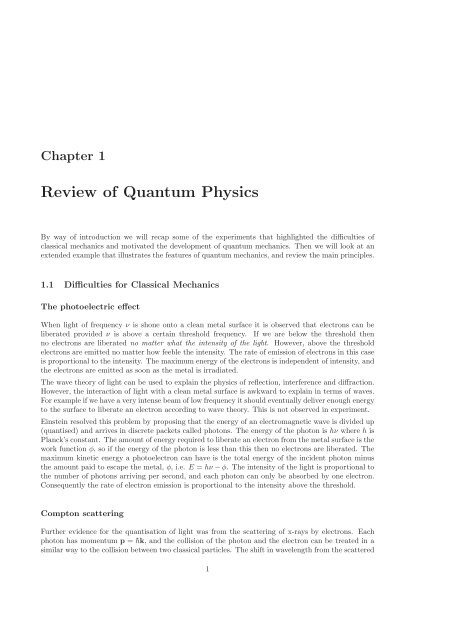
8 CHAPTER 1. REVIEW OF QUANTUM PHYSICSfrom the coefficients |c i | 2 = 1/2 for i = 1,3. The crucial part as we shall see later is that once thesystem has been measured in a particular state, it collapses into that eigenstate, so that any furthermeasurements recover the same result.Lastlywe could leavethis stateto evolve, which it will do accordingto the time dependent Schrödingerequation.ĤΨ = i¯h ∂ Ψ. (1.44)∂tAs we will see each of the energy eigenstates has a time varying factor of exp { −iE nt} ¯h , so we can writeΨ(x,t) = ∑ nc n φ n (x)e −iEnt/¯h . (1.45)In this example we have thatΨ(x,t) = √ 1√e −iE 0 t 2 πx¯h sin 2 a a + √ 1√e −9iE 0 t 2 3πx¯h sin 2 a a(1.46)P(x,t) = |Ψ(x,t)| 2 (1.47)= 1 (sin 2 πx 3πx+sin2a a a +2cos 8E )0t πx 3πxsin sin (1.48)¯h a awhere E 0 = ¯h2 n 2 π 22ma 2 . We plot the probability of finding the particle at a particular point x in thewell as a function of time P(x,t) = |Ψ(x,t)| 2 in Fig. 1.4. Note that the first two terms are justthe probability distributions for the n = 1 and n = 3 energy eigenstates, and the last term is the“interference” between these two states. This extended example illustrates most the main points ofthe postulates of quantum mechanics. We will discuss these, together with some better notation inthe next section.1.3 Dirac NotationThe notation of the last example was rather cumbersome. We had to repeatedly write down integralsigns in a long winded way. Dirac or bra-ket notation is a general, if slightly more abstract way ofwriting down the relevant equations. Essentially we denote the wave function by |Ψ〉, which is knownas a ket. Its complex conjugate is denoted by a bra 〈Ψ|. The integrals we encountered in the lastsection can be denoted: ∫φ ∗ (x)ψ(x)dx = 〈φ|ψ〉. (1.49)A compact notation for the energy eigenstates issimilarly if we take the conjugate of this we haveso the operator Ĥ can act to the left!VĤ|φ n 〉 = E n |φ n 〉, (1.50)〈φ n |Ĥ = E n〈φ n | (1.51)Often it is even more compact to label the eigenstate ket with simply the eigenvalue. For example ifwe consider the momentum operator:ˆp|p〉 = p|p〉 (1.52)

1.3. DIRAC NOTATION 9tP(x,t)=| ψ | 2xFigure 1.4: The time dependant probability distribution given in Eq. (1.48), for our particular initialstate.This equation (especially when read aloud!) may seem confusing, but the compactness afforded bythe notation is very useful for writing complicated expressions.We will see the real utility of this notation later when we discuss matrix mechanics, as it allows aunified of it with wave mechanics, and perturbation theory where the notation would otherwise bevery dense.From here onwards we will try use Dirac notation so that we become accustomed with it, but will notbe too formal.Analogy with vectorsThere is a strong analogy between Dirac notation, and vector notation. The table below illustratesthe analogies between the two different notations. If we use the matrix mechanics representation ofquantum physics, then this analogy becomes even stronger. However, this analogy is no coincidenceas they are both examples of linear vector spaces.

10 CHAPTER 1. REVIEW OF QUANTUM PHYSICSDirac NotationVector notationState |ψ〉 Vector aInner product 〈ψ|φ〉 Dot product a·bBasis states |ψ〉 = ∑ n c n|φ n 〉 Vector components a = a xˆx+a y ŷ+a z ẑOperators Ĥ|ψ〉 Matrices M·aOperator elements 〈φ|Ĥ|ψ〉 Matrix element H ij1.4 The PostulatesI The most complete knowledge we can have of the system is represented by the wave function|Ψ(t)〉.II Every observable O has a corresponding Hermitian operator Ô whose eigenvalues represent thepossible results of carrying out a measurement.III Eigenvalue, O i , with eigenstate |O i 〉 has a probability P = |〈O i |Ψ〉| 2 of being obtained from ameasurement of |Ψ〉.IV As a result of a measurement where the result O i is obtained the system collapses into state |O i 〉.V Between measurementsthe wavefunction |Ψ〉 evolves according tothe time-dependent Schrödingerequationi¯h ∂ |Ψ〉 = Ĥ|Ψ〉.∂tSome of the terminology in these postulates may seem unfamiliar to you. We will spend the next fewpages explaining what it means, and going over some of the methods used in the example at the startof this chapter.WavefunctionAswehavealreadystatedquantummechanicshasaprobabilisticinterpretation,andthewavefunctionis related to the probability density. Consequently we must make sure that the wavefunction isnormalised, or in Dirac notation∫〈Ψ|Ψ〉 = Ψ ∗ (x)Ψ(x)dx = 1. (1.53)VAn important feature of the Schrödinger equation is that it is a linear equation. Consequently if wehave two solutions |Ψ 1 〉 and |Ψ 2 〉 then we know that any linear combination of these two, |Ψ〉 is stilla solution|Ψ〉 = α|Ψ 1 〉+β|Ψ 2 〉 (1.54)where α,β may be any complex numbers.OperatorsAn operator converts a one mathematical function into another. In quantum mechanics we replacevariables by their corresponding operators. Some examples are given in the table below.

1.4. THE POSTULATES 11Classical VariablePosition xPosition vector rMomentum p xVector momentum pKinetic energy T = 1 2 mv2 = ˆp22mPotential energy V(r)Quantum Operatorˆx = xˆr = rˆp x = −i¯h ddxˆp = −i¯h∇ˆT = −¯h2 ∇ 2ˆV(r)Hamiltonian H = T +V Ĥ = −¯h2 ∇ 22m + ˆV(r)Energy E Ê = i¯h ∂ ∂tThe first important propertyof operatorscorrespondingto physicalobservablesis that they are linear,i.e.Ô(α|Ψ 1 〉+β|Ψ 2 〉) = αÔ|Ψ 1〉+βÔ|Ψ 2〉. (1.55)For example the differential operator d/dx is linear becauseddx (αf 1(x)+βf 2 (x)) = α df 1dx +βdf 2dxwhere as the operator “add a constant” f(x) → f(x)+c is not linear(αf 1 (x)+βf 2 (x))+c ≠ (α(f 1 (x)+c)+β(f 2 (x)+c)).2mHermitian OperatorsYou may have met the word Hermitian in the context of matrices. If we have a matrix denoted byH ij , where i denotes the row index, and j the column index, then its Hermitian conjugate is definedby H † ij = H∗ ji , that is we swap the rows and columns (transpose the matrix), and take the complexconjugate of each element. A matrix is said to be Hermitian if H † = H, that is if it is equal to itsHermitian conjugate.Here we define the Hermitian conjugate as follows∫〈φ|Ô|ψ〉 = φ ∗ Ôψdx (1.56)∫⇒ 〈φ|Ô|ψ〉† = 〈ψ|Ô|φ〉∗ = ψÔ∗ φ ∗ dx (1.57)i.e. we havesimply swappedaroundφand ψ and takenthe complex conjugateofthe operator. We canshow that all physical observables are Hermitian operators (i.e. equal to their Hermitian conjugate)〈φ|Ô|ψ〉 = 〈φ|Ô|ψ〉† . As an example consider the momentum operator ˆp = −i¯h ddx(∫ ∞〈φ|ˆp|ψ〉 = φ ∗ (x)(−i¯h) d )−∞ dx ψ(x)dx integrate by parts ↓ (1.58)= [φ ∗ (x)(−i¯h)ψ(x)] ∞ −∞} {{ }=0 as φ(±∞)=ψ(±∞)=0+∫ ∞−∞ψ(x)(i¯h) ddx φ∗ (x)dx (1.59)(∫ ∞= ψ ∗ (x)(−i¯h) d ) ∗−∞ dx φ(x) (1.60)= 〈φ|ˆp|ψ〉 † (1.61)

12 CHAPTER 1. REVIEW OF QUANTUM PHYSICSi.e. the operator ˆp is Hermitian.An important property of Hermitian operators is that they have real eigenvalues, and orthogonaleigenstates (or eigenstates that can be made orthogonal). We can prove this important result byconsidering an operator  with eigenstates defined by Â|a n〉 = a n |a n 〉. If we write down this equationand its Hermitian conjugate we haveIf we equate these two objects thenÂ|a n 〉 = a n |a n 〉 ⇒ 〈a m |Â|a n〉 = a n 〈a m |a n 〉 (1.62)〈a m | = a∗ m〈a m | ⇒ 〈a m |Â|a n〉 = a ∗ m〈a m |a n 〉 (1.63)(a ∗ m −a n )〈a m |a n 〉 = 0. (1.64)Now we assume here that all the eigenvalues are different. We also know that 〈a m |a m 〉 ̸= 0.n ≠ m ⇒ a ∗ m ≠ a n so 〈a m |a n 〉 = 0 i.e. orthogonal eigenstates (1.65)n = m ⇒ a ∗ m = a m i.e. eigenvalues must be real (1.66)If we have time we will return to the case where the eigenvalues are not distinct when we come todegenerate perturbation theory. Here we will show that even in this case it is possible to constructeigenstates that are orthogonal.ExpectationThe expectation value of an operator Ô for a state |Ψ〉 is defined by∫〈Ô〉 = 〈Ψ|Ô|Ψ〉 = ∗Ψ (x)ÔΨ(x)dx. (1.67)Note that the wavefunctionshere mustbe normalised, otherwisewe shoulduse the modified expressionV〈Ψ|Ô|Ψ〉〈Ô〉 =〈Ψ|Ψ〉(1.68)Expansion in terms of eigenstatesOnce we have calculated the set of eigenstates of an operator, then we can use these states to expressan arbitrary state. The crucial feature of this expansion is the orthogonality of the eigenstates,and their normalisation (orthonormality). For an operator  we have already found its eigenstatesÂ|a n 〉 = a n |a n 〉. An arbitrary state |Ψ〉 can then be written|Ψ〉 = ∑ nc n |a n 〉, (1.69)where c n are the constant coefficients in the expansion. The eigenstates (of an Hermitian operator)are referred to as a complete set as we can represent any other state in this space as a sum over theeigenstates. A typical example of this is a Fourier series, that you have met in the context of a squarewell. There we have (depending on the boundary conditions used)Ψ(x) = ∑ (A n sin nπxa +B ncos nπx )(1.70)an

1.4. THE POSTULATES 13so here A n and B n are the expansion coefficients and the cos and sin the eigenstates.We can use the power of Dirac notation to work out the expectation of the operator  of the wavefunction|Ψ〉〈Â〉 = 〈Ψ|Â|Ψ〉 = ∑ n〈a n |c ∗ nÂ∑ mc m |a m 〉 (1.71)= ∑ n,mc ∗ nc m 〈a n |Â|a m〉 = ∑ } {{ }n,mc ∗ nc m a m 〈a n |a m 〉 (1.72)} {{ }a m|a m〉δ nm= ∑ c ∗ nc m a m δ nm = ∑n,mn|c n | 2 a n . (1.73)So |c n | 2 is the probability of measuring eigenvalue a n , and our expectation value is just a sum withthe appropriate weights.The weights c n can be worked out again by using orthonormality〈a m |×|Ψ〉 = 〈a m |× ∑ nc n |a n 〉 (1.74)〈a m |Ψ〉 = ∑ nc n 〈a m |a n 〉} {{ }= c m . (1.75)δ nmNote that this definition of c m = 〈a m |Ψ〉 leads to an important identityΨ = ∑ nc n |a n 〉 = ∑ n|a n 〉〈a n |Ψ〉 (1.76)⇒ 1 = ∑ n|a n 〉〈a n |. (1.77)This result known as the resolution of the identity is often useful in quantum mechanics, though wewill not refer to it further in this course.The above results have implicitly assumed that the spectrum of eigenvalues is discrete, as we see inthe energy spectra of bound states. Free particles have a continuum of possible energy values, butnone the less the above results can be translated so that they hold there. In this course we will mainlyfocus on operators that have a discrete set of energy eigenvalues, so will not discuss this further.Compatible and incompatible observablesIf we have two observables corresponding to the operators  and ˆB then we can calculate the eigenstatesof each operatorÂ|a n 〉 = a n |a n 〉 (1.78)ˆB|b n 〉 = b n |b n 〉. (1.79)Now suppose we perform a measurement corresponding to Â. The system will then collapse into oneof the eigenstates of Â, say |a 1〉. If we then measure using ˆB the system will collapseinto an eigenstateof ˆB corresponding to the value measured, say |b 1 〉.• If the eigenstate |a 1 〉 and |b 1 〉 are the same, then we say that the two observables are compatible.• If the two eigenstates are different then we say that the two observables are incompatible.

14 CHAPTER 1. REVIEW OF QUANTUM PHYSICSIf two observables are compatible then the share eigenstates |a n 〉 = |b n 〉. ConsequentlyˆBÂ|a n〉 = ˆBa n |a n 〉 = a n b n |a n 〉 (1.80)ˆB|b n 〉 = Âb n|a n 〉 = a n b n |b n 〉 (1.81)⇒ (ˆB − ˆBÂ)|a n〉 = 0. (1.82)This is true for all eigenstates, so we knowthat compatible observablesmust commute! The commutatorof two observables is defined by [Â, ˆB] = ˆB− ˆBÂ, and plays a central role in quantum mechanics.Note the converse is true: if we have two observables that commute then they are compatible[Â, ˆB]|Ψ〉 = 0 (1.83)⇒ ˆB|b n 〉 = ˆBÂ|b n〉 = Âb n|b n 〉 (1.84)⇒ ˆB(Â|b n〉) = b n (Â|b n〉) (1.85)⇒ Â|b n〉 ∝ |b n 〉 i.e. |b n 〉 are  eigenstates! (1.86)We have proven that if  and ˆB commute then the are compatible.If we have two incompatible (i.e. non-commuting) observables  and ˆB, and we alternate in theirmeasurement, then we repeatedly change the state that the system is in. They lie at the heart of theuncertainty relation in quantum mechanics.Generalised Uncertainty RelationWe define the deviation of an operator from its mean value by d = Â−Ā. (1.87)The uncertainty of  is then (∆A)2 = 〈Â2 d 〉 = 〈Â2 〉−Ā2 , and similarly for B. For an arbitrary state|Ψ〉 we consider the state|Φ〉 = (Âd +iλˆB d )|Ψ〉. (1.88)If we calculate 〈Φ|Φ〉 ≥ 0 we find〈Ψ|(Âd −iλˆB d )(Âd +iλˆB d )|Ψ〉 = (∆A) 2 +λ 2 (∆B) 2 +λ〈i[Âd, ˆB d ]〉. (1.89)This is true for all λ. We can minimise over λ to get the best bound, soNow since Ā and ¯B are just numbers, they must commute so〈i[Âd, ˆB d ]〉 2 −4(∆A) 2 (∆B) 2 ≤ 0. (1.90)∆A∆B ≥ 1 2 |〈i[Â, ˆB]〉| (1.91)As an example of this consider A = x and B = p. Their commutator is given byso we have ∆x∆p ≥ 1 2¯h.[ˆx, ˆp]ψ = x(−i¯h) ddx ψ +i¯h d (xψ) = i¯hψ (1.92)dx

1.4. THE POSTULATES 15Labelling quantum statesWe have seen that a convenient way to identify an eigenstate of an operator is to label it withthe corresponding eigenvalues of the operator. In the case of the square well we chose to label theeigenstates with their energy eigenvalues that can be calculated from the Hamiltonian operator Ĥ.This provides us with a quantum number that labels each state. However it may happen that anoperator is degenerate, i.e. has two or more states with the same eigenvalue. We have to be carefulin labelling states like this, as we will now discuss.Suppose we have an operator  whose eigenvalues we use to label our quantum states. Suppose thisoperator has some degenerate states, as discussed above. We must then find a second operator ˆBthat commutes with  (i.e. is compatible), but does not suffer from identical degeneracies. We canthen use this operator to distinguish between the degenerate states of Â. It may happen that  andˆB some degeneracies in common, in which case we must find a third compatible operator Ĉ withwhich to disginguish the degenerate states. We continue this process until we have a complete set ofcommuting observables so we can use their quantum numbers to uniquely label every eigenstate. Anexample of this is illustrated in the table below. ˆB Ĉ0 0 01 0 01 1 01 1 12 0 02 1 02 1 12 2 0......First we try and label the states using the eigenvalues of operator Â, but some states have the samelabel. We then find a commuting operator ˆB and try and label all the states. This helps us uniquelyidentify most states, but there are still some degenerate states, so we have to find a third operator Ĉthat commutes with the previous two so we can uniquely identify the states. In this case we need 3quantum numbers to uniquely identify a state.The Schrödinger equationOne way to “derive” the Schrödinger equation is as follows. Suppose we have a system with a classicalenergy E given byE = p2+V(x), (1.93)2mwhere as usual p is the momentum, V(x) the potential, and m the mass. We simply replace eachof the classical quantities by their corresponding operators as discussed earlier, and multiply by thewave function( ) ˆp2Ê|Ψ〉 =2m + ˆV(x) |Ψ〉 (1.94)⇒ i¯h ∂ (∂t |Ψ〉 = − ¯h2 ∂ 2 )2m∂x 2 +V(x) |Ψ〉 (1.95)

16 CHAPTER 1. REVIEW OF QUANTUM PHYSICS⇒ i¯h ∂ |Ψ〉 = Ĥ|Ψ〉. (1.96)∂tFrom this equation we can calculate the time-independent states by assuming that the wavefunctionis of the form |Ψ(x,t)〉 = ψ(x)T(t).1(− ¯h2 d 2 )ψ 2mdx 2ψ +Vψ = i¯h 1 T} {{ }Only depends on xdTdt} {{ }Only depends on t= E (1.97)each side can only be a constant which we call E. We thus have two equations) (− ¯h22m ∇2 +V ψ = Eψ ⇒ Ĥψ = Eψ (1.98)E = i¯h 1 dTT dt ⇒ T = e−iEt/¯h . (1.99)The first of these is the time-independent Schrödinger equation, and the second tell us how stationarystates depend on time. We can substitute this result into our expansion, as we did in the example atthe start of this chapterΨ = ∑ c n ψ n e −iEnt/¯h .n(1.100)Time dependence of expectation valuesHow does the expectation value of a variable change with time?∂∂t 〈Â〉 = ∂ 〈Ψ|Â|Ψ〉 (1.101)∂t( ) ( )∂ ∂=∂t 〈Ψ| Â|Ψ〉+〈Ψ|Â∂t |Ψ〉 (1.102)} {{ } } {{ }−i¯h ∂ ∂t 〈Ψ|=〈Ψ|Ĥ i¯h ∂ ∂t |Ψ〉=Ĥ|Ψ〉= 1 ) (〈Ψ|ÂĤ i¯h−ĤÂ|Ψ〉 (1.103)= ī 〈[Ĥ,Â]〉 (1.104)hFor comparison we compare this rather compact derivation in Dirac notation to the longer derivationin conventional notation∂〈Â〉 = ∂ ∫Ψ ∗ ÂΨdx (1.105)∂t ∂t∫∂Ψ ∗= ÂΨ+Ψ ∗  ∂Ψ dx (1.106)}{{}∂t}{{}∂tΨ ∗Ĥ=−i¯h∂Ψ∗ ∂tĤΨ=i¯h ∂Ψ∂t∫ −1=i¯h Ψ∗ĤÂΨ+Ψ∗  1(1.107)i¯hĤΨdx= ī ∫Ψ ∗( )ĤÂ−ÂĤ Ψdx (1.108)h= ī 〈[Ĥ,Â]〉 (1.109)h

1.5. PROBLEMS 17Thus if  commutes with Ĥ then we have a conserved quantity. As you know conserved quantitiesplay a crucial role in mechanics. There is also a very deep connection between conserved quantitiesand symmetries of a system (Noether’s theorem), but this is beyond the scope of this course.1.5 ProblemsIf you are short of time, then focus on the following problems: 2, 3, 4, 6, 12, 13, 16, 171A. Withoutcalculation,sketchthewavefunctionoftheexcitedstatewithenergyE 4 forthepotentialwell shown in the figure . Label the important features of your sketch.E 4(hint: the wavefunctionshould decayin the forbidden regionswhere V > E 4 , and oscillateinsidethe well).2A. (i) Observables are represented by linear operators. What is meant by linear?(ii) Two state functions are orthogonal. What is meant by orthogonal?(iii) Functions ψ n form a complete set. What is meant by a complete set?3A. Write down the operators corresponding to the following observables(i) The position along the x axis(ii) The momentum in the x direction(iii) The momentum in the y direction(iv) The total momentum(v) The total momentum squared(vi) The kinetic energy for a particle confined to the x axis(vii) The kinetic energy for motion in three dimensions.(viii) The potential energy(ix) The total energy for a particle confined to the x axis(x) The total energy for a particle in three dimensions4A. Expand the Dirac notation to prove the following (note c is a complex number).(i) 〈ψ 1 |cψ 2 〉 = c〈ψ 1 |ψ 2 〉(ii) 〈cψ 1 |ψ 2 〉 = c ∗ 〈ψ 1 |ψ 2 〉(iii) 〈ψ 3 |ψ 1 +ψ 2 〉 = 〈ψ 3 |ψ 1 〉+〈ψ 3 |ψ 2 〉(iv) If the wave function ψ can be written as the sum of orthogonal functions ψ n , show that〈ψ n |ψ〉 = c n where c n is the corresponding expansion coefficient of ψ.

18 CHAPTER 1. REVIEW OF QUANTUM PHYSICS5A. |φ 1 〉 and |φ 2 〉 are normalised eigenfunctions of observable Â. However they are degenerate (havethe same eigenvalue of Â) so are not necessarily orthogonal. If 〈φ 1 |φ 2 〉 = c and c is real, findlinear combinations of φ 1 and φ 2 which are normalised and orthogonal toa) φ 1b) φ 1 +φ 26B. The operators Â1 to Â6 are defined as follows 1 ψ(x) = ψ 2 (x) 2 ψ(x) = dψ(x)dx 3 ψ(x) = i dψ(x)dx 4 ψ(x) = x 2 ψ(x) 5 ψ(x) = sinψ(x) 6 ψ(x) = d2 ψ(x)dx 2where you may assume that ψ(x) is defined over the range −∞ < x < ∞ and that ψ(x) and itsderivative vanish at these limits.Which of these operators are linear? Which are Hermitian?What the eigenfunctions for the linear Hermition operators?7B. A particle in the ground state (n = 1) of a 1D potential well extending from 0 ≤ x ≤ a can bedescribed by the wave function ψ 1 (x) = Asin(πx/a). A particle in the n = 2 state of the sameinfinite potential well has the wavefunction ψ 2 (x) = Bsin(2πx/a)(i) State the normalisation condition satisfied by ψ 1 (x).√2(ii) Show that A =a .(iii) Find B.(iv) What is the probility of finding the particle at x = a/2?(v) Show that ψ 1 (x) = ψ 1 (a−x). What is the name of this type of function?(vi) Show that ψ 2 (x) = −ψ(a−x). What is the name given to this type of function?(vii) Determine the probability that a particle in the n = 1 state resides between x = 0 andx = a/4.(viii) Determine the probability that a particle in the n = 2 state resides between x = 0 andx = a/4(ix) A superposition of the two states is also a possible state i.e. ψ = c 1 ψ 1 +c 2 ψ 2 . Show that|c 1 | 2 +|c 2 | 2 = 1.8B. Determine the normalising constants for the following wavefunctions(i) ψ(x) = A 1 sin(πx/a); 0 ≤ x ≤ a(ii) ψ(x,y,z) = A 2 sin(πx/a)sin(πy/b)sin(πz/c); 0 ≤ x ≤ a, 0 ≤ y ≤ b, 0 ≤ z ≤ c(iii) ψ(r) = A 3 e −r/a ; for a sphere of infinite radius

1.5. PROBLEMS 199B. A particle is represented by the wavefunctionψ(x) = Axe −αx2Calculate ∆x and ∆p x by making use of the momentum operator. Hence show that ∆x∆p x =3¯h/210B. Show that in one dimension the following wavefunctions are orthogonal ψ 1 = e −x2 , ψ 2 = xe −x2and ψ 3 = (2x 2 −1)e −x2 . How could you make them orthonormal?11B. Which of the following operators are Hermitian, given that  and ˆB are Hermitian?Â+ ˆB,cÂ,ˆB,ˆB + ˆBÂShow that in one dimension, for functions that tend to zero at x = ±∞, the operator ∂/∂x isno Hermitian, but the following operator is −i¯h∂/∂x. Is the operator ∂ 2 /∂x 2 Hermitian?12B. The two operators  and ˆB represent physical observables.(i) Write out the commutation relation [Â, ˆB] in terms of  and ˆB(ii) If  and ˆB “commute”, state the relation satisfied by  and ˆB and explain the physicalsignificance of this result.(iii) What can be said about the eigenfunctions of  and ˆB if these operators commute?(iv) If  and ˆB do not commute, what is the physical significance of this result?(v) What can be said about the eigenfunctions of  and ˆB if these operators do not commute?13C. Observable  has eigenfunctions ψ 1 and ψ 2 with eigenvalues of a 1 and a 2 . Observable ˆB haseigenfunctions χ 1 and χ 2 with eigenvalues b 1 and b 2 . The eigenfunctions can be related asfollowsχ 1 = (2ψ 1 +3ψ 2 )/ √ 13χ 2 = (3ψ 1 −2ψ 2 )/ √ 13ˆB is measured and a value of b 1 is obtained. If  were now to be measured, what would be theprobabilities of getting a 1 and a 2 in this measurement? If  is now indeed measured, and thenˆB measured again, show that the probability of getting b 1 again is 97/16914C. For a certain type of atom the observable  has eigenvalues ±1, with corresponding eigenfunctionsu + and u − . Another observable ˆB also has eigenvalues of ±1, but correspondingeigenfunctions are ν + and ν − . The eigenfunctions are related byν + = (u + +u − )/ √ 2ν − = (u + −u − )/ √ 2Show that Ĉ ≡ Â+ ˆB is an observable and find the possible results of a measurement of Ĉ.Find the probability of obtaining each result when a measurement of Ĉ is performed on an atomin the state u + , and the corresponding state of the atom immediately after the measurement interms of u + and u − .

20 CHAPTER 1. REVIEW OF QUANTUM PHYSICS15B. What is the definition of the commutator [Â, ˆB]?Prove the following commutation relations(i) [ˆp x , ˆp y ] = 0(ii) [ˆp 2 , ˆp x ] = 0(iii) [ˆp x ,Ĥ] = −i¯h∂V∂x(iv) [Ĥ,ˆx] = −i¯h mˆp x16B. In a certain system, Â has eigenvalues a 1 and a 2 corresponding to eigenfunctionsψ 1 = (u 1 +u 2 )/ √ 2 (1.110)ψ 2 = (u 1 −u 2 )/ √ 2, (1.111)where u 1 and u 2 are stationary states with energies E 1 and E 2 . Â is measured and found tohave value a 1 . Find how 〈Â〉 varies with time subsequently17B. (i) State the time-dependent Schrödinger equation.(ii) The time-independent wave function for a 1D system ψ(x) can be expressed in terms of acomplete set of energy eigenfunctions ψ n (x) with corresponding eigenvalues E nψ(x) = ∑ nc n ψ n (x).How can the the time-dependent wavefunction, Ψ(x,t) be expressed in terms of the energyeigenfunctions?(iii) Using your result from part (ii), show that Ψ(x,0), the state of the system at t = 0 isequivalent to the expression for ψ(x) quoted in (ii).

1.6. ANSWERS TO CHAPTER 1 PROBLEMS 211.6 Answers to Chapter 1 Problems1. Oscillating wavefunction where E > V, decaying wavefunction in forbidden regions E < V.2. (i) Linear operators obey Â(af 1(x)+bf 2 (x)) = aÂf 1(x)+bÂf 2(x)(ii) Orthogonal functions obey ∫ ba f 1(x) ∗ f 2 (x)dx = 0 for a particular range (a,b)(iii) Any arbitrary function ψ can be written as a unique sum of a complete set of functionsψ n : ψ = ∑ n c nψ n3. (i) ˆx = x(ii) ˆp x = −i¯h ddx(iii) ˆp y = −i¯h ddy(iv) ˆP = −i¯h∇(v) ˆP 2 = −¯h 2 ∇ 2(vi) ˆT = ˆp2 x2m = − ¯h22md 2dx 2(vii) ˆT = ˆP 22m = − ¯h22m ∇2(viii) ˆV = V(x)(ix) Ĥ = ˆT + ˆV = − ¯h22m dx+V(x) 2d 2(x) Ĥ = ˆT + ˆV = − ¯h22m ∇2 +V(x)4. (i) 〈ψ 1 |cψ 2 〉 = ∫ dxψ ∗ 1cψ 2 = c〈ψ 1 |ψ 2 〉(ii) 〈cψ 1 |ψ 2 〉 = ∫ dx(cψ 1 ) ∗ ψ 2 = c ∗ 〈ψ 1 |ψ 2 〉(iii) 〈ψ 3 |ψ 1 +ψ 2 〉 = ∫ dxψ ∗ 3 (ψ 1 +ψ 2 ) = 〈ψ 3 |ψ 1 〉+〈ψ 3 |ψ 2 〉(iv)ψ = ∑ nc n ψ n5. (a) If ψ = 1 √1−c 2 (−cφ 1 +φ 2 ) then 〈ψ|φ 1 〉 = 0(b) If ψ = 1 √ 2−2c(φ 1 −φ 2 ) then 〈ψ|φ 1 +φ 2 〉 = 0⇒ 〈ψ m |ψ〉 = ∑ c n 〈ψ m |ψ n 〉} {{ }nδ mn⇒ c m = 〈ψ m |ψ〉6. Linear:  2 ,Â3,Â4,Â6Hermitian:  3 ,Â4,Â6Eigenfunctions (Âψ = λψ): 3 : ψ(x) = e −iλx 4 : ψ(x) = δ(x−x 0 ) 4 : ψ(x) = Ae √ λx +Be −√ λx