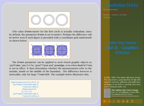
3.2. Inside, outside or in the middle?When we draw a double boundary for an object, one natural question iswhether the dimensions of the object are <strong>with</strong> reference to the outer orinner boundary. For example, if we specify the radius of a circle as 1 cmand give it a double border, is it the inner circle or the outer circle that hasradius 1 cm? By default, it’s the outer circle, but it can be changed <strong>with</strong> thehelp of the dimen parameter. Its possible values are inner, middle andouter and the default value is outer. The example below illustrates this:\begin{pspicture}(0,0)(2,2)\pscircle[doubleline=true,%doublesep=5pt,%dimen=outer]%(1,1){1}\end{pspicture}\hspace{.5cm}\begin{pspicture}(0,0)(2,2)\pscircle[doubleline=true,%doublesep=5pt,%dimen=middle]%(1,1){1}\end{pspicture}\hspace{.5cm}\begin{pspicture}(0,0)(2,2)\pscircle[doubleline=true,%doublesep=5pt,%dimen=inner]%(1,1){1}\end{pspicture}givesBorderline TricksDouble boundaryInside, outside or in the middle?Borders—visible or invisibleShadowsOnline L A T E X TutorialPart II – Graphics<strong>PSTric</strong>ksc○2002, 2003, The Indian T E X Users GroupThis document is generated by PDFT E X <strong>with</strong>hyperref, pstricks, pdftricks and pdfscreenpackages on an intel PC running GNU/LINUXand is released under LPPLThe Indian T E X Users GroupFloor iii, sjp Buildings, Cotton HillsTrivandrum 695014, indiahttp://www.tug.org.in£ ¡ ¢ ¤ ¥ ¦ © 8/19
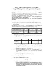
Borderline TricksDouble boundaryInside, outside or in the middle?Borders—visible or invisibleShadows(The value dimen=outer for the first circle is actually redundant, sinceby default, the parameter dimen is set to outer). Perhaps the difference willbe better seen if each figure is provided <strong>with</strong> a coordinate grid underneathas shown below:21210000 1 2 0 1 2 0 1 221Online L A T E X TutorialPart II – Graphics<strong>PSTric</strong>ksThe dimen parameter can be applied to such closed graphic objects as\psframe, \pscircle, \psellipse and \pswedge, even when doublelinesis not in effect. It then determines whether the measurements refer to theoutside, inside or the middle of the boundary. The difference however isnoticeable, only for large linewidth. The example below illustrates this.\begin{pspicture}(0,0)(5,5)\psframe[linewidth=2mm,%linecolor=Red,%dimen=outer]%(1,1)(2,2)\psframe[linewidth=2mm,%linecolor=Blue,%c○2002, 2003, The Indian T E X Users GroupThis document is generated by PDFT E X <strong>with</strong>hyperref, pstricks, pdftricks and pdfscreenpackages on an intel PC running GNU/LINUXand is released under LPPLThe Indian T E X Users GroupFloor iii, sjp Buildings, Cotton HillsTrivandrum 695014, indiahttp://www.tug.org.in£ ¡ ¢ ¤ ¥ ¦ © 9/19
- Page 1 and 2:
Graphics with PSTricksGetting the p
- Page 3 and 4:
1.1. Getting the pointsAny picture
- Page 5 and 6:
Graphics with PSTricksThe PSTricks
- Page 7 and 8:
Graphics with PSTricksillustrated i
- Page 9 and 10:
Graphics with PSTricks\begin{pspict
- Page 11 and 12: Graphics with PSTricks\begin{pspict
- Page 13 and 14: Graphics with PSTricks100 1 2In thi
- Page 15 and 16: 1.4. Ends of LinesLines can be prov
- Page 17 and 18: Graphics with PSTricks\begin{pspict
- Page 19 and 20: parameter value descriptiondotsize
- Page 21 and 22: Graphics with PSTricksThe default v
- Page 23 and 24: 1.5. Bent Lines and PolygonsAs in t
- Page 25 and 26: “filled up” polygon. For exampl
- Page 27 and 28: Graphics with PSTricksGetting the p
- Page 29 and 30: 1.6. Simple CurvesCircles, ellipses
- Page 31 and 32: 321030 ◦ 60 ◦Graphics with PSTr
- Page 33 and 34: Graphics with PSTricksGetting the p
- Page 35 and 36: Graphics with PSTricksAnother curve
- Page 37 and 38: Ordinary colorsMore colorsFill—in
- Page 39 and 40: Colorful TricksOrdinary colorsMore
- Page 41 and 42: \begin{pspicture}(0,0)(3,3)\psframe
- Page 43 and 44: NAME CMYK COLOR NAME CMYK COLORGree
- Page 45 and 46: \begin{pspicture}(0,0)(4,4)\psframe
- Page 47 and 48: 2.4. Custom colorsIf you are not sa
- Page 49 and 50: 2.5. From one color to anotherThere
- Page 51 and 52: \begin{center}\definecolor{myblue}{
- Page 53 and 54: \pscircle[linestyle=none,%linewidth
- Page 55 and 56: Borderline TricksDouble boundaryIns
- Page 57 and 58: 3.1. Double boundaryIn the first ch
- Page 59 and 60: doublesep=5pt,%doublecolor=Blue]%(1
- Page 61: \begin{pspicture}(0,0)(4,2)\psframe
- Page 65 and 66: 3.3. Borders—visible or invisible
- Page 67 and 68: \begin{pspicture}(0,0)(3,3)\psframe
- Page 69 and 70: 3.4. ShadowsAn object can be given
- Page 71: \begin{pspicture}(0,0)(3.5,3.5)\psp
- Page 77 and 78: A “closed” curve joining specif
- Page 79 and 80: 4.2. Invisible endsthere’s a thir
- Page 81 and 82: Curvy Tricks543543Open and closed c
- Page 83 and 84: Curvy Tricks55Open and closed curve
- Page 85 and 86: value of 0 for the third number in
- Page 87 and 88: Curvy Tricks4.4. A new curveAnother
- Page 89 and 90: This point, which we denote by z 12
- Page 91 and 92: 5. More on CoordinatesCoordinate gr
- Page 93 and 94: example:\psgrid(2,3)(1,2)(5,4)431 2
- Page 95 and 96: More on Coordinatesparameter meanin
- Page 97 and 98: Instead of scaling by the same amou
- Page 99 and 100: 5.3. Another type of coordinatesThe
- Page 101 and 102: \definecolor{PaleApricot}{cmyk}{0,0
- Page 103 and 104: \begin{pspicture}(0,-0.5)(6,3.5)\Sp
- Page 105 and 106: such that the required point has x-
- Page 107 and 108: 5.5. Changing the systemIn drawing
- Page 109 and 110: \begin{pspicture}(0,0)(4,4)\pspolyg
- Page 111 and 112: Appendix—Math in PostScriptWe’v
- Page 113 and 114:
Placing ThingsPlacing and rotating
- Page 115 and 116:
Placing Things6.1. Placing and rota
- Page 117 and 118:
Placing Things\begin{pspicture}(0,1
- Page 119 and 120:
Placing Things98Placing and rotatin
- Page 121 and 122:
BASELINEheightwidthbydepthBASELINEP
- Page 123 and 124:
Placing ThingsFor vertically shifti
- Page 125 and 126:
Placing Things\definecolor{PaleApri
- Page 127 and 128:
Placing Thingsangle letter meaning
- Page 129 and 130:
Placing ThingsCPlacing and rotating
- Page 131 and 132:
We show below The positions of the
- Page 133 and 134:
Placing Things\begin{pspicture}(-4,
- Page 135 and 136:
Plotting TricksFunction plottingAxe
- Page 137 and 138:
7.1. Function plottingFor a mathema
- Page 139 and 140:
Plotting Tricks\begin{pspicture}(-2
- Page 141 and 142:
Plotting Tricks\psset{unit=0.5}\beg
- Page 143 and 144:
7.2. Axes of coordinatesOften in ma
- Page 145 and 146:
Plotting Tricks323(3,2)•Function
- Page 147 and 148:
We have included a background grid
- Page 149 and 150:
Plotting Tricks\begin{pspicture}(-2
- Page 151 and 152:
\begin{pspicture}(-3,-3)(3,3)\psaxe
- Page 153 and 154:
Plotting Tricks\begin{pspicture}(-3
- Page 155 and 156:
Note that the entries in the first
- Page 157 and 158:
Plotting Tricks\psset{unit=0.66}\re
- Page 159 and 160:
7.3. Data plottingThe command \pspl
- Page 161 and 162:
Plotting Tricks\begin{pspicture}(0,
- Page 163 and 164:
The last command we describe for da
- Page 165 and 166:
Plotting Tricks\savedata{\dirdata}[
- Page 167 and 168:
Simple customizationHigher level cu
- Page 169 and 170:
we can use \colgrid every time we n
- Page 171 and 172:
8.2. Higher level customizationApar
- Page 173 and 174:
Let’s now take a closer look at t
- Page 175 and 176:
this is the state we are in:Custom
- Page 177 and 178:
Custom Graphics\psset{unit=1.5cm}\b
- Page 179 and 180:
treating the current point as the f
- Page 181 and 182:
Custom Graphics\begin{pspicture}(-2
- Page 183 and 184:
Custom Graphics\begin{pspicture}(0,
- Page 185 and 186:
Custom Graphics\renewcommand{\pshla
- Page 187 and 188:
Custom Graphics\begin{pspicture}(0,