Background Subtraction Using Ensembles of Classifiers with an ...

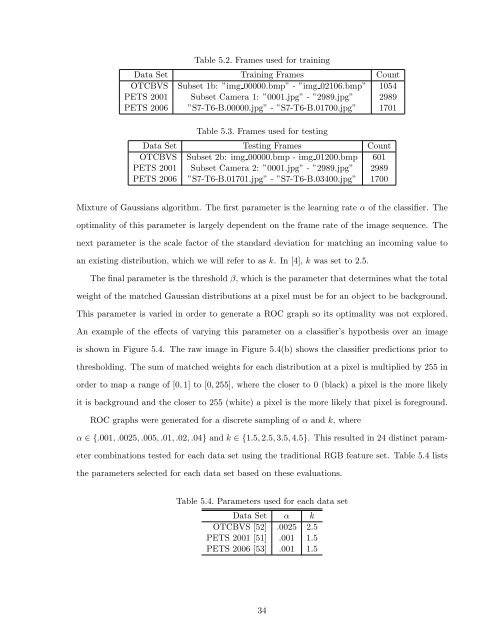
Table 5.2. Frames used for trainingData Set Training Frames CountOTCBVS Subset 1b: ”img 00000.bmp” - ”img 02106.bmp” 1054PETS 2001 Subset Camera 1: ”0001.jpg” - ”2989.jpg” 2989PETS 2006 ”S7-T6-B.00000.jpg” - ”S7-T6-B.01700.jpg” 1701Table 5.3. Frames used for testingData Set Testing Frames CountOTCBVS Subset 2b: img 00000.bmp - img 01200.bmp 601PETS 2001 Subset Camera 2: ”0001.jpg” - ”2989.jpg” 2989PETS 2006 ”S7-T6-B.01701.jpg” - ”S7-T6-B.03400.jpg” 1700Mixture of Gaussians algorithm. The first parameter is the learning rate α of the classifier. Theoptimality of this parameter is largely dependent on the frame rate of the image sequence. Thenext parameter is the scale factor of the standard deviation for matching an incoming value toan existing distribution, which we will refer to as k. In [4], k was set to 2.5.The final parameter is the threshold β, which is the parameter that determines what the totalweight of the matched Gaussian distributions at a pixel must be for an object to be background.This parameter is varied in order to generate a ROC graph so its optimality was not explored.An example of the effects of varying this parameter on a classifier’s hypothesis over an imageis shown in Figure 5.4. The raw image in Figure 5.4(b) shows the classifier predictions prior tothresholding. The sum of matched weights for each distribution at a pixel is multiplied by 255 inorder to map a range of [0, 1] to [0, 255], where the closer to 0 (black) a pixel is the more likelyit is background and the closer to 255 (white) a pixel is the more likely that pixel is foreground.ROC graphs were generated for a discrete sampling of α and k, whereα ∈ {.001, .0025, .005, .01, .02, .04} and k ∈ {1.5, 2.5, 3.5, 4.5}. This resulted in 24 distinct parametercombinations tested for each data set using the traditional RGB feature set. Table 5.4 liststhe parameters selected for each data set based on these evaluations.Table 5.4. Parameters used for each data setData Set α kOTCBVS [52] .0025 2.5PETS 2001 [51] .001 1.5PETS 2006 [53] .001 1.534