Stochastic Simulation in Timberland Investment Analysis - sofew

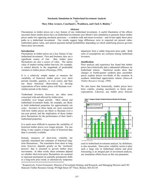
Stochastic Simulation in Timberland Investment AnalysisbyMary Ellen Aronow, Courtland L. Washburn, and Clark S. Binkley 1AbstractFluctuations in timber prices are a key feature of any timberland investment. A useful illustration of the effectsuncertain future timber prices have on timberland investments uses Monte Carlo simulation to generate future timberprices under two opposing stochastic processes – a random walk and mean reversion – and in-turn apply these pricepaths to a timberland investment. Our results suggest large differences exist in expected net present value,timberland option value, and interest payment default probabilities depending on which underlying process governsfuture price movements.IntroductionFluctuations in timber prices are a key feature of anytimberland investment. First and foremost, they are asignificant source of risk. But, timber pricefluctuations are also a source of value. The optionvalue of market timing timber harvests, for example,is related directly to the magnitude of predictablevariation in timber prices (Plantinga,1998).It is a relatively simple matter to measure thevariability of historical timber prices over shortperiods (months, quarters, or even years), and thenuse these historical observations to developexpectations of how timber prices will fluctuate oversimilar periods in the future.Timberland investors, however, are often moreconcerned with and affected by timber pricevariability over longer periods. Most closed endtimberland investment funds, for example, are likelyto hold timberland properties for approximately tenyears. Investors in these funds are most concernedwith how timber prices are likely to fluctuate over aten-year period, and the implication of those timberprice fluctuations for the performance of their fund’stimberland properties.It is much more difficult to measure the variability ofhistorical timber prices over longer periods. For onething, it may require a longer series of historical datathan is currently available.Instead, measures of short-term volatility aretypically translated into estimates of historical longtermfluctuations. The translation from short to longterm, however, depends greatly on the ‘stochasticprocess’ that is assumed to govern timber pricemovements. In other words, these estimates dependon whether short-term price fluctuations are assumedto represent permanent (or partially permanent) shiftsin a long-term price trend, or alternatively temporarydepartures from a stable long-term price path. Bothsorts of assumptions are common among timberlandinvestors.JustificationPrior analysis and experience has found that timberprices have historically had a substantial influence ontimberland returns. Statistical results show thatchanges in fourth-quarter southern pine sawtimberprices explain almost two-thirds of the variation insouthern timberland appreciation returns (HancockTimber Resource Group, 1999).We also know that historically, timber prices havebeen volatile, creating uncertainty in future priceexpectations. Likewise, any timber price forecastTimberland Value ChangesFigure 1. Changes in Southern Timberland Values and Southern Pine StumpagePrices25%20%15%10%5%0%-5%-10%-15%-20%1988Q41989Q41990Q41991Q41992Q41993Q41994Q41995Q41996Q41997Q41998Q41999Q4Source: NCREIF and Timber Mart-SouthSouthern Timberland ValueSouthern Pine Stumpage Priceused in timberland investment analysis, by definition,is also uncertain. Since price volatility seems to playsuch a large role in timberland returns and priceforecasting is an integral part of investment analysis,our simulation efforts focus on this one parameter.40%33%25%18%10%3%-5%-13%Timber Price Changes1 Respectively, Forest Economist, Director of Investment Strategy and Research, and Managing Director and CIOHancock Timber Resource Group, 99 High Street 26 th Floor, Boston, MA 02110157

BackgroundJust as we do not know mean levels or volatility’s offuture timber prices, we also do not know theunderlying stochastic process that determine thesefuture prices. When posed with the question of howto model the underlying price process, we turn to theacademic literature which proffers two mainapproaches, mean reversion and the random walk(Brazee and Mendelson, 1988, Haight and Holmes,1991, Hultkrantz, 1993, Washburn and Binkley,1990, Yin and Newman, 1996).Simply stated, nonstationary processes or the randomwalk for time series data implies all information toforecast a future price is housed in the current price.One could further say, there is nothing to gain fromanalyzing past prices – for they do not help predictfuture prices.Stationary processes or mean reversion on the otherhand, produce future timber price paths that fluctuatearound the mean of the historical series. If a futureperiod’s price departs from the mean, a movement inthe opposite direction in a subsequent period correctsit. One could argue then, that financial gains couldbe realized by exploiting the underlying stochasticprocess, for past prices can be used to predict futureprices (Brazee and Mendelsohn 1988, Lohmander1988).MethodologyIn this analysis we simulate future timber pricesunder both underlying price processes (the randomwalk and mean reversion) and in turn evaluate thefinancial performance of a model forest under each.The two price processes can be expressed as:Random Walk: ln(P t ) = r + ln(P t-1 ) + twhere ~ N(0, 9)r = rate of driftMean Reversion: ln(Pt) = rt + ln(Po) + where ~ N(0,9)r = rate of driftOur model forest consists of a fully regulatedsouthern pine plantation in the South; implying equalvolumes of timber are harvested each year. Timberprice statistics used in the model are based on TimberMart-South’s Alabama statewide average stumpageprices, adjusted for inflation.Current Price StandardDeviationsawtimber $48.07/ton 16.2%chip-n-saw $34.95/ton 12.0%pulpwood $ 8.27/ton 12.3%The model maintains the historical correlationbetween products – not allowing one price to out-stepanother overtime. We base this relationship on theproduct prices over the period 1981 to 2000.Correlation Matrixsawtimber chip-n-saw pulpwoodsawtimber 1.00chip-n-saw 0.70 1.00pulpwood 0.47 0.52 1.00Financial performance is structured in real (inflationadjusted)terms. The annual management and capitalcosts combined are $20 per acre, assumed to beconstant through time. Our expectations of futuretimber prices used in the model assume zero realprice appreciation.The asset value model is calculated such that:Asset Value = (income t + income t-1 + income t-2 ) / awhere: a = income capitalization rateOur experience shows that generally, timberlandvalues do not immediately follow cash flows. In fact,timberland values seem to lag income streams.Therefore, the current asset value used in the modelis calculated as a rolling three-year average ofincome from the property, capitalized at 8.0 percent.SimulationWe generate 50,000 computer simulations of timberprices over a ten-year period using Monte Carlosimulation – a process of drawing random numbersfrom a specified probability distribution – to measurethe effects of uncertainty in future prices under eachprice process.Figure 2 and 3 illustrate southern pine sawtimberstumpage price paths under a random walk and meanreversion. The expected price is $48.07 per ton withan expected annual standard deviation of 16.2percent. At year ten, the variability around theexpected price differs widely depending on theunderlying price process.Figure 2 charts the simulated price paths under arandom walk process. At year ten, the median price is$48.07 yet the mean price generated is $54.98, with astandard deviation of $30.43.158

70%60%50%Figure 5. Probability of Interest Payment Default under a Random WalkCoverage Ratio = 1Coverage Ratio = 1.5Coverage Ratio = 2investor can put back the property to the seller in tenyears for the amount of the original purchase price($979 per acre) at some cost. What is the cost of theoption given a random walk assumption or a meanreversion assumption?The horizontal axis on both Figures 7 and 8 show theFigure 7. Value of a Timberland Put Option under a Random WalkPercentage40%30%3.0%2.5%20%2.0%10%0%1 2 3 4 5 6 7 8 9 10yearsUnder a coverage ratio of 1.5, meaning the lenderrequires you to have a cash flow equal to 1.5 timesyour interest payment or you are in default, theprobability of default at the onset of the investmentunder a random walk is about 5 percent. Even thoughinflation-adjusted payments are decreasing throughtime, the probability of default rises by the tenth yearof the investment to 13 percent.Figure 6. Probability of Interest Payment Default under a Mean Reversion70%Probability1.5%1.0%0.5%0.0%2.5 47.592.5 138 183 228 273 318 363 408 453 498 543 588 633 678 723 768 813 858 903 948 993Proceeds from Exercising Put at Year 10 ($/acre)proceeds of exercising the option at year ten. Thevertical axis charts the probability of receiving theproceeds. Suppose the timberland asset value fell to$500 per acre in year ten. The investor wouldexercise the put option and the proceeds in doing soare $479 per acre (the original $979 per acre minusthe current asset value of $500 per acre).60%50%Coverage Ratio = 1Coverage Ratio = 1.5Coverage Ratio = 2The probability assigned to the event of the assetvalue dropping to $500 per acre varies depending onthe underlying timber price process.Percentage40%30%20%10%0%1 2 3 4 5 6 7 8 9 10yearsIf a mean reversion process governs future prices,your default probability is again five percent at yearone of the investment – yet your risk of default atyear ten falls to zero.Our last application looks at how the underlying priceprocess affects the value of a timberland ‘put option’.To mitigate the risk of low future timberland values,an investor may look for downside protection in theform of an option to ‘put back’ the property to theseller for some specified price at some period in time.In our example, we assume both parties agree that theUnder a random walk assumption, the probability ofthe asset value falling to $500 – in other words, theprobability of receiving the $479 in proceeds - is0.35 percent. In contrast, Figure 8 shows theprobability of receiving the $479 in proceeds fromexercising the put option under a mean reversionprocess to be 0.001 percent.We can further calculate a probability-weighted NPVof the put option to see how the initial price processassumption can greatly alter investment decisions.Under a random walk, the probability-weighted costof the option is $55.72 per acre (using an 8.0 percentdiscount rate), whereas under a mean reversionprocess the cost of the option is $11.50 per acre. Thisvariation is due to the wider range of possible assetvalues below the expected value in year ten under arandom walk. A mean reversion assumptionconstrains the asset value to levels very close to theexpected price, returning probabilities of exercisingthe option close to zero.160

ProbabilibyConclusionTimberland investment analysts make alternative3.0%2.5%2.0%1.5%1.0%0.5%Figure 8. Value of a Timberland Put Option under a Mean Reversion0.0%2.5 47.5 92.5 138 183 228 273 318 363 408 453 498 543 588 633 678 723 768 813 858 903 948 993Proceeds of Exercising Put at Year 10 ($/acre)assumptions about how short-term timber pricevolatility translates into longer-term volatility. Thiscan lead to profoundly different conclusions aboutthe implications of timber price fluctuations for thevalue and performance of timberland investments.The additional challenge of correctly modeling theunderlying process that governs future timber pricemovements further complicates the inherentlyuncertain task of long-term price forecasting – addingadditional risk to a timberland investment.Literature CitedBrazee and Mendelson, 1988. Timber harvestingwith fluctuating prices. Forest Science 34:359-372.Haight, R.G., and Holmes, T.P. 1991. Stochasticprice models and optimal tree cutting: results forloblolly pine. Natural Resource Modeling. 5:423-43.Hultkrantz. L. 1993. Informational Efficiency ofMarkets for Stumpage: Comment. Amer.J. Agr.Econ.February:234-238.Lohmander, P. 1987. The economics of forestmanagement under risk. Department of ForestEconomics, Swedish University of AgriculturalScience, Ume. Rep. 79.Plantinga, A.J. 1998. The optimal timber rotation: anoption value approach. Forest Science 44(2):192-202Washburn, C.L. and C.S. Binkley. 1990.Informational Efficiency of markets for Stumpage.Amer. J. Agr. Econ. May 72:396-405.Yin, R. and D.H. Newman. 1996. Are markets forstumpage informationally efficient? Canadian Journalof Forest Research 26(6):1032-1039.161