2nd USENIX Conference on Web Application Development ...

Response time (ms)
350
300
250
200
150
100
50
λ 1 =2req/s, r 1 =70ms
0
0 2 4 6 8 10 12 14
Request rate (req/s)
(a) First measurement point selected such that
the instance will not violate its SLO
Response time (ms)
350
300
250
200
150
100
Expected performance profile
50
λ1 =2req/s, r1 =70ms
0
0 2 4 6 8 10 12 14
Request rate (req/s)
(b) First estimation of the instance’s profile
thanks to queueing theory
Response time (ms)
350
300
250
200
150
100
Expected performance profile
SLO
0.8*SLO
r 2expected =160ms
λ 2 =9.7req/s, r 2 =138ms
50
λ1 =2req/s, r1 =70ms
0
0 2 4 6 8 10 12 14
Request rate (req/s)
(c) Selection of a second measurement point
close to the SLO
Response time (ms)
350
300
250
200
150
100
50
Expected performance profile
Fitted performance profile
SLO
0.8*SLO
λ 1 =2req/s, r 1 =70ms
λ 2 =9.7req/s, r 2 =138ms
0
0 2 4 6 8 10 12 14
Request rate (req/s)
(d) Fit performance profile of the new instance
Response time (ms)
350
300
250
200
150
100
Expected performance profile
Fitted performance profile
SLO
0.8*SLO
λ 1 =2req/s, r 1 =70ms
λ 2 =9.7req/s, r 2 =138ms
50
λ3 =4.3req/s, r3 =78ms
0
0 2 4 6 8 10 12 14
Request rate (req/s)
(e) Correction of the performance profile of the
new instance
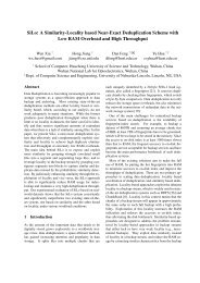
Figure 4: Online profiling process
54 WebApps ’11: <strong>2nd</strong> <strong>USENIX</strong> <strong>Conference</strong> on Web Application Development <strong>USENIX</strong> Association
s =
r1
1+ λ1×r1
n
(4)
where n is the number of CPU cores of this machine
(as announced by the Cloud provider). The service time
is the response time of the instance under low workload
where the effects of request concurrency are negligible.
It indicates the capability of the instance to serve incoming
requests. We can then use this service time to derive
a first performance profile of the new instance as follows:
s
r(λ) =
1 − λ×s
(5)
n
Figure 4(b) shows the first performance profile of the
new instance derived based on the calculated service
time. One should however note that this profile built out
of a single performance value is very approximate. For
a more precise profile, one needs to measure more data
points.
Using this profile, we can now calculate a second
workload intensity which should bring the instance close
to the SLO. We select an expected response time r2, then
derive the workload intensity which should produce this
response time.
r expected
2 =0.8 × SLO (6)
λ2 =
n × (rexpected
2
r expected
2
− s)
× s
(7)
Here we set the target response time to 80% of the
SLO to avoid violating the SLO of the profiled instance
even though the initial performance profile will feature
relatively large error margins. We can then address this
workload intensity to the new instance and measure its
real performance value (λ2, r2). As shown in Figure 4(c),
the real performance of the second point is somewhat different
from the expected 80% of the SLO.
We apply linear regression between the two measured
points (λ1, r1), (λ2, r2) and get the fitted performance
profile of the new instance as shown in Figure 4(d). We
then let the load balancer calculate the weighted workload
distribution between the provisioned instance and
the new one.
By addressing the weighted workload intensities to the
two instances, we can measure the real response time of
the new instance. However, as shown in Figure 4(e), the
real performance of the new instance differs slightly from
the expected one in Figure 4(d) due to the approximation
error of its initial profile. We then correct the performance
profile of the new instance by interpolating the
third performance point(λ3, r3). We show that the above
strategy is effective to profile heterogeneous virtual machines
and provision single services in Section 5.