Stochastic formalism revisited: a self-consistent recursive approach

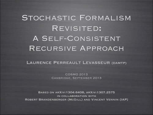
Stochastic FormalismRevisited:A Self-ConsistentRecursive ApproachLaurence Perreault Levasseur (DAMTP)COSMO 2013Cambridge, September 2013Based on arXiv:1304.6408, arXiv:1307.2575in collaboration withRobert Brandenberger (McGill) and Vincent Vennin (IAP)

Back to the basics

Back to the basicsSplit:ˆ = ' +

Back to the basicsSplit:ˆ = ' +ClassicalBackground (fixed)homogeneous)acceleration

Back to the basicsSplit:ˆ = ' +ClassicalBackground (fixed)Small quantumperturbationshomogeneous acceleration Structure)Quantum fluctuations: are created on small scales, are stretched bythe inflating space beyond the Hubble radius where they freeze out(when k/aH ⇠ 1), get squeezed and undergo classicalisation. (they laterre-enter the Hubble, and seed the fluctuations of the CMB and the LLS of the Universe)

Back to the basicsSplit:ˆ = ' +ClassicalBackground (fixed)Small quantumperturbationshomogeneous acceleration Structure)Quantum fluctuations: are created on small scales, are stretched bythe inflating space beyond the Hubble radius where they freeze out(when k/aH ⇠ 1), get squeezed and undergo classicalisation. (they laterre-enter the Hubble, and seed the fluctuations of the CMB and the LLS of the Universe)Is this split accurate/good?

Back to the basicsSplit:ˆ = ' +ClassicalBackground (fixed)Small quantumperturbationshomogeneous acceleration Structure)Quantum fluctuations: are created on small scales, are stretched bythe inflating space beyond the Hubble radius where they freeze out(when k/aH ⇠ 1), get squeezed and undergo classicalisation. (they laterre-enter the Hubble, and seed the fluctuations of the CMB and the LLS of the Universe)Is this split accurate/good?Idea: we are interested in the classical theory, beyond the Hubbleradius, since these are the range of scales that are observable in theCMB.) Write an effective classical theory for these modes,by coarse-graining, or averaging, over scales ⇠ H 1

«Problem»: Modes smaller than the coarsegrainingscale, that is quantum-fluctuatingmodes, are constantly escaping the coarsegrainedregion and sourcing the classical theory.From this perspective, they act as a noise for theclassical theory

«Problem»: Modes smaller than the coarsegrainingscale, that is quantum-fluctuatingmodes, are constantly escaping the coarsegrainedregion and sourcing the classical theory.From this perspective, they act as a noise for theclassical theoryStochastic inflation describes how to performthis averaging, and how quantum fluctuationgive rise to a classical noise term in the effectivecoarse-grained classical equation.

Why does this evenmatter?Shouldn’t the constant contribution of incoming quantum modes into thecoarse grained theory be negligible anyway?

Why does this evenmatter?Shouldn’t the constant contribution of incoming quantum modes into thecoarse grained theory be negligible anyway?- Matters a lot, e.g. when the classical trajectory in field space isconstrained to small fields values, quantum dispersion may dominates

Why does this evenmatter?Shouldn’t the constant contribution of incoming quantum modes into thecoarse grained theory be negligible anyway?- Matters a lot, e.g. when the classical trajectory in field space isconstrained to small fields values, quantum dispersion may dominates- Also, in eternal inflation, quantum corrections must dominate overthe classical trajectory

Why does this evenmatter?Shouldn’t the constant contribution of incoming quantum modes into thecoarse grained theory be negligible anyway?- Matters a lot, e.g. when the classical trajectory in field space isconstrained to small fields values, quantum dispersion may dominates- Also, in eternal inflation, quantum corrections must dominate overthe classical trajectoryIn general,allows to constantly «renormalise» the background trajectory,i.e. re-sums the incoming quantum modes in the background.so e.g. H(t) assumes it physical values at all t) Powerful non-perturbative method

How does it work?(Heuristically)Consider a set of 2 quantum fieldsnˆ, ˆ o(generalisation to largernumbers easy)Split each one into long and short wavelengths at a coarse grainingscale using a window function= ' + > , = + > ,> , > correspond to k>H(t)a(t) ,' , correspond to H(t)a(t) >k>0 ,

How does it work?(Heuristically)Consider a set of 2 quantum fieldsnˆ, ˆ o(generalisation to largernumbers easy)Split each one into long and short wavelengths at a coarse grainingscale using a window function= ' + > , = + > ,> , > correspond to k>H(t)a(t) ,' , correspond to H(t)a(t) >k>0 ,Goal: Integrate out the high k degrees of freedom.- In the same spirit as Wilsonian renormalisation, we want to get afor the system fields once the bath has been integrated out.-> Similar to quantum Brownian motion!V eff

Stochastic equations of motion:⇤' + m 2 ' + V pert ,' =3H⇠⇤ + m 2 + V pert , =3H⇠

Stochastic equations of motion:⇤' + m 2 ' + V pert ,' =3H⇠⇤ + m 2 + V pert , =3H⇠These form a system of classical Langevin equations, sourced by randomgaussian noise terms (which are completely determined by their 2-pt functions).They describe a stochastic process.

Stochastic equations of motion:⇤' + m 2 ' + V pert ,' =3H⇠⇤ + m 2 + V pert , =3H⇠These form a system of classical Langevin equations, sourced by randomgaussian noise terms (which are completely determined by their 2-pt functions).They describe a stochastic process.BUT: To find the 2-pt functions, we still need the linearised mode functions:

A Recursive Method?We now have two coupled systems of 2 equations each:the classical stochastic system and the quantum systemIn order to solve it consistently, we must solve both to the sameorder of accuracy in the slow-roll parameters and in ~) We use a recursive approach!

Outline of theRecursive Approach

Outline of theRecursive Approach1. Solve for the quantum fields >, > mode functions to zerothorder in slow-roll, that is, as if they were free, massless fields in dSspace. Get the zeroth order noise:h⇠ ,1 (x,t), ⇠ ,1 (x,t)i = H3 sin(✏aHr)4⇡ 2 ✏aHr(t t 0 )

Outline of theRecursive Approach1. Solve for the quantum fields >, > mode functions to zerothorder in slow-roll, that is, as if they were free, massless fields in dSspace. Get the zeroth order noise:h⇠ ,1 (x,t), ⇠ ,1 (x,t)i = H3 sin(✏aHr)4⇡ 2 ✏aHr',3H 2 d'dN = V , + 3H32⇡ ⇠ (N) ,3H 2 d dN = V , + 3H32⇡ ⇠(N)(t t 0 )2. Use this noise to find the classical fields to zeroth order inslow-roll and their corresponding PDFs. i.e. we need to solve:where we changed the time variable to the e-fold number: N ⌘ ln(a/a i )

Recursive Approachcontinued...3. Go back to the linearised mode functions for the quantum fieldsand replace all occurrences of the coarse-grained fields by theiraverage values, variances, and higher momenta:', ! h'i, h i,' 2 ,2! h' 2 i, h 2 i,' p q ! h' p q i ,solve the corrected linearised equations for >, > , this timeexpanding to next-to-leading order in slow-roll.i.e. solve for the full linearised mode functions

Recursive Approachcontinued...3. Go back to the linearised mode functions for the quantum fieldsand replace all occurrences of the coarse-grained fields by theiraverage values, variances, and higher momenta:', ! h'i, h i,' 2 ,2! h' 2 i, h 2 i,' p q ! h' p q i ,solve the corrected linearised equations for >, > , this timeexpanding to next-to-leading order in slow-roll.i.e. solve for the full linearised mode functions4. Go back to the coarse-grained ', system, and reevaluate thePDF with the corrected linearised noise. Keep up to Oin slow-roll. Can find the spectrum, including the tilt, in aconsistent manner.✓qh⇠ ,1,2 ⇠ ,1,2 i ◆etc... until the process converges

Hybrid Inflation Two scalar fields inflation, the inflaton ! and the waterfall field " Inflation takes place when ! is slowly rolling for ! > ! c The energy density is dominated by the mass of " For ! < ! c , the " → −" symmetry is broken and " develop a tachyonicinstability, which trigger its rapid rolling toward a true ground state

Dynamics and Steps 1-2- Potential:V ( , )= 1 2 m2 2 + 4(2v 2 ) 2 + g222 2

Dynamics and Steps 1-2- Potential:V ( , )= 1 2 m2 2 + 4(2v 2 ) 2 + g222 2Recursive Solution:- Step 1: Free, massless dS noise:h⇠ ,1 (x,t), ⇠ ,1 (x,t)i = H3 sin(✏aHr)4⇡ 2 ✏aHr(t t 0 )

Dynamics and Steps 1-2- Potential:V ( , )= 1 2 m2 2 + 4(2v 2 ) 2 + g222 2Recursive Solution:- Step 1: Free, massless dS noise:h⇠ ,1 (x,t), ⇠ ,1 (x,t)i = H3 sin(✏aHr)4⇡ 2 ✏aHr(t t 0 )- Step 2: Zeroth order stochastic equations:3H 2 d'dN =m2 '✓1+ g2 2m 2 ◆3H 2 d dN = v2 ✓ '2 2c2c+◆2v 2+3H⇠ (N) ,+3H⇠(N)

- Step 2 (continued): Zeroth order stochastic solutions: Martin & Vennin 2011' =exp⌦ 2↵ 12 v 8=384⇡ 2 m 2 Mpl4"4 m2 M 2 plv 4 (N N in )✓ m 2 e x#"v 2 x' in +2◆ v 2m 2 ✓ v2m 2 , v 2m 2 x ◆r3 Mplv 2Z NN inexp,4 m2 M 2 plv 4n!⇠ (n) dn#,Zeroth order dispersions:⌘qh 2 i h i 2 =c' =v 4v 48 p 6⇡mM 2 pl8 p 6⇡mMpl2✓' 2⇡✓ m 2 e xv 2 x◆ v 22m 2 12◆ 3/4 ⇣ v⌘ 1/2 v 33m 8Mpl2..✓ v2m 2 , v 2m 2 x ◆,

Step 3Linearised quantum perturbations on a stochastically shifted background:- Replace coarse-grained quantities with their stochastic mean:Fh' (0) ,(0) i !DFh' (0) ,(0) iE .- We work in the spatially flat gauge;- The EoM & solution for the canonically normalised field,(1):v k !v 00k +"#k 2 2 m 2 /H 2 g 2 2 /H 2 +9" 1⌧ 2 v k =0(e i(⌫+ 1 2 ) ⇡ 2 2⌫ p 1⌫+1/2( ⌧)⇡(⌫)k0 < ⌫ apple 3/2⌫e i ⇡ 2 ( ⌧) 1/2 ln( k⌧) ⌫ =0k= a 1 v k⌫ 2 =9/4 (m 2 + g 2 )/H 2 +9" 1

Step 3 (continued...)Similarly, for(1)k= a 1 u ku 00 k + ⇥ k 2 m 2 u (⌧) ⇤ u k =0, m 2 u(⌧) ⌘ 2 m2 /H 2⌧ 2= 1⌧ 2 "2 + 15" 1 32H 212M 2 plv 2 ' (0)2' 2 c1!#Solution in terms of Airy functions, but not very enlightening towrite down...

Step 4: ResultsUnder the quasi-static approximation, i.e. the relaxation time for the !distribution is very small, and it swiftly acquires its “stationary” localdispersion.2 / 2 massless 'h⇠2 i/h⇠ 2 i massless = | (1) | 2 /| (1) | 2 massless) 2 '(1) 2H 4 /(4⇡ 2 )2massless

For the inflaton:- Noise amplitudeh⇠ (N) ⇠ (N 0 )i = H44⇡ 2 (N N 0 )"1+ 2 3m 2 + g 2H 2 (ln 2✏ + 2)#,- Classical perturbationsh( ' (1) ) 2 i⇡ 3H4 ' 2 ✓08⇡ 2 ˜m 2 1' 2 0(' 0 ) 2 in◆✓1+ 2 3◆AH 2) ' (1)k2⇡✓ kaH◆ 2˜m 23H 2 49˜m 4H4 (ln 2✏+ 2)with:A =˜m 2 (ln 2✏ + 2) ˜m 2 =(m 2 + g 2 2 )

Setup:Slow-Roll InflationThe quasi-exponential growth of a(t) is driven by the slow rollof a scalar field ˆ down the slope of a flat potential.¨' +3H ˙' + V ,' =0apple ˙'22 + VH 2 = 13Mpl2Assume:ˆ ⇡ '¨' ⌧ 3H ˙'⇢ ⇡ V ⇠ cst)H ⇡ cst}a(t) ⇠ e Htquasi-de Sitter) Physical lengths grow quasi-exponentially(we allow Ḣ 6= 0but do not perturb the metric for now)