Chapter 4 Applications of the definite integral to rates, velocities and ...
Chapter 4 Applications of the definite integral to rates, velocities and ...
Chapter 4 Applications of the definite integral to rates, velocities and ...

Create successful ePaper yourself
Turn your PDF publications into a flip-book with our unique Google optimized e-Paper software.
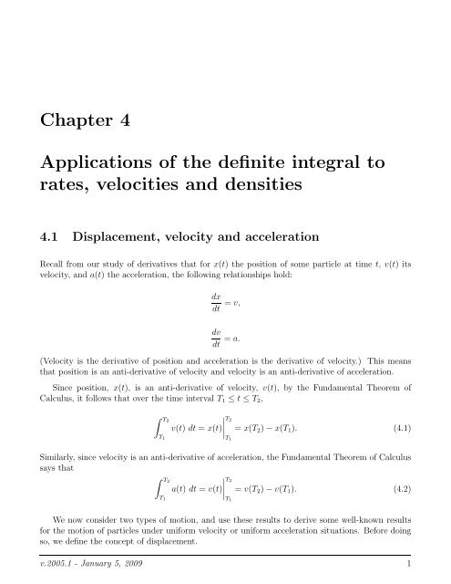
<strong>Chapter</strong> 4<strong>Applications</strong> <strong>of</strong> <strong>the</strong> <strong>definite</strong> <strong>integral</strong> <strong>to</strong><strong>rates</strong>, <strong>velocities</strong> <strong>and</strong> densities4.1 Displacement, velocity <strong>and</strong> accelerationRecall from our study <strong>of</strong> derivatives that for x(t) <strong>the</strong> position <strong>of</strong> some particle at time t, v(t) itsvelocity, <strong>and</strong> a(t) <strong>the</strong> acceleration, <strong>the</strong> following relationships hold:dxdt = v,dvdt = a.(Velocity is <strong>the</strong> derivative <strong>of</strong> position <strong>and</strong> acceleration is <strong>the</strong> derivative <strong>of</strong> velocity.) This meansthat position is an anti-derivative <strong>of</strong> velocity <strong>and</strong> velocity is an anti-derivative <strong>of</strong> acceleration.Since position, x(t), is an anti-derivative <strong>of</strong> velocity, v(t), by <strong>the</strong> Fundamental Theorem <strong>of</strong>Calculus, it follows that over <strong>the</strong> time interval T 1 ≤ t ≤ T 2 ,∫ T2T 1T 2v(t) dt = x(t)∣ = x(T 2 ) − x(T 1 ). (4.1)T 1Similarly, since velocity is an anti-derivative <strong>of</strong> acceleration, <strong>the</strong> Fundamental Theorem <strong>of</strong> Calculussays that∫ T2T 2a(t) dt = v(t)∣ = v(T 2 ) − v(T 1 ). (4.2)T 1T 1We now consider two types <strong>of</strong> motion, <strong>and</strong> use <strong>the</strong>se results <strong>to</strong> derive some well-known resultsfor <strong>the</strong> motion <strong>of</strong> particles under uniform velocity or uniform acceleration situations. Before doingso, we define <strong>the</strong> concept <strong>of</strong> displacement.v.2005.1 - January 5, 2009 1
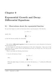
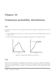
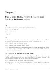
Math 103 Notes <strong>Chapter</strong> 4DisplacementThe displacement, x(T 2 )−x(T 1 ), <strong>of</strong> a particle, over <strong>the</strong> time interval T 1 ≤ t ≤ T 2 is <strong>the</strong> net differencebetween its final <strong>and</strong> initial positions. For example, if you drive from home <strong>to</strong> work in <strong>the</strong> morning,<strong>and</strong> drive back at night, <strong>the</strong>n your displacement over that day is zero. (You may have driven a longdistance in getting <strong>the</strong>re <strong>and</strong> back.)Suppose we label <strong>the</strong> initial time zero (T 1 = 0) <strong>and</strong> <strong>the</strong> final time T (i.e. T 2 = T) <strong>the</strong>n <strong>the</strong><strong>definite</strong> <strong>integral</strong> <strong>of</strong> <strong>the</strong> velocity,∫ T0v(t) dt = x(T) − x(0),is <strong>the</strong> displacement over <strong>the</strong> time interval 0 ≤ t ≤ T.We can similarly consider <strong>the</strong> net change prescribed by equation 4.2 over this time interval:∫ TTa(t) dt = v(t)∣ = v(T) − v(0)0is <strong>the</strong> net change in velocity between time 0 <strong>and</strong> time T, (though this quantity does not have specialterminology).0Geometric interpretationsSuppose we are given a graph <strong>of</strong> <strong>the</strong> velocity v(t), as shown on <strong>the</strong> left <strong>of</strong> Figure 4.1. Then by<strong>the</strong> definition <strong>of</strong> <strong>the</strong> <strong>definite</strong> <strong>integral</strong>, we can interpret ∫ T 2T 1v(t) dt as <strong>the</strong> “area” associated with<strong>the</strong> curve (counting positive <strong>and</strong> negative contributions) between <strong>the</strong> endpoints T 1 <strong>and</strong> T 2 . Thenaccording <strong>to</strong> <strong>the</strong> above observations, this area represents <strong>the</strong> displacement <strong>of</strong> <strong>the</strong> particle between<strong>the</strong> two times T 1 <strong>and</strong> T 2 .vThis arearepresentsdisplacementaThis arearepresents netvelocity changeT 1T2tT 1T2tFigure 4.1: The <strong>to</strong>tal area under <strong>the</strong> velocity graph represents net displacement, <strong>and</strong> <strong>the</strong> <strong>to</strong>tal areaunder <strong>the</strong> graph <strong>of</strong> acceleration represents <strong>the</strong> net change in velocity over <strong>the</strong> interval T 1 ≤ t ≤ T 2 .Similarly, by previous remarks, <strong>the</strong> area under <strong>the</strong> curve a(t) is a geometric quantity thatrepresents <strong>the</strong> net change in <strong>the</strong> velocity, as shown on <strong>the</strong> right <strong>of</strong> Figure 4.1.v.2005.1 - January 5, 2009 2
Math 103 Notes <strong>Chapter</strong> 4Displacement for uniform motionWe first examine <strong>the</strong> simplest case that <strong>the</strong> velocity is constant, i.e. v(t) = v = constant. Thenclearly, <strong>the</strong> acceleration is zero since a = dv/dt = 0 when v is constant. Thus, by direct antidifferentiation,∫ TTv dt = vt∣ = v(T − 0) = vT.0However, applying result (4.1) over <strong>the</strong> time interval 0 ≤ t ≤ T also leads <strong>to</strong>∫ T00v dt = x(T) − x(0).Therefore, it must be true that <strong>the</strong> two expressions obtained above must be equal, i.e.x(T) − x(0) = vT.Thus, here, <strong>the</strong> displacement is proportional <strong>to</strong> <strong>the</strong> velocity <strong>and</strong> <strong>to</strong> <strong>the</strong> time elapsed, <strong>and</strong> <strong>the</strong> finalposition isx(T) = x(0) + vT.This is true for all time T, so we can rewrite <strong>the</strong> results in terms <strong>of</strong> <strong>the</strong> more familiar (lower case)notation for time, t, i.e.x(t) = x(0) + vt.Uniformly accelerated motionIn this case <strong>the</strong> acceleration is constant. Thus, by direct antidifferentiation,∫ TTa dt = at∣ = a(T − 0) = aT,However, using result (4.2) for 0 ≤ t ≤ T leads <strong>to</strong>0∫ T00a dt = v(T) − v(0).Since <strong>the</strong>se two, results must match, v(T) − v(0) = aT so thatv(T) = v(0) + aT.Let us refer <strong>to</strong> <strong>the</strong> initial velocity V (0) as v 0 . The above connection between velocity <strong>and</strong> accelerationholds for any final time T, i.e., it is true for all t that:v(t) = v 0 + at.This just means that velocity at time t is <strong>the</strong> initial velocity incremented by an increase (over <strong>the</strong>given time interval) due <strong>to</strong> <strong>the</strong> acceleration. From this we can find <strong>the</strong> displacement <strong>and</strong> position<strong>of</strong> <strong>the</strong> particle as follows: Let us call <strong>the</strong> initial position x(0) = x 0 . Then∫ T0v(t) dt = x(T) − x 0 .v.2005.1 - January 5, 2009 3
Math 103 Notes <strong>Chapter</strong> 4ButI =∫ T0v(t) dt =∫ T0(v 0 + at) dt =So, setting <strong>the</strong>se two results equal means that( ) ∣ ∣∣∣v 0 t + a t2 T20x(T) − x 0 = v 0 T + a T 22 .=(v 0 T + a T 22But this is true for all final times, T, i.e. this holds for any time t so that).x(t) = x 0 + v 0 t + a t2 2 .This expression represents <strong>the</strong> position <strong>of</strong> a particle at time t given that it experienced a constantacceleration, a, after starting with initial velocity v 0 , from initial position x 0 at time t = 0.Non-constant acceleration <strong>and</strong> terminal velocityThe velocity <strong>of</strong> a sky-diver is described by a differential equationdvdt = g − kvi.e., a ma<strong>the</strong>matical statement that relates changes in velocity <strong>to</strong> acceleration due <strong>to</strong> gravity, g,<strong>and</strong> drag forces due <strong>to</strong> friction with <strong>the</strong> atmosphere. A good approximation for such drag forcesis <strong>the</strong> term kv, proportional <strong>to</strong> <strong>the</strong> velocity, with k, a positive constant, representing a frictionalcoefficient. We will assume that initially <strong>the</strong> velocity is zero, i.e. v(0) = 0. In this example we showhow <strong>to</strong> determine <strong>the</strong> velocity at any time t. In this calculation, we will use <strong>the</strong> following resultfrom first term calculus material:The differential equation <strong>and</strong> initial conditiondydt = −ky, y(0) = y 0 (4.3)has a solutiony(t) = y 0 e −kt (4.4)The equation dv/dt = g − kv implies thata(t) = g − kv(t)where a(t) is <strong>the</strong> acceleration at time t. Taking a derivative <strong>of</strong> both sides <strong>of</strong> this equation leads <strong>to</strong>dadt = −kdv dt ,which means thatdadt = −ka.v.2005.1 - January 5, 2009 4
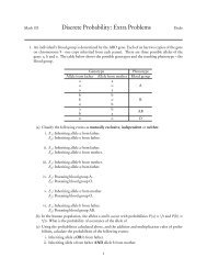
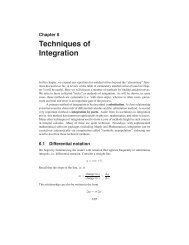
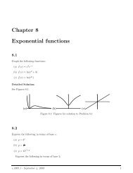
Math 103 Notes <strong>Chapter</strong> 4We observe that this equation is precisely like equation (4.3) (with a replacing y), which implies(according <strong>to</strong> 4.3) that a(t) is given bya(t) = C e −kt = a 0 e −kt .Initially, at time t = 0, <strong>the</strong> acceleration is a(0) = g (since a(t) = g −kv(t), <strong>and</strong> we have assumedthat v(0) = 0). Thena(t) = g e −kt .40302010010 20 30tFigure 4.2: Terminal velocity (m/s) for acceleration due <strong>to</strong> gravity g=9.8 m/s 2 , <strong>and</strong> k = 0.2. Thevelocity reaches a near constant 49 m/s after about 20 s.Then∫ T0a(t) dt =∫ T0g e −kt dt = g∫ T0e −kt dt = g[ ] ∣ e−kt ∣∣∣T−k0= g (e−kT − 1)−k= g k(1 − e−kT ) .As before, based on equation (4.2) <strong>the</strong> same <strong>integral</strong> <strong>of</strong> acceleration over 0 ≤ t ≤ T must equalv(T)−v(0). But v(0) = 0 by assumption, <strong>and</strong> <strong>the</strong> result is true for any final time T, so, in particular,setting T = t, <strong>and</strong> combining both results leads <strong>to</strong> an expression for <strong>the</strong> velocity at any time:v(t) = g ( ) 1 − e−kt.kWe can also determine how <strong>the</strong> velocity behaves in <strong>the</strong> long term: observe that for t → ∞, <strong>the</strong>exponential term e −kt → 0, so thatv(t) → g k (1 − very small quantity) ≈ g kThus, when drag forces are in effect, <strong>the</strong> falling object does not continue <strong>to</strong> accelerate in<strong>definite</strong>ly:it eventually attains a terminal velocity. We have seen that this limiting velocity is v = g/k. Theobject continues <strong>to</strong> fall at this (approximately constant) speed as shown in Figure 4.2.v.2005.1 - January 5, 2009 5
Math 103 Notes <strong>Chapter</strong> 44.2 From density <strong>to</strong> <strong>to</strong>tal numberThe concept <strong>of</strong> density is used widely in many applications in science. In this section, we giveseveral examples <strong>of</strong> <strong>the</strong> connection between density <strong>and</strong> <strong>to</strong>tal amount. As discussed below, thatconnection is closely related <strong>to</strong> <strong>the</strong> idea <strong>of</strong> integration.4.2.1 Density <strong>of</strong> cars along a highwayA measure <strong>of</strong> highway congestion might be <strong>the</strong> density <strong>of</strong> cars along a stretch <strong>of</strong> road. By densitywe here mean number <strong>of</strong> cars per unit distance. Suppose we want <strong>to</strong> make a connection between<strong>the</strong> <strong>to</strong>tal number <strong>of</strong> vehicles on a particular segment <strong>of</strong> <strong>the</strong> highway <strong>and</strong> <strong>the</strong>ir density along thatsegment. If <strong>the</strong> cars are spaced equal distances apart, this would be easy: Total number = densityper unit distance times <strong>the</strong> <strong>to</strong>tal length <strong>of</strong> <strong>the</strong> segment <strong>of</strong> road. However, if <strong>the</strong> cars are distributednon-uniformly, we need a better approach. Suppose we let x denote position along <strong>the</strong> highway,with x = 0 at <strong>the</strong> beginning <strong>of</strong> <strong>the</strong> segment <strong>of</strong> interest. Suppose C(x) is <strong>the</strong> density <strong>of</strong> cars atposition x.We might subdivide <strong>the</strong> road up in<strong>to</strong> small sections each <strong>of</strong> length ∆x, <strong>and</strong> approximate <strong>the</strong>number <strong>of</strong> cars on each <strong>of</strong> <strong>the</strong>se small segments by C(x)∆x. If those segments are small enough,this should be a relatively good approximation. The Total number <strong>of</strong> cars all along <strong>the</strong> road would<strong>the</strong>n be∑C(x)∆xwhere <strong>the</strong> sum extends from x = 0 <strong>to</strong> <strong>the</strong> end <strong>of</strong> <strong>the</strong> highway, at some place x = L. From this idea,we find that <strong>the</strong>re is a connection between <strong>the</strong> <strong>to</strong>tal number <strong>and</strong> <strong>the</strong> <strong>integral</strong> <strong>of</strong> <strong>the</strong> density, i.e.,that∫ L0C(x) dx = Total number <strong>of</strong> cars.ExampleAt rush hour, <strong>the</strong> density <strong>of</strong> cars along a highway is given byC(x) = 100x(1 − x 10 ) 0 ≤ x ≤ Lwhere x is distance in kilometers(a) What is <strong>the</strong> largest value <strong>of</strong> L for which this density makes sense?(b) Where along <strong>the</strong> highway is <strong>the</strong> congestion greatest? What is <strong>the</strong> car density at that location?(c) What is <strong>the</strong> <strong>to</strong>tal number <strong>of</strong> cars along <strong>the</strong> road?Solution(a) Density has <strong>to</strong> be a positive quantity. Therefore L = 10 is <strong>the</strong> largest allowable value <strong>of</strong> x. Thisformula would break down outside <strong>of</strong> <strong>the</strong> range 0 ≤ x ≤ 10.v.2005.1 - January 5, 2009 6
Math 103 Notes <strong>Chapter</strong> 4(b) Greatest highest congestion is equivalent <strong>to</strong> greatest density. To find this, we look fora maximum in <strong>the</strong> function C(x), e.g. by setting its derivative <strong>to</strong> zero. We find that C ′ (x) =100 − 20x = 0 leads <strong>to</strong> x = 5, so <strong>the</strong> greatest congestion is in <strong>the</strong> middle <strong>of</strong> <strong>the</strong> road, at x = 5 km.At this location, we have C(5) = 250 cars per kilometer.(c) The <strong>to</strong>tal number <strong>of</strong> cars on <strong>the</strong> road (assuming that we take L = 10) isI =∫ L0C(x) dx =∫ LWe calculate <strong>the</strong> above <strong>integral</strong>:( x2I = 1002 − 1 100100x(1 − x ∫ 1010 ) dx = (100x − 10x 2 ) dx.) ∣x 3 ∣∣∣10 ( 1= 10 4302 − 1 )= 1043 6Thus, <strong>the</strong>re are 1,666 cars over <strong>the</strong> ten kilometers highway at rush hour.0= 1, 6664.3 From <strong>rates</strong> <strong>of</strong> change <strong>to</strong> <strong>to</strong>tal changeIn this section, we examine several examples in which <strong>the</strong> rate <strong>of</strong> change <strong>of</strong> some process is specified.We use this information <strong>to</strong> obtain <strong>the</strong> net (<strong>to</strong>tal) change that occurs over some time period.Changing temperatureWe must carefully distinguish between information about <strong>the</strong> time dependence <strong>of</strong> some function,from information about <strong>the</strong> rate <strong>of</strong> change <strong>of</strong> some function. Here is an example <strong>of</strong> <strong>the</strong>se twodifferent cases, <strong>and</strong> how we would h<strong>and</strong>le <strong>the</strong>m(a) The temperature <strong>of</strong> a cup <strong>of</strong> juice is observed <strong>to</strong> beT(t) = 25(1 − e −0.1t )in degrees Celsius where t is time in minutes. Find <strong>the</strong> change in <strong>the</strong> temperature <strong>of</strong> <strong>the</strong> juicebetween t = 1 <strong>and</strong> t = 5.Solution(a) In this case, we are given <strong>the</strong> temperature as a function <strong>of</strong> time. To determine what netchange occurred between times t = 1 <strong>and</strong> t = 5, we would find <strong>the</strong> temperatures at each timepoint <strong>and</strong> subtract: That is, <strong>the</strong> change in temperature between times t = 1 <strong>and</strong> t = 5 is simplyT(5) − T(1) = 25(1 − e −0.5 ) − 25(1 − e −0.1 ) = 25(0.94 − 0.606) = 7.47.(b) The rate <strong>of</strong> change <strong>of</strong> temperature <strong>of</strong> a cup <strong>of</strong> c<strong>of</strong>fee is observed <strong>to</strong> bef(t) = 8e −0.2tdegree Celsius per minute where t is time in minutes. What is <strong>the</strong> <strong>to</strong>tal change in <strong>the</strong> temperaturebetween t = 1 <strong>and</strong> t = 5 minutes ?v.2005.1 - January 5, 2009 7
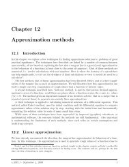
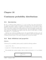
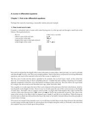
Math 103 Notes <strong>Chapter</strong> 4Solution(b) Here, we do not know <strong>the</strong> temperature at any time, but we are given information about <strong>the</strong>rate <strong>of</strong> change. (Carefully note <strong>the</strong> subtle difference in <strong>the</strong> wording.) The <strong>to</strong>tal change is foundby integrating <strong>the</strong> rate <strong>of</strong> change, f(t), from t = 1 <strong>to</strong> t = 5, i.e. by calculatingI =∫ 51f(t) dt =∫ 51∣ ∣∣∣58e −0.2t dt = −40e −0.2t = −40e −1 + 40e −0.2I = 40(e −0.2 − e −1 ) = 40(0.8187 − 0.3678) = 18.14.3.1 Tree growth <strong>rates</strong>Growthrate210 1 2 34 yearFigure 4.3: Growth <strong>rates</strong> <strong>of</strong> two trees.The rate <strong>of</strong> growth in height for two species <strong>of</strong> trees (in feet per year) is shown in Figure 4.3. If<strong>the</strong> trees start at <strong>the</strong> same height, which tree is taller after 1 year? After 4 years?SolutionWe recognize that <strong>the</strong> net change in height <strong>of</strong> each tree is <strong>of</strong> <strong>the</strong> formH i (T) − H i (0) =∫ T0g i (t)dt,where g i (t) is <strong>the</strong> growth rate as a function <strong>of</strong> time (shown for each tree in Figure 4.3) <strong>and</strong> H i (t)is <strong>the</strong> height <strong>of</strong> tree “i” at time t. But, by <strong>the</strong> Fundamental Theorem <strong>of</strong> Calculus, this <strong>definite</strong><strong>integral</strong> corresponds <strong>to</strong> <strong>the</strong> area under <strong>the</strong> curve g i (t) from t = 0 <strong>to</strong> t = T. Thus we must interpret<strong>the</strong> net change in height for each tree as <strong>the</strong> area under its growth curve. We see from Figure 4.3that at 1 year, <strong>the</strong> area under <strong>the</strong> curve for tree 1 is greater, so it has grown more. After 4 years<strong>the</strong> area under <strong>the</strong> second curve is greatest so tree 2 has grown most by that time.v.2005.1 - January 5, 2009 8
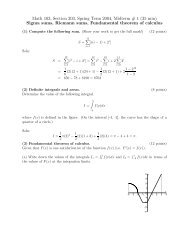
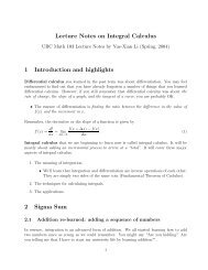
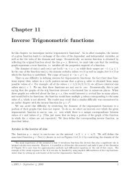
Math 103 Notes <strong>Chapter</strong> 44.3.2 Radius <strong>of</strong> a tree trunk2.521.510.50 2 4 6 8 10 12 14tFigure 4.4: Rate <strong>of</strong> change <strong>of</strong> radius, f(t) for a growing tree.The trunk <strong>of</strong> a tree, assumed <strong>to</strong> have <strong>the</strong> shape <strong>of</strong> a cylinder, grows incrementally, so that itscross-section consists <strong>of</strong> “rings”. In years <strong>of</strong> plentiful rain <strong>and</strong> adequate nutrients, <strong>the</strong> tree growsfaster than in years <strong>of</strong> drought or poor soil conditions. Suppose <strong>the</strong> rainfall pattern has been cyclic,so that, over a period <strong>of</strong> 10 years, <strong>the</strong> growth rate <strong>of</strong> <strong>the</strong> radius <strong>of</strong> <strong>the</strong> tree trunk (in cm/year) isgiven by <strong>the</strong> functionf(t) = 1.5 + sin(πt/5),shown in Figure 4.4. Let <strong>the</strong> height <strong>of</strong> <strong>the</strong> tree (<strong>and</strong> its trunk) be approximately constant over thisten year period, <strong>and</strong> assume that <strong>the</strong> density <strong>of</strong> <strong>the</strong> trunk is approximately 1 gm/cm 3 .(a) If <strong>the</strong> radius was initially r 0 at time t = 0, what will <strong>the</strong> radius <strong>of</strong> <strong>the</strong> trunk be at time tlater?(b) What will be <strong>the</strong> ratio <strong>of</strong> its final <strong>and</strong> initial mass?Solution(a) The rate <strong>of</strong> change <strong>of</strong> <strong>the</strong> radius <strong>of</strong> <strong>the</strong> tree is given by <strong>the</strong> function f(t), <strong>and</strong> we are <strong>to</strong>ld thatat t = 0, R(0) = r 0 . A graph <strong>of</strong> this growth rate over <strong>the</strong> first fifteen years is shown in Figure 4.4.The net change in <strong>the</strong> radius isR(t) − R(0) =∫ t0f(s) ds =∫ t0(1.5 + sin(πs/5)) ds.v.2005.1 - January 5, 2009 9
Math 103 Notes <strong>Chapter</strong> 4Integrating <strong>the</strong> above, we getR(t) − R(0) =(1.5t − cos(πs/5) ) ∣ ∣∣∣t.π/50Thus, using <strong>the</strong> initial value, R(0) = r 0 (which is a constant), <strong>and</strong> evaluating <strong>the</strong> <strong>integral</strong>, leads <strong>to</strong>R(t) = r 0 + 1.5t − 5 cos(πt/5)π(The constant at <strong>the</strong> end <strong>of</strong> <strong>the</strong> expression stems from <strong>the</strong> fact that cos(0) = 1.) A graph <strong>of</strong> <strong>the</strong>radius <strong>of</strong> <strong>the</strong> tree over time (using r 0 = 1) is shown in Figure 4.5. This function is equivalent <strong>to</strong><strong>the</strong> area associated with <strong>the</strong> function shown in Figure 4.4. Notice that Figure 4.5 confirms that <strong>the</strong>radius keeps growing over <strong>the</strong> entire period, but that its growth rate (slope <strong>of</strong> <strong>the</strong> curve) alternatesbetween higher <strong>and</strong> lower values.+ 5 π .25201510502 4 6 8 10 12 14tFigure 4.5: Rate <strong>of</strong> change <strong>of</strong> radius, f(t) for a growing tree.After ten years we haveBut cos(2π) = 1, soR(10) = r 0 + 15 − 5 π cos(2π) + 5 π .R(10) = r 0 + 15.(b) The mass <strong>of</strong> <strong>the</strong> tree is density times volume, <strong>and</strong> since <strong>the</strong> density is taken <strong>to</strong> be 1 gm/cm 3 ,we need only obtain <strong>the</strong> initial <strong>and</strong> final volume. Taking <strong>the</strong> trunk <strong>to</strong> be cylindrical means that <strong>the</strong>volume at a given time isV (t) = πR(t) 2 h.v.2005.1 - January 5, 2009 10
Math 103 Notes <strong>Chapter</strong> 4The ratio <strong>of</strong> final <strong>and</strong> initial volumes (<strong>and</strong> hence <strong>the</strong> ratio <strong>of</strong> final <strong>and</strong> initial mass) is( ) 2V (10)V (0) = π[R(10)]2 hπr0 2h= [R(10)]2 r0 + 15= .r02 r 04.3.3 Birth <strong>rates</strong> <strong>and</strong> <strong>to</strong>tal birthsAfter World War II, <strong>the</strong> birth rate in western countries increased dramatically. Suppose that <strong>the</strong>number <strong>of</strong> babies born (in millions per year) was given bywhere t is time in years after <strong>the</strong> end <strong>of</strong> <strong>the</strong> war.b(t) = 5 + 2t, 0 ≤ t ≤ 10(a) How many babies in <strong>to</strong>tal were born during this time period (i.e in <strong>the</strong> first 10 years after<strong>the</strong> war)?(b) Find <strong>the</strong> time T 0 such that <strong>the</strong> <strong>to</strong>tal number <strong>of</strong> babies born from <strong>the</strong> end <strong>of</strong> <strong>the</strong> war up <strong>to</strong><strong>the</strong> time T 0 was precisely 14 million.Solution(a) To find <strong>the</strong> number <strong>of</strong> births, we would integrate <strong>the</strong> birth rate, b(t) over <strong>the</strong> given time period.The net change in <strong>the</strong> population due <strong>to</strong> births (neglecting deaths) isP(10) − P(0) =∫ 100b(t) dt =∫ 100(5 + 2t) dt = (5t + t 2 )| 100 = 50 + 100 = 150[million babies].(b) Denote by T <strong>the</strong> time at which <strong>the</strong> <strong>to</strong>tal number <strong>of</strong> babies born was 14 million. Then, [inunits <strong>of</strong> million]I =I =∫ T0∫ T0b(t) dt = 14(5 + 2t) dt = 5T + T 2But ⇒ 5T + T 2 = 14 ⇒ T 2 + 5T − 14 = 0 ⇒ (T − 2)(T + 7) = 0. This has two solutions, but wereject T = −7 since we are looking for time after <strong>the</strong> War. Thus we find that T = 2 years, i.e it<strong>to</strong>ok two years for 14 million babies <strong>to</strong> have been born.4.4 Production <strong>and</strong> removalThe process <strong>of</strong> integration can be used <strong>to</strong> convert <strong>rates</strong> <strong>of</strong> production <strong>and</strong> removal in<strong>to</strong> net amountspresent at a given time. The example in this section is <strong>of</strong> this type. We investigate a processin which a substance accumulates as it is being produced, but disappears through some removalprocess. We would like <strong>to</strong> determine when <strong>the</strong> quantity <strong>of</strong> material increases, <strong>and</strong> when it decreases.Here we will combine both quantitative calculations <strong>and</strong> qualitative graph-interpretation skills.v.2005.1 - January 5, 2009 11
Math 103 Notes <strong>Chapter</strong> 4Circadean rhythm in hormone levelsConsider a hormone whose level in <strong>the</strong> blood at time t will be denoted by H(t). We will assumethat <strong>the</strong> level <strong>of</strong> hormone is regulated by two separate processes: one might be <strong>the</strong> secretion rate <strong>of</strong>specialized cells that produce <strong>the</strong> hormone. (The production rate <strong>of</strong> hormone might depend on <strong>the</strong>time <strong>of</strong> day, in some cyclic pattern that repeats every 24 hours or so.) This type <strong>of</strong> cyclic patternis called circadean rhythm. A competing process might be <strong>the</strong> removal <strong>of</strong> hormone (or its activedeactivation by some enzymes secreted by o<strong>the</strong>r cells.) In this example we will assume that both<strong>the</strong> production rate, p(t), <strong>and</strong> <strong>the</strong> removal rate, r(t) <strong>of</strong> <strong>the</strong> hormone are time-dependent, periodicfunctions with somewhat different phases.hormone production/removal <strong>rates</strong>r(t)p(t)0 3 6 9 12 3 6 9 0(noon)hourFigure 4.6: The rate <strong>of</strong> hormone production p(t) <strong>and</strong> <strong>the</strong> rate <strong>of</strong> removel r(t) are shown here. Wewant <strong>to</strong> use <strong>the</strong>se graphs <strong>to</strong> deduce when <strong>the</strong> level <strong>of</strong> hormone is highest <strong>and</strong> lowest.A typical example <strong>of</strong> two such functions are shown in Figure 4.6. This figure shows <strong>the</strong> production<strong>and</strong> removal <strong>rates</strong> over a period <strong>of</strong> 24 hours, starting at midnight. Our first task will be <strong>to</strong> useproperties <strong>of</strong> <strong>the</strong> graph in Figure 4.6 <strong>to</strong> answer <strong>the</strong> following questions:1. When is <strong>the</strong> production rate, p(t), maximal?2. When is <strong>the</strong> removal rate r(t) minimal?3. At what time is <strong>the</strong> hormone level in <strong>the</strong> blood highest?4. At what time is it lowest?5. Find <strong>the</strong> maximal level <strong>of</strong> hormone in <strong>the</strong> blood over <strong>the</strong> period shown, assuming that itsbasal (lowest) level is H = 0.Solutions1. Production rate is maximal at about 9:00 am.v.2005.1 - January 5, 2009 12
Math 103 Notes <strong>Chapter</strong> 42. Removal rate is minimal at noon.3. To answer this question we note that <strong>the</strong> <strong>to</strong>tal amount <strong>of</strong> hormone produced over a timeperiod a ≤ t ≤ b isP <strong>to</strong>tal =∫ bap(t)dt.The <strong>to</strong>tal amount removed over time interval a < t < b isR <strong>to</strong>tal =∫ bar(t)dt.This means that <strong>the</strong> net change in hormone level over <strong>the</strong> given time interval (amount producedminus amount removed) isH(b) − H(a) = P <strong>to</strong>tal − R <strong>to</strong>tal =∫ ba(p(t) − r(t))dt.We interpret this <strong>integral</strong> as <strong>the</strong> area between <strong>the</strong> curves p(t) <strong>and</strong> r(t). But we must usecaution here: For any time interval over which p(t) > r(t), this <strong>integral</strong> will be positive,<strong>and</strong> <strong>the</strong> hormone level will have increased. O<strong>the</strong>rwise, if r(t) < p(t), <strong>the</strong> <strong>integral</strong> yields anegative result, so that <strong>the</strong> hormone level has decreased. This makes simple intuitive sense: Ifproduction is greater than removal, <strong>the</strong> level <strong>of</strong> <strong>the</strong> substance is accumulating, whereas in <strong>the</strong>opposite situation, <strong>the</strong> substance is decreasing. With <strong>the</strong>se remarks, we find that <strong>the</strong> hormonelevel in <strong>the</strong> blood will be greatest at 3:00 pm, when <strong>the</strong> greatest (positive) area between <strong>the</strong>two curves has been obtained.4. Similarly, <strong>the</strong> least hormone level occurs after a period in which <strong>the</strong> removal rate has beenlarger than production for <strong>the</strong> longest stretch. This occurs at 3:00 am, just as <strong>the</strong> curves crosseach o<strong>the</strong>r.5. Here we will practice integration by actually fitting some cyclic functions <strong>to</strong> <strong>the</strong> graphs shownin <strong>the</strong> Figure. Our first observation is that if <strong>the</strong> length <strong>of</strong> <strong>the</strong> cycle (also called <strong>the</strong> period)is 24 hours, <strong>the</strong>n <strong>the</strong> frequency <strong>of</strong> <strong>the</strong> oscillation is ω = (2π)/24 = π/12. We fur<strong>the</strong>r observethat <strong>the</strong> functions shown in <strong>the</strong> Figure 4.7 have <strong>the</strong> formp(t) = A(1 + sin(ωt)),r(t) = A(1 + cos(ωt)).Intersection points occur whenp(t) = r(t)A(1 + sin(ωt)) = A(1 + cos(ωt)),sin(ωt) = cos(ωt)),⇒ tan(ωt) = 1.This last equality leads <strong>to</strong> ωt = π/4, 5π/4. But <strong>the</strong>n, using <strong>the</strong> fact that ω = π/12 we findthat t = 3, 15. Thus, over <strong>the</strong> time period 3 ≤ t ≤ 15 hrs, <strong>the</strong> hormone level is increasing. Wecan now compute <strong>the</strong> net increase in hormone over this period. For simplicity, we will takev.2005.1 - January 5, 2009 13
Math 103 Notes <strong>Chapter</strong> 421.510.505 10 15 20tFigure 4.7: The functions shown above are trigonometric approximations <strong>to</strong> <strong>the</strong> <strong>rates</strong> <strong>of</strong> hormoneproduction <strong>and</strong> removal from Figure 4.6<strong>the</strong> amplitude A = 1 from here on. In general, this would just be a multiplicative constant inwhatever solution we compute We find thatH <strong>to</strong>tal =H <strong>to</strong>tal =∫ 153∫ 153H <strong>to</strong>tal = − 12π[p(t) − r(t)] dt =∫ 15(sin π 12 t − cos π 12 t )dt =((cos 15π12After some simplifications, we find thatH <strong>to</strong>tal = − 12π3[(1 + sin(ωt)) − (1 + cos(ωt))]dt(− cos π t 12π/12 − sin π t ) ∣12 ∣∣∣15π/123)15π 3π 3π+ sin ) − (cos + sin12 12 12 )(− 4√ 22)= 24Thus <strong>the</strong> amount <strong>of</strong> hormone that accumulated over <strong>the</strong> time interval 3 ≤ t ≤ 15, i.e. between3:00 am <strong>and</strong> 3:00 pm is 24 √ 2Aπ.√2π .4.5 Average value <strong>of</strong> a functionGiven a functiony = f(x)over some interval a < x < b, we will define average value <strong>of</strong> <strong>the</strong> function as follows:v.2005.1 - January 5, 2009 14
Math 103 Notes <strong>Chapter</strong> 4DefinitionThe average value <strong>of</strong> f(x) over <strong>the</strong> interval a ≤ x ≤ b is¯f = 1b − a∫ baf(x)dx.RemarkThis type <strong>of</strong> average should not be confused with <strong>the</strong> mean or average <strong>of</strong> a distribution in <strong>the</strong>context <strong>of</strong> probability, <strong>to</strong> be seen later on in this course.Example 1Find <strong>the</strong> average value <strong>of</strong> <strong>the</strong> functiony = f(x) = x 2over <strong>the</strong> interval 2 < x < 4.Solution¯f = 14 − 2∫ 42x 2 dx = 1 2x 33∣42¯f = 1 6(4 3 − 2 3) = 28 3Example 2: Day length over <strong>the</strong> yearSuppose we want <strong>to</strong> know <strong>the</strong> average length <strong>of</strong> <strong>the</strong> day during summer <strong>and</strong> spring. We will assumethat day length follows a simple periodic behaviour, with a cycle length <strong>of</strong> 1 year (365 days). Letus measure time t in days, with t = 0 at <strong>the</strong> spring equinox, i.e. <strong>the</strong> date in spring when night <strong>and</strong>day lengths are equal. (On that data, <strong>the</strong> length <strong>of</strong> <strong>the</strong> day is 12 hrs.) We will refer <strong>to</strong> <strong>the</strong> number<strong>of</strong> daylight hours on day t by <strong>the</strong> function f(t). (We will also call f(t) <strong>the</strong> length (in hours) <strong>of</strong> <strong>the</strong>day during a given part <strong>of</strong> <strong>the</strong> year.)A simple function that would describe <strong>the</strong> cyclic changes <strong>of</strong> day length over <strong>the</strong> seasons is( ) 2πtf(t) = 12 + 4 sin365The average day length over spring <strong>and</strong> summer, i.e. over <strong>the</strong> first (365/2) ≈ 182 days is:v.2005.1 - January 5, 2009 15
Math 103 Notes <strong>Chapter</strong> 416.016.00.0 summerwinter0.0 365.00.0 summerwinter0.0 365.0Figure 4.8: We show <strong>the</strong> variations in day length (cyclic curve) as well as <strong>the</strong> average day length(height <strong>of</strong> rectangle) in this figure.¯f = 1 ∫ 182182= 1182= 1182= 11820∫ 1820f(t)dt (4.5)(12 + 4 sin( πt )182 ) dt (4.6)(12t − 4 · 182 cos( πt ) ∣ ∣∣∣182π 182 ) 0(12 · 182 − 4 · 182 [cos(π) − cos(0)]π)(4.7)(4.8)= 12 + 8 π≈ 14.546 (4.9)Thus, on average, <strong>the</strong> day is 14.546 hrs long during <strong>the</strong> spring <strong>and</strong> summer.In Figure 4.8, we show <strong>the</strong> entire day length cycle over one year. It is left as an exercise for <strong>the</strong>reader <strong>to</strong> show with a similar calculation that <strong>the</strong> average value <strong>of</strong> f over <strong>the</strong> entire year is 12 hrs.(This makes intuitive sense, since overall, <strong>the</strong> short days in winter will average out with <strong>the</strong> longerdays in summer.)Figure 4.8 also shows geometrically what <strong>the</strong> average value <strong>of</strong> <strong>the</strong> function represents. Supposewe determine <strong>the</strong> area associated with <strong>the</strong> graph <strong>of</strong> f(x) over <strong>the</strong> interval <strong>of</strong> interest. (This area ispainted red (dark) in Figure 4.8, where <strong>the</strong> interval is 0 ≤ t ≤ 365, i.e. <strong>the</strong> whole year.) Now letus draw in a rectangle over <strong>the</strong> same interval (0 ≤ t ≤ 365) having <strong>the</strong> same <strong>to</strong>tal area. (See bigrectangle in Figure 4.8, <strong>and</strong> note that its area matches with <strong>the</strong> darker, red region.) The height <strong>of</strong><strong>the</strong> rectangle represents <strong>the</strong> average value <strong>of</strong> f(t) over <strong>the</strong> interval <strong>of</strong> interest.v.2005.1 - January 5, 2009 16