Chapter 4 Applications of the definite integral to rates, velocities and ...

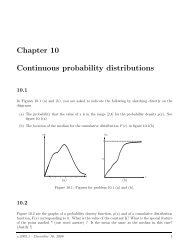
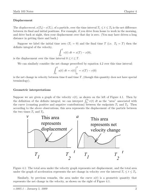
Math 103 Notes Chapter 4DisplacementThe displacement, x(T 2 )−x(T 1 ), of a particle, over the time interval T 1 ≤ t ≤ T 2 is the net differencebetween its final and initial positions. For example, if you drive from home to work in the morning,and drive back at night, then your displacement over that day is zero. (You may have driven a longdistance in getting there and back.)Suppose we label the initial time zero (T 1 = 0) and the final time T (i.e. T 2 = T) then thedefinite integral of the velocity,∫ T0v(t) dt = x(T) − x(0),is the displacement over the time interval 0 ≤ t ≤ T.We can similarly consider the net change prescribed by equation 4.2 over this time interval:∫ TTa(t) dt = v(t)∣ = v(T) − v(0)0is the net change in velocity between time 0 and time T, (though this quantity does not have specialterminology).0Geometric interpretationsSuppose we are given a graph of the velocity v(t), as shown on the left of Figure 4.1. Then bythe definition of the definite integral, we can interpret ∫ T 2T 1v(t) dt as the “area” associated withthe curve (counting positive and negative contributions) between the endpoints T 1 and T 2 . Thenaccording to the above observations, this area represents the displacement of the particle betweenthe two times T 1 and T 2 .vThis arearepresentsdisplacementaThis arearepresents netvelocity changeT 1T2tT 1T2tFigure 4.1: The total area under the velocity graph represents net displacement, and the total areaunder the graph of acceleration represents the net change in velocity over the interval T 1 ≤ t ≤ T 2 .Similarly, by previous remarks, the area under the curve a(t) is a geometric quantity thatrepresents the net change in the velocity, as shown on the right of Figure 4.1.v.2005.1 - January 5, 2009 2