- Page 1 and 2: THE UNIVERSITY OF HULLPredicting Ca
- Page 3 and 4: 3.4.2. Nonlinear Models ...........
- Page 5 and 6: 8.3. Mutual Information ...........
- Page 7 and 8: List of FiguresFig. 3.1 Typical pat
- Page 9 and 10: List of TablesTable 2.1The 11 facto
- Page 11 and 12: Table 6.14 Alternative number of cr
- Page 13 and 14: Table C12 Neural network results of
- Page 15 and 16: AbbreviationsNN(s): Neural Network(
- Page 17 and 18: Chapter 1 IntroductionThis thesis p
- Page 19 and 20: on. According to Bishop (1995), the
- Page 21 and 22: techniques is given. The standard c
- Page 23 and 24: A knowledge base that stores the in
- Page 25 and 26: This score is then compared to the
- Page 27 and 28: Cardiac signsRespiratory signsSysto
- Page 29 and 30: Given the ratings in Table 2.2, and
- Page 31 and 32: R11e3 z2Reg.No PATIENT_STATUS Physi
- Page 33 and 34: designed to their specific purposes
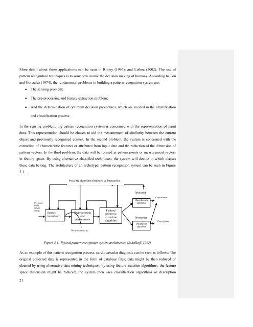
- Page 35: Chapter 3 Pattern Recognition3.1. I
- Page 39 and 40: a new patient. For example, t 5 can
- Page 41 and 42: And the strategy for pattern learni
- Page 43 and 44: Hence, whenever there is a specific
- Page 45 and 46: 3.4.2. Nonlinear ModelsDefinition:
- Page 47 and 48: vector machine are nonlinear models
- Page 49 and 50: From the confusion matrix in Table
- Page 51 and 52: the accuracy of 0.90 shows the trad
- Page 53 and 54: The comparison between neural netwo
- Page 55 and 56: Chapter 4 Supervised and Unsupervis
- Page 57 and 58: Therefore, the visualization of pat
- Page 59 and 60: A popular form of Gaussian basic fu
- Page 61 and 62: mj 1w ( x) b 0jj(4.7)where x is a
- Page 63 and 64: as an instance of the popular K-mea
- Page 65 and 66: o Update the weight as follows:w i
- Page 67 and 68: Discrete (categorical) attributes:
- Page 69 and 70: where d N (X i ,Q j ) is calculated
- Page 71 and 72: Zoo SmallThis data contains 101 cas
- Page 73 and 74: 1.20Discussions1.000.800.600.400.20
- Page 75 and 76: Chapter 5 Data Mining Methodology a
- Page 77 and 78: Raw dataDataselectingTarget DataPre
- Page 79 and 80: missing data”, the more detailed
- Page 81 and 82: Step 5 (Comparison/ Evaluation): Th
- Page 83 and 84: Missing values: The data includes 1
- Page 85 and 86: Scoring Risk Models: These are buil
- Page 87 and 88:
The missing values for the “Heart
- Page 89 and 90:
Data Filtering StageIn this step, t
- Page 91 and 92:
Supervised ClassifiersThis section
- Page 93 and 94:
5.4. SummaryData mining is a partic
- Page 95 and 96:
the significant level of 98.6% (P v
- Page 97 and 98:
Attribute nameAttributetypeMissingv
- Page 99 and 100:
Attribute nameAttributetypeMissingv
- Page 101 and 102:
6.4. Scoring Risk ModelsThe data fo
- Page 103 and 104:
are nearly the same (12). The maxim
- Page 105 and 106:
inconsistency between the linear an
- Page 107 and 108:
epochs can help to reduce the over-
- Page 109 and 110:
MSE (0.09). However, the model MLP_
- Page 111 and 112:
suitable for the CM3aD data set wit
- Page 113 and 114:
MethodA self organizing map tool is
- Page 115 and 116:
The SOM algorithm is applied to the
- Page 117 and 118:
clustering models CM3aDC and CM3bDC
- Page 119 and 120:
clustering results, resulting from
- Page 121 and 122:
and CM3bD (KMIX and SOM) suggest th
- Page 123 and 124:
equivalent rates for “High risk
- Page 125 and 126:
25 input attributes to 16 input att
- Page 127 and 128:
7.2.4. Scoring Risk ModelsThis sect
- Page 129 and 130:
increasing number of patterns impro
- Page 131 and 132:
other words, there are negligible o
- Page 133 and 134:
ACCRand = PRand(true positive true
- Page 135 and 136:
Therefore, the poor clustering perf
- Page 137 and 138:
difficulty of measuring influential
- Page 139 and 140:
“High risk” predictions in "cli
- Page 141 and 142:
chosen by the user. The methods for
- Page 143 and 144:
average information content of the
- Page 145 and 146:
MI(X , Y) H(X ) H(X | Y) pi,j( x,
- Page 147 and 148:
number of patterns in class C i ; a
- Page 149 and 150:
The results in Figure 8.3 show that
- Page 151 and 152:
and the prediction risks reflects i
- Page 153 and 154:
Adding attribute weights to the clu
- Page 155 and 156:
system. Moreover, in POSSUM and PPO
- Page 157 and 158:
in scientific and industrial applic
- Page 159 and 160:
eing located in alternative risk ba
- Page 162 and 163:
and computer scientists, to verify
- Page 164 and 165:
Baxt, W. G. (1992). Use of an Artif
- Page 166 and 167:
Cristianini, N., Shawe-Taylor, J. (
- Page 168 and 169:
Hawkins, R.G., Houston, M.C., Ferra
- Page 170 and 171:
Kohonen, T. (1981). Self-organized
- Page 172 and 173:
Manning, C.D., Raghvan, P., and Sch
- Page 174 and 175:
Ohn, M. S., Van-Nam, H., and Yoshit
- Page 176 and 177:
Simelius, K., Stenroos, M., Reinhar
- Page 178 and 179:
Wang, K. Wang, L. Wang, D. and Xu,
- Page 180 and 181:
Appendix A. Data structureA.1. Hull
- Page 182 and 183:
A.2. Dundee siteThe following table
- Page 184 and 185:
B.2. Scoring Risk ModelsTable B2 sh
- Page 186 and 187:
The results are then divided to dif
- Page 188 and 189:
Attribute NameOriginal data Transfo
- Page 190 and 191:
AttributeName175Attribute TypeMissi
- Page 192 and 193:
Filtering task: The expected outcom
- Page 194 and 195:
Data is clustered by SOM Kmeans alg
- Page 196 and 197:
197 values of “C2H”. The model
- Page 198 and 199:
PATIENT_STATUS Boolean 0 Alive/Dead
- Page 200 and 201:
Cleaning and Transformation tasks:
- Page 202 and 203:
High riskLow riskCM3a-MLPCM3a-RBFCM
- Page 204 and 205:
Table C19: Experimental results of
- Page 206 and 207:
Therefore, the Mortality has got 25
- Page 208 and 209:
Both models CM3aC and CM3bC are use
- Page 210 and 211:
R1 PATECGAMBUL_STATUR1-A SIDEANTI_A
- Page 212:
Step 5 (Building New Models): The n