Econometrics I

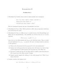
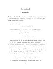
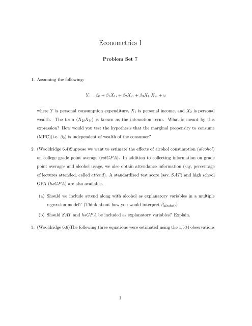
Econometrics IProblem Set 71. Assuming the following:Y i = β 0 + β 1 X 1i + β 2 X 2i + β 3 X 1i X 2i + uwhere Y is personal consumption expenditure, X 1 is personal income, and X 2 is personalwealth. The term (X 2i X 3i ) is known as the interaction term. What is meant by thisexpression? How would you test the hypothesis that the marginal propensity to consume(MPC)(i.e. β 2 ) is independent of wealth of the consumer?2. (Wooldridge 6.4)Suppose we want to estimate the effects of alcohol consumption (alcohol)on college grade point average (colGP A). In addition to collecting information on gradepoint averages and alcohol usage, we also obtain attendance information (say, percentageof lectures attended, called attend). A standardized test score (say, SAT ) and high schoolGPA (hsGP A) are also available.(a) Should we include attend along with alcohol as explanatory variables in a multipleregression model? (Think about how you would interpret β alcohol .)(b) Should SAT and hsGP A be included as explanatory variables? Explain.3. (Wooldridge 6.6)The following three equations were estimated using the 1,534 observations1

in 401K.RAW:̂prate = 80.29 + 5.44mrate + .269age − .00013totemp(.78) (.52) (.045) (.00004)R 2 = .100, ¯R 2 = .098.̂prate = 97.329 + 5.02mrate + .314age − 2.66totemp(1.95) (.51) (.044) (.28)R 2 = .144, ¯R 2 = .142.̂prate = 80.62 + 5.34mrate + .290age − .00043totemp(.78) (.52) (.045) (.00009).0000000039totemp 2(.0000000010)R 2 = .108, ¯R 2 = .106.Which of these three models do you prefer? Why?4. Using the data in SLEEP75.RAW (see also problem 3.3), we obtain the estimated equationŝleep = 3, 840.83 − .163totwork − 11.71educ − 8.70age + .128age 2 + 87.75male(235.11) (.018) (5.86) (11.21) (.134) (34.33)n = 706, R 2 = .123, ¯R 2 = .117The variable sleep is total minutes per week spent sleeping at night, totwork is total weeklyminutes spent working, educ and age are measured in years, and male is a gender dummy.(a) All other factors being equal, is there evidence that men sleep more than women ?How string is the evidence ?(b) Is there a statistically significant tradeoff between working and sleeping ? What is theestimated tradeoff ?(c) What other regression do you need to run to test the null hypothesis that, holdingother factors fixed, age has no effect on sleeping ?2

5. The following equations were estimated using the data in BWGHT.RAW:̂bwght = 4.66 − .0044cigs + .0093log(faminc) + .016parity + .027male + .055white(.22) (.0009) (.0059) (.006) (.010) (.013)n = 1, 388, R 2 = .0472.and̂bwght = 4.65 − .0052cigs + .0110log(faminc) + .017parity + .034male + .045white(.38) (.0010) (.0085) (.006) (.011) (.015)− .0030motheduc + .0032fatheduc(.0030) (.0026)n = 1, 191, R 2 = .0493.The variables are defined as in example 4.9, but we have added a dummy variable forwhether the child is male and a dummy variable indicating whether the child is classifiedas white.(a) In the first equation, interpret the coefficient on the variable cigs. In particular, whatis the effect on birth weight from smoking 10 more cigarettes per day ?(b) How much more is a white child predicted to weigh than a nonwhite child, holding theother factors in the first equation fixed ? Is the difference statistically significant?(c) Comment on the estimated effect and statistical significance of motheduc.(d) From the given information, why are you unable to compute the F statistic for jointsignificance of motheduc and fatheduc? What would you have to do to compute theF statistic?6. Using the data in GPA2.RAW, the following equation was estimated:ŝat = 1, 028.10 + 19.30hsize − 2.19hsize 2 − 45.09female − 169.81black + 62.31female · black(6.29) (3.83) (.53) (4.29) (12.71) (18.15)n = 4, 137, R 2 = .0858.3

The variable sat is the combined SAT score, hsize is size of the student’s high schoolgraduating class, in hundreds, female is a gender dummy variable, and black is a racedummy variable equal to one for blacks and zero otherwise.(a) Is there strong evidence that hsize 2 should be included in the model?From thisequation, what is the optimal high school size?(b) Holding hsize fixed, what is the estimated difference in SAT score between nonblackfemales and nonblack males? How statistically significant is this estimated difference?(c) What is the estimated difference in SAT score between nonblack males and blackmales? Test the null hypothesis that there is no difference between their scores, againstthe alternative that there is a difference.(d) What is the estimated difference in SAT score between black females and nonblackfemales? What would you need to do to test whether the difference is statisticallysignificant?4