Excel Based Finite Difference Modeling of Ground Water Flow

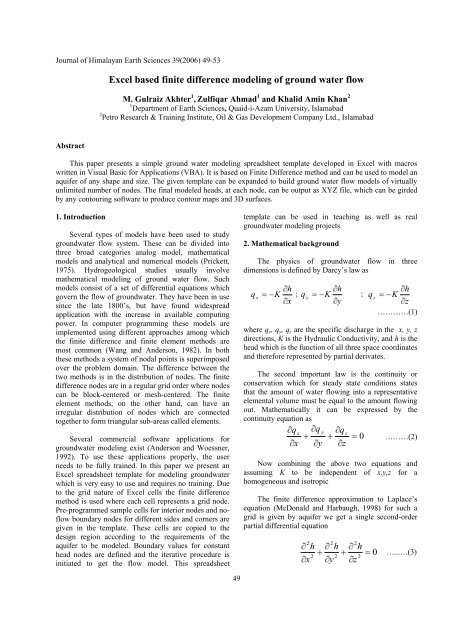
Journal of Himalayan Earth Sciences 39(2006) 49-53Excel based finite difference modeling of ground water flowM. Gulraiz Akhter 1 , Zulfiqar Ahmad 1 and Khalid Amin Khan 21 Department of Earth Sciences, Quaid-i-Azam University, Islamabad2 Petro Research & Training Institute, Oil & Gas Development Company Ltd., IslamabadAbstractThis paper presents a simple ground water modeling spreadsheet template developed in Excel with macroswritten in Visual Basic for Applications (VBA). It is based on Finite Difference method and can be used to model anaquifer of any shape and size. The given template can be expanded to build ground water flow models of virtuallyunlimited number of nodes. The final modeled heads, at each node, can be output as XYZ file, which can be girdedby any contouring software to produce contour maps and 3D surfaces.1. IntroductionSeveral types of models have been used to studygroundwater flow system. These can be divided intothree broad categories analog model, mathematicalmodels and analytical and numerical models (Prickett,1975). Hydrogeological studies usually involvemathematical modeling of ground water flow. Suchmodels consist of a set of differential equations whichgovern the flow of groundwater. They have been in usesince the late 1800’s, but have found widespreadapplication with the increase in available computingpower. In computer programming these models areimplemented using different approaches among whichthe finite difference and finite element methods aremost common (Wang and Anderson, 1982). In boththese methods a system of nodal points is superimposedover the problem domain. The difference between thetwo methods is in the distribution of nodes. The finitedifference nodes are in a regular grid order where nodescan be block-centered or mesh-centered. The finiteelement methods, on the other hand, can have anirregular distribution of nodes which are connectedtogether to form triangular sub-areas called elements.Several commercial software applications forgroundwater modeling exist (Anderson and Woessner,1992). To use these applications properly, the userneeds to be fully trained. In this paper we present anExcel spreadsheet template for modeling groundwaterwhich is very easy to use and requires no training. Dueto the grid nature of Excel cells the finite differencemethod is used where each cell represents a grid node.Pre-programmed sample cells for interior nodes and noflowboundary nodes for different sides and corners aregiven in the template. These cells are copied to thedesign region according to the requirements of theaquifer to be modeled. Boundary values for constanthead nodes are defined and the iterative procedure isinitiated to get the flow model. This spreadsheettemplate can be used in teaching as well as realgroundwater modeling projects.2. Mathematical backgroundThe physics of groundwater flow in threedimensions is defined by Darcy’s law ashhq xK ; q yK ;xyq zhKz…………(1)where q x , q y , q z are the specific discharge in the x, y, zdirections, K is the Hydraulic Conductivity, and h is thehead which is the function of all three space coordinatesand therefore represented by partial derivates.The second important law is the continuity orconservation which for steady state conditions statesthat the amount of water flowing into a representativeelemental volume must be equal to the amount flowingout. Mathematically it can be expressed by thecontinuity equation asq qx y qz0 ………(2)x y zNow combining the above two equations andassuming K to be independent of x,y,z for ahomogeneous and isotropicThe finite difference approximation to Laplace’sequation (McDonald and Harbaugh, 1998) for such agrid is given by aquifer we get a single second-orderpartial differential equation2h2x2h2y2h2z0…...…(3)49

This is Laplace’s equation which governs the flowof groundwater through an isotropic, homogeneousaquifer under steady state conditions. This equationsimply states that the sum of partial derivates of head(h) with respect to x, y, and z is zero. The solution ofLaplace’s equation requires specification of boundaryconditions such as Dirichlet conditions and Neumannconditions (Neuman, 1973). As currently we aredealing with ground water flow in two dimensionstherefore the Laplace’s equation reduces to2 2h h0 …………...(4)2 2x yFig. 1.Finite difference grid of nodes.Now consider a regularly spaced grid of nodesrepresented by i columns and j rows and horizontally andvertically spaced by distances x and y respectivelyas shown in figure 1. The head at node i ,j is h ,.2h2x2h2yhhi 1, ji,j 12hi,j( x)2h(2i,jy)2hhi 1, ji,j 1i jAdding these two terms according to Laplace’sequation and considering x y for a square gridwe haveh h h h h 0 …(5)i 1,j i 1, j i,j 1 i,j 14 i,jThe above equation is the most widely usedequation in finite difference solutions of steady-stateflow problems and forms the heart of this program. It isiteratively used in the form of a kernel or Laplacianoperator for computation of heads at each node in thegrid. Such operators are also used in satellite imageprocessing for edge detection and image smoothing (El-Sheimy et al., 2005).3. Working procedureThe complete working procedure of the presentedmodeling template is given in Figure 2. Full details forusing this template are given as a help worksheet in theExcel Modeling file. To design a new model the usersimply needs to copy and paste the required samplecells into the design region of the template (Fig. 3)according to the shape, size and type of boundaries thatdefine the aquifer. The values for constant head nodesat the boundaries are also defined.If required the iteration parameters; Maximumiterations (default 100) and Maximum change (default.001) are set using the Excel menu; Tools > Options >Calculation Tab. During each iteration the value ofheads at all nodes are calculated. The program keeps oniterating unless convergence occurs i.e. the absolutedifference in heads at each node from previous andcurrent iteration is less than the Maximum changevalue.This parameter is often critical to the modelingprocess. Too large a value will degrade the finalsolution, because convergence will not really haveoccurred. Too small a value will lead to very longexecution times and often result in no convergencebecause computational errors may cause thedifference in heads to remain larger than theMaximum change parameter. For this purpose theMaximum iteration value is also given so that theprogram does not enter into an infinite iterative loop.Thus iterations stop when conditions for either ofthese two parameters are satisfied. Now to start theiterative process the user simply needs to press F9key. The values in each cell representing a grid nodewill keep on changing unless convergence occurs anda steady state flow is attained.The modeled head values for the grid nodes can besaved as a XYZ file (X, Y are columns, rows and Z ishead) using the Visual Basic for Applications macro. Itis activated by pressing Ctrl-S keys for entering theoutput filename. The output file can be used by Surferor any other contouring software for girding andsubsequent contouring or surface generation. The finalcontour map represents the variation of head in themodeled region, where flow lines are considered to bemoving perpendicular to the contour lines from higherto lower potential.Simulation results of this spreadsheet can beutilized in different commercial software’s likePROCESSING MODFLOW (Chiang and Kinzelbach,1998) etc. to develop a complete numerical groundwater model.50

Fig. 2.Processing flow chart of the modeling template along with Surfer.Fig. 3.Excel spreadsheet template for modeling groundwater. Cells (gray to dark gray) at the top are preprogrammedfor interior nodes and various types of no-flow boundary nodes. The empty cells below formthe design region where the model is created.51

4. Practical examplesTo demonstrate the design, working and output ofthe modeling spreadsheet template two examples areshown in Figures 4 and 5. They also show the finalgraphical outputs generated by contouring software.These examples are also included in the ExcelModeling file as example worksheets. They help theuser in designing their own groundwater models in theempty spreadsheet template.5. ConclusionsIt is concluded that Excel based spreadsheetmodeling can be effectively utilized to develop theequipotential surface features of the groundwater flowregimes. Directions of groundwater flows aremonitored by assigning the vector lines at right angle tothese equipotential surfaces. Groundwater volume inactive storage can be ascertained from the completeflow-net based on Excel based spreadsheet modeling. Inaddition it can also be used, along with contouringsoftware, to generate small to large groundwater flowmodels.Fig. 4.Example of a small groundwater flow model with contour map and 3D surface from Surfer.52

Fig. 5.Example of a larger groundwater flow model with contour map from Surfer.ReferencesAnderson, M.P., Woessner, W.W., 1992. AppliedGroundwater Modeling, Academic Press, USA, 20-21.Chiang, W.H., Kinzelbach.W., 1998. (PMPATH 98).An advective transport model for ProcessingModflow and Modflow.El-Sheimy, N., Valeo, C. Habib, A., 2005. DigitalTerrain Modeling, Acquisition, Manipulation andApplications, Artech House Inc., 22-24.McDonald, M. G., Harbaugh, A, W., 1988. Amodular three-dimensional finite differenceground water flow model. Modeling Techniques,Book 6, USGS open-file report, 83-875.Neuman, S. P, 1973. Calibration of distributed parametersgroundwater flow models viewed as a multipleobjectivedecision process under uncertainty. WaterResources Research 9(4), 1006 – 1021.Prickett, T.A., 1975. Modeling Techniques forgroundwater evaluation. In advance inHydroscience. New York, Academic Press, 1-113.Wang, H.F., Anderson, M.P., 1982, Introduction togroundwater modeling – finite difference and finiteelement methods. W.H. Freeman and Company, 2-3.53