pdf reprint - Philip Sura - Florida State University

838 JOURNAL OF CLIMATE VOLUME 26Quantifying the Non-Gaussianity of Wintertime Daily Maximum and MinimumTemperatures in the SoutheastLYDIA STEFANOVACenter for Ocean–Atmospheric Prediction Studies, The Florida State University, Tallahassee, FloridaPHILIP SURACenter for Ocean–Atmospheric Prediction Studies, and Department of Earth, Ocean and Atmosphere Science,The Florida State University, Tallahassee, FloridaMELISSA GRIFFINCenter for Ocean–Atmospheric Prediction Studies, The Florida State University, Tallahassee, Florida(Manuscript received 16 March 2012, in final form 24 July 2012)ABSTRACTIn this paper the statistics of daily maximum and minimum surface air temperature at weather stations inthe southeast United States are examined as a function of the El Niño–Southern Oscillation (ENSO) andArctic Oscillation (AO) phase. A limited number of studies address how the ENSO and/or AO affect U.S.daily—as opposed to monthly or seasonal—temperature averages. The details of the effect of the ENSO orAO on the higher-order statistics for wintertime daily minimum and maximum temperatures have not beenclearly documented.Quality-controlled daily observations collected from 1960 to 2009 from 272 National Weather Service CooperativeObserving Network stations throughout Florida, Georgia, Alabama, and South and North Carolinaare used to calculate the first four statistical moments of minimum and maximum daily temperature distributions.It is found that, over the U.S. Southeast, winter minimum temperatures have higher variability thanmaximum temperatures and La Niña winters have greater variability of both minimum and maximum temperatures.With the exception of the Florida peninsula, minimum temperatures are positively skewed, whilemaximum temperatures are negatively skewed. Stations in peninsular Florida exhibit negative skewness forboth maximum and minimum temperatures. During the relatively warmer winters associated with either a LaNiña or AO1, negative skewnesses are exacerbated and positive skewnesses are reduced. To a lesser extent, theconverse is true of the El Niño and AO2. The ENSO and AO are also shown to have a statistically significanteffect on the change in kurtosis of daily maximum and minimum temperatures throughout the domain.1. IntroductionUnderstanding the statistical distribution of dailywinter temperature extremes is of practical interest tothe human endeavors in ecology, agriculture, and utilitiesplanning. This is particularly true for regions suchas the U.S. Southeast where winter hard freezes are arelatively rare and potentially catastrophic occurrence.The winter climate of the Southeast is strongly influencedCorresponding author address: Lydia Stefanova, Center forOcean–Atmospheric Prediction Studies, The Florida State University,2035 E. Paul Dirac Dr., Tallahassee, FL 32306.E-mail: lstefanova@fsu.eduby the phase of ENSO. During El Niño phase winters,the 300-hPa wind anomalies show an increased southwesterlyflow over the Gulf of Mexico (Kennedy et al.2007) as the tropical/Pacific jet splits over NorthAmerica, leading to an increased frequency of wintergulf cyclones (Eichler and Higgins 2006). In the Southeastthese contribute increased cloudiness (Angell andKorshover 1987; Angell 1990; Park and Leovy 2004) andfrequent rains (Gershunov and Barnett 1998) over theregion; as a result, the typical El Niño winter weather iswet and cool (Ropelewski and Halpert 1986, 1987;Kiladis and Diaz 1989). During the La Niña phase, thetropical/Pacific jet stream becomes a single zonal jet thatis typically shifted northward (Smith et al. 1998). TheDOI: 10.1175/JCLI-D-12-00161.1Ó 2013 American Meteorological Society

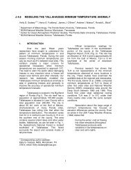
1FEBRUARY 2013 S T E F A N O V A E T A L . 839storm tracks associated with midlatitude cyclones tendto stay north of the U.S. Southeast (Eichler and Higgins2006), limiting the amount of cold air that reaches theregion; as a result, La Niña years are generally warmerand drier in the Southeast (Ropelewski and Halpert1986, 1987; Kiladis and Diaz 1989). However, variabilityin the polar jet stream position can result in extreme coldoutbreaks with either ENSO phase. In addition to theENSO phase, winter temperatures in the Southeast arestrongly influenced by the Arctic Oscillation (AO)/North Atlantic Oscillation (NAO) and to some extentPacific–North America (PNA) teleconnections (Higginset al. 2002; Hagemeyer 2006).While seasonal averages can be used as a helpfulguideline for climate application models, intraseasonalextremes are often a more important factor for practicalconsequences—a single deep freeze event in southFlorida can wreck havoc on the local agriculture(Attaway 1997). Certain agricultural crops, such ascitrus and vegetables, grown in portions of the U.S.Southeast during winter and early spring are highlysusceptible to damage from freezing temperatures. Aseries of impact freezes in the 1980s, following a seriousfreeze in 1977, left the citrus industry in Florida reeling.Approximately one-third of the state’s commercialcitrus trees were destroyed and the total monetary losswas in billions of dollars (Miller 1991). Freezing temperaturesalso have an impact on wildlife, such as theFlorida manatee. Mortality rates for manatees tend tohave a strong seasonal emphasis in winter. Manateescan die from hypothermia during unusually cold winters,as they are unable to increase heat productionby metabolism to counter losses to the environment(O’Shea et al. 1985).To understand the seasonal-scale risk of experiencingextreme cold/warm winter days, it is important to understandthe changes in distributions of daily minimum/maximum temperatures under different large-scale regimes.Do these distributions simply shift to the left orright with ENSO or AO phase change? Atmosphericvariable statistics are not strictly Gaussian (e.g., Suraet al. 2005), and daily minimum and maximum temperaturesare no exception. A shift in their expected value(warmer during La Niña, colder during El Niño) doesnot guarantee a corresponding shift for the entire distribution.The current literature is ambiguous about thetemperature extremes associated with ENSO phase.Some sources suggest that extreme cold events are morelikely with El Niño (which is associated with belownormalwinter temperatures) (e.g., Gershunov 1998;Higgins et al. 2002) or that extreme warm events aremore likely with La Niña (e.g., Wolter et al. 1999).Others (e.g., Rogers and Rohli 1991; Hansen et al. 1999;Smith and Sardeshmukh 2000) suggest that severe coldoutbreaks may be more likely with La Niña.Normal (Gaussian) distributions are fully describedby their mean and standard deviation. For non-Gaussiandistributions, higher moments need to be considered aswell. The first four moments (mean, standard deviation,skewness, and kurtosis) are generally sufficient to describemost atmospheric variable distributions. Severalstudies have documented the non-Gaussian nature ofsurface air temperatures (Toth and Szentimrey 1990;Barnston 1993; Huth et al. 2001; Ryoo et al. 2004;Shen et al. 2011). A handful ofstudies(SmithandSardeshmukh 2000; Higgins et al. 2002) have consideredthe higher (.1) statistical moments of surface temperaturesin the United States under different ENSO andAO/NAO conditions. Both studies use gridded data—from the National Centers for Environmental Prediction(NCEP) 2.58 reanalysis (Kalnay et al. 1996) inthe case of Smith and Sardeshmukh (2000) and 0.58Cooperative Observation Program (COOP) station–based gridded dataset (Janoviak et al. 1999) in the caseof Higgins et al. (2002)—and examined the response ofdaily mean surface temperatures to different largescaleclimate regime forcing.While the analysis of gridded data provides usefulinsights, gridding tends to reduce the variance of observedtemperatures (Tencer et al. 2011) and is generallyassociated with the introduction of biases in their means,especially in winter (De Gaetano and Belcher 2007) andfor maximum temperatures (De Gaetano and Belcher2007; Tencer et al. 2011). The errors introduced bygridding are highly region- and method-dependent (e.g.,Shen et al. 2005; DeGaetano and Belcher 2007; Ruppet al. 2010; Tencer et al. 2011; Berrocal et al. 2012) andare a function of station density (Legg 2011). Byits implicit smoothing, gridding filters out potentiallyvaluable spatial detail at the local and regional scale thatcan be gleaned from analysis of ungridded station data,especially near terrain features (Tencer et al. 2011; Legg2011) and coastal boundaries (De Gaetano and Belcher2007). In addition, averaging of daily minimum andmaximum surface temperatures to obtain the daily averageobscures the fact that the daily minimum andmaximum surface temperatures often have dissimilarprobability distribution function (PDF) shapes (Barnston1993; Shen et al. 2011) and disparate responses to thelarge-scale climate regimes. To illustrate this point, weconstructed PDFs of daily minimum (T min ) and maximumsurface temperatures (T max ) for two stations in theSoutheast—Charlotte, North Carolina (Fig. 1A), andFort Lauderdale, Florida (Fig. 1B), under El Niño/LaNiña and AO1/AO regimes (see Table 1 and section 2bfor the regime definitions). Such separation of T min and

840 JOURNAL OF CLIMATE VOLUME 26FIG. 1. PDF distributions for (a) Charlotte and (b) Fort Lauderdale of winter daily T max (a1, a2, b1, b2) and T min (a3, a4, b3, b4) separatedby ENSO phase (a1, a3, b1, b3) and AO phase (a2, a4, b2, b4). Solid black lines correspond to the warm regimes (either La Niña or AO1) andsolid gray lines correspond to the cold regimes (either El Niño or AO2). Dashed lines indicate the respective expected value.T max makes it possible to appreciate, for example, thatthe warming of the expected values of the daily meansassociated with El Niño relative to La Niña is largelyattributable to changes in the PDF of T max but not T minfor Charlotte, and to both T min and T max for Fort Lauderdale.The warming associated with AO1, on theother hand, stems mostly from changes in the T min distributionfor Fort Lauderdale, but is evenly contributed

1FEBRUARY 2013 S T E F A N O V A E T A L . 841TABLE 1. Summary of the ENSO and AO phase in January–February for the years 1960–2009. The number within parentheses indicatea year’s rank among the 10 years with the warmest (superscript) and coldest (subscript) January–February.Phase El Niño La Niña ENSO neutralAO1 1973, 1992, 1993 1976, 1989 (5) , 2000, 2008 1975 (3) , 1990 (1) , 2002AO2 1966 (10) , 1978 1963 (5) 1960, 1969, 1970 (6) , 1977 (2) , 1985 (8) ,1986, 2004AO neutral 1983, 1987 (1) , 1995, 1998 (6) , 2003 1962, 1967, 1971, 1974 (2) , 1999 (4) 1961, 1964, 1965, 1968 (3) , 1972, 1979 (4) ,1980, 1981 (9) , 1982, 1984, 1988 (7) ,1991 (7) , 1994, 1996, 1997 (8) , 2001,2005 (9) , 2006 (10) , 2007, 2009by T min and T max for Charlotte. In addition to theseshifts of the expected values, distinct deformations ofthe PDFs are evident as well.While it is possible to produce a catalog of all stationdistributions in different phases of these large-scale oscillations,this approach is impractical for two reasons:the need for a very large number of plots—one for eachtemperature variable at each station in every climateregime—and the lack of depiction of large-scale patternsof variability across stations. Instead, in this study wesummarize the PDFs and describe their geographicalvariability based on the distribution’s first four statisticalmoments. We examine station daily minimum (T min )and maximum (T max ) temperatures, as well as the dailyaverage (T ave ) and diurnal range (T range ) during differentENSO and AO phases. The data and methodologyused for this study are described in section 2. Results anda discussion are presented in section 3, and section 4provides a summary and concluding remarks.2. Data and methodologya. Station temperature dataWe use quality controlled digital data from the Summaryof the Day dataset (DS3200 and DS3206) suppliedby the National Climatic Data Center (NCDC). Thedaily measurements of maximum and minimum temperatureare provided by the National Weather Service’sCooperative Observation Program (COOP),which has reported these elements for over 100 years.Each dataset contains over 8000 active observing stations,though for the purpose of this study, stations wereused from the states of Alabama, Florida, Georgia,North Carolina, and South Carolina.The observing record at each station from the fiveselected states is at least from 1960 to 2009, althoughsome stations have data as far back as the early 1900s.For the purposes of this study, we selected only stationsreporting since at least 1960. Stations that have morethan five consecutive years of missing data were discardedso that each station left met the criteria to use themultiple linear regression technique set forth by Smith(2007) to replace any missing temperature data at thestation. In case of missing data for a given station, correlationsbetween the existing time series at this referencestation and surrounding stations within a 50-mileradius are computed and stations with correlationsgreater than 0.6 are retained for use in reconstructingthe reference station missing data. The choice of the0.6 correlation cutoff was made by Smith (2007) asa compromise between the need for high interstationcorrelation and the need for a sufficient number of surroundingstations to be used in the linear regressionprocedure. Once the useable surrounding stations havebeen identified, all data is detrended and the seasonalcycle removed before computing the multiple linearregressions to determine a residual value, which is usedto replace the missing value at the reference station,and the trend and seasonal cycle are then reapplied. Forthe present study, we use the January and February T minand T max between 1960 and 2009 at all 272 stations inFlorida, Georgia, Alabama, North Carolina, and SouthCarolina that satisfy the criteria above. Note that anypotential concerns regarding the effects of stationmoves, instrumental changes, or land-use changes duringthe study period are alleviated by the high degree ofspatial coherence of our results.b. Climate regime definitionsThe ENSO phase (ENSO neutral, El Niño, or LaNiña) is defined based on the Multivariate ENSO Index(MEI) of Wolter and Timlin (1993; http://www.esrl.noaa.gov/psd/enso/mei/mei.html). The January–February MEIaverages for each year between 1960 and 2009 werecalculated, and the 10 years with the largest positivevalues were designated as El Niño years;similarly,the10 years with the largest negative values were designatedas La Niña years. The AO phase (AO neutral,AO1, orAO2) is defined based on the Arctic Oscillationindex (http://www.cpc.ncep.noaa.gov/products/precip/CWlink/daily_ao_index/ao.shtml), and a similarranking of years was performed to determine the 10

842 JOURNAL OF CLIMATE VOLUME 26years with the highest positive January–February averageAO value and the 10 years with the strongest negative AOvalues. The ENSO and AO phases for January–February ofthe years between 1960 and 2009 are summarized in Table 1.c. MethodologyWe opted for selecting exactly 10 yr in each regime(El Niño, La Niña, AO1, and AO2) so as to ensurea sufficient amount of data points in each regime. Mostyears designated as nonneutral exceed 61 standarddeviation of the relevant index; all of them exceed 60.85standard deviations. Owing to the relatively short datarecord, we are unable to treat the effects of ENSO andAO separately. Undoubtedly, as evident from Table 1,there is a certain degree of overlap between ENSO andAO years. We acknowledge that separate considerationof each regime combination listed in Table 1 would beideal, had the data record been sufficiently long topopulate each cell with a large number of years. However,given this data record limitation, we argue thatconsidering ENSO and AO as independent forcings isjustified based on the low correlation between the timeseries of the two indices (Higgins et al. 2002) and theconsequential fact that both El Niño and La Niña yearscontain a similar number of AO1 (three versus four) orAO2 (two versus one) years.We analyze the first four statistical moments—mean,variance, skewness, and kurtosis—of the wintertimedaily air surface temperature variables (maximum,minimum, average, and range) for stations in the U.S.Southeast under different large-scale climate regimes.As a first step, the seasonal cycle is removed from thedataset; that is, climatological values for each date arecalculated and subtracted from each data point. Furtherwork is shown in terms of the resulting anomalies.The statistical moments are defined as follows. Themean of a station variable x is calculated asx R5 1nN R28Febå åyr2R d51Janx(yr, d).Here R is a given regime (ENSO neutral, El Niño, La Niña,AO neutral, AO1,orAO2), N R is the number of years inthe dataset that fall within the selected regime R, andnis the number of days between 1 January and 28 February(i.e., 58). The corresponding standard deviation is given byvffiffiffiffiffiffiffiffiffiffiffiffiffiffiffiffiffiffiffiffiffiffiffiffiffiffiffiffiffiffiffiffiffiffiffiffiffiffiffiffiffiffiffiffiffiffiffiffiffiffiffiffiffiffiffiffiffiffiffiffiffiffiffiffiu28Feb1s R5 tå å [x(yr, d) 2 xnN R] 2 .R yr2R d51JanVariance, the second statistical moment, is defined asthe square of the standard deviation. In the remainder ofthe text, for simplicity, we discuss the standard deviationinstead of the variance.Skewness is a measure of the asymmetry of the distribution.It is defined ass R5 1nN R28Febå åyr2R d51Jan x(yr, d) 2 3 xR.s RFor a Gaussian variable, s R is zero. Negative (positive)s R describes a distribution for which the left (right) tail islonger than the right (left) and whose mean value issmaller (larger) than its median value.Kurtosis is a measure of the sharpness of the distribution.It is defined ask R5 1nN R28Febå åyr2R d51Jan x(yr, d) 2 4 xR.s RFor a Gaussian variable k R is 3. Excess kurtosis is definedas k R 2 3. Negative (positive) excess kurtosis describesa distribution that is flatter (sharper) than thenormal distribution and whose tails are lighter (heavier).d. Error and significance estimationTo correctly quantify the non-Gaussianity of temperaturedata we also need to specify the statistical errorswe expect in our skewness and kurtosis estimates.The exact standard errors [remember that approximately68%/95%/99% of close-to-Gaussian data can befound between 61/2/3 standard errors (SE)] of skewnessand kurtosis depend on their underlying distributionbut can be approximatedpfor weakly non-Gaussiandata as SE skew 5ffiffiffiffiffiffiffiffiffiffiffip6/N in and SE kurt 5ffiffiffiffiffiffiffiffiffiffiffiffiffi 24/N in , respectively,where N in is the effective number of independentobservations (e.g., Brooks and Carruthers1953). It has been shown (e.g., Perron and Sura 2013)that the formulas for SE skew and SE kurt are good approximationseven for strongly non-Gaussian data. Thestandard error estimates for the mean and standarddeviation can be related to the standard deviationpffiffiffiffiffiffiffimagnitude usingpffiffiffiffiffiffiffiffiffithe expressions SE mean 5 s R / N in andSE st:dev 5 s R / 2N in .As we are mainly interested in the non-Gaussianstatistics of the temperature data, let us estimate theexpected standard errors for skewness and kurtosis.For the present observational analysis we used 50 yearsof data (1960–2009). Therefore, the entire wintertime(January–February) record consists of, neglecting 29February of leap years, 50 3 59 5 2950 days. As ourclimate regime definition uses the 10 yr with the highest/lowest ENSO and AO indices, we have 590 days in eachdistinct ENSO and AO climate state. Of course, the

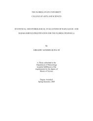
1FEBRUARY 2013 S T E F A N O V A E T A L . 843FIG. 2. Statistical moments of (a) T max and (b) T min during neutral years. Mean, standard deviation, skewness, and excess kurtosis insubpanels 1–4, respectively. Horizontal color bar applies to the skewness and excess kurtosis (subpanels 3,4).neutral states contain the remaining 30 years with 1770days. If we now make the realistic assumption that surfaceair temperature has a decorrelation time scale ofabout 3 days all over the southeastern United States(Barnston 1993), we can estimate the number of independentobservations in the ENSO and AO climateregimes as N regimein5 197 (the total number of days ineach regime, 590, divided by the decorrelation timescale of 3 days). In the neutral state there are5 590 (the total number of days in the neutralcondition, 1770, divided by the decorrelation time scale)independent records. Thus, the standard errors ofskewness and kurtosis in each climate regime areN neutralin’ 0:17 and SEregime kurt’ 0:34, respectively. Thestandard errors in the neutral phases, due to the largernumber of independent observations, are somewhatsmaller, namely, SE neutralskew ’ 0:1 andSEneutral kurt ’ 0:2. Aswe are also interested in the skewness and kurtosisdifferences between ENSO/AO regimes and neutralphases, we use the Gauss propagation of uncertaintylaw to estimate the standard errors of the differences:SE regimeskewSE regime-neutral qskew5 ffiffiffiffiffiffiffiffiffiffiffiffiffiffiffiffiffiffiffiffiffiffiffiffiffiffiffiffiffiffiffiffiffiffiffiffiffiffiffiffiffiffiffiffiffiffiffiffiffiffiffiffiffiffiffi(SE regimeskew)2 1(SE neutralqffiffiffiffiffiffiffiffiffiffiffiffiffiffiffiffiffiffiffiffiffiffiffiffiffiffiffiffiffiffiffiffiffiffiffiffiffiffiffiffiffiffiffiffiffiffiffiffiffiffiffiffiffiffiffiskew )2(SE regimekurt) 2 1(SE neutralkurt ) 2 5 0:39.5 0:19, SE regime-neutralkurt5In light of the following presentation and discussion ofskewness and kurtosis maps, the error estimates meanthat most of the non-Gaussian skewness structurespresented in this paper (regimes and regime differences)are significant at the 95% level because the amplitudesof almost all large-scale skewness features fall outsidethe 62 SE range. Most of the kurtosis patterns are alsosignificant at the 95% level, yet there are situations (i.e.,variables and regions) where the significance level goesdown to 68% (61 SE). Therefore, overall we can beconfident that the results shown here are not statisticalartifacts but represent tangible physical phenomena.3. Results and discussiona. Neutral yearsIn neutral years (for brevity, in this section, these aredefined with respect to ENSO; results for neutral yearsdefined with respect to AO are nearly identical), theexpected values of the distributions of the anomalies ofT max and T min (Figs. 2a1,b1) and T range and T ave (notshown) are all close to zero, indicating that it is unlikelythat ENSO-neutral years are biased by the presence ofan AO signal, despite the relatively larger number ofAO2 years in the ENSO-neutral regime (see Table 1).Temperature standard deviations (Figs. 2a2,b2) generallydecrease southward and are smallest in the Floridapeninsula (hereafter FP), with the exception of T min ,

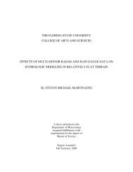
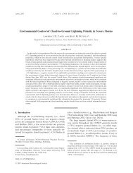
844 JOURNAL OF CLIMATE VOLUME 26whose standard deviation increases westward and isrelatively uniform in the north–south direction, althoughit is somewhat smaller in the southernmost partsof the FP. The geographic distribution of skewness variesamong the different temperature variables. Maximumtemperatures have a left (negative) skewness thatincreases southward, reaching the largest negativevalues in the FP (Fig. 2a3). In contrast, minimum temperaturesare positively skewed in the non-FP (NFP)part of the domain and negatively skewed in FP (Fig.2b3). The diurnal temperature range is weakly negativelyskewed outside of FP and weakly positivelyskewed in the FP (not shown). The daily mean temperaturehas negligible skewness with the exception ofthe FP where it has pronounced negative skewness (notshown). The geographic distribution of excess kurtosisalso varies among the four temperature variables. ForT max (Fig. 2a4) and T range (not shown) the excess kurtosisis increasingly negative to the north outside of theFP but with some positive values in the southern portionof the FP. The excess kurtosis of T min (Fig. 2b4) and T ave(not shown) is negative, with the largest values found inthe Big Bend region of Florida.The physical mechanisms responsible for the climatologicalstructure of temperature first four statisticalmoments are quite complex and mostly beyond thescope of this study. Relevant considerations should includethe climatological frequency of cloud-free skies,which increases southward (Winsberg 2003), the muchstronger impact of sea surface temperature in the FP(ibid.), and the climatological frequency and intensity ofcold and warm fronts throughout the region. Coldfrontal passage frequency generally decreases southwardto the FP (hence the larger temperature variancesto the north); however, since fronts decelerate in theirpenetration southward and frequently become stationary(Hardy and Henderson 2003), the duration offrontal-passage-related weather increases southward(DiMego et al. 1976). It takes a very strong—and thusinfrequent—arctic front to penetrate all the way to theFP, bringing very low humidities and extremely coldtemperatures (Winsberg 2003) to the area (hence theincreasingly negative skewness to the south). The diurnaltemperature range is positively correlated withthe frequency of cloudiness, precipitation, and humidity(Karl et al. 1987; Leathers et al. 1998); consequently,the largest diurnal temperature ranges are found in theFP (Leathers et al. 1998).Scatter diagrams (Fig. 3) provide a summary of thedifferences in distribution shapes of T min and T max underneutral conditions. Whether the latter are defined on thebasis of ENSO or AO makes little difference (cf. the leftand right columns of Fig. 3), which illustrates the relativerobustness of the results. With the exception of Floridastations (red circles), the standard deviations of minimumand maximum temperatures are of comparablemagnitudes, skewnesses are of comparable (and small,,0.5) magnitudes but of opposing sign (negative forT max , positive for T min ), and the kurtoses are generallysmaller for T max . For the Florida stations, on the otherhand, the standard deviation of T min is larger than that ofT max , both T min and T max are negatively skewed with theleft (negative) skewness of T min stronger than that ofT max , and the kurtosis of T max is larger than that of T min .b. ENSO phaseWe find that the ENSO phase has different effects onthe expected values of T max versus T min (Figs. 4a1,b1versus 4c1,d1): both are warmer (relative to the neutralENSO phase values) in La Niña winters, while El Niñocools T max but has a mixed effect on T min (generallycooling in FP and warming elsewhere). A likely explanationfor this is that during El Niño winters there is anincreased number of gulf storms (Eichler and Higgins2006). The air masses associated with such storms arenot particularly cold, but the increase in cloudiness(Angell 1990; Park and Leovy 2004) restricts daytimesurface warming; this same cloudiness, however, restrictsthe nighttime radiative cooling. As a result of theshifts in the distributions of T min and T max , the diurnaltemperature range increases (relative to the neutralENSO phase values) in La Niña years and decreases inEl Niño years, consistent with the relationship of diurnaltemperature range and precipitation and cloudinessdiscussed by Karl et al. (1987) and Leathers et al. (1998).The absolute values of the temperature range changeassociated with La Niña are smaller than those associatedwith El Niño. The daily mean temperatures areincreased in La Niña winters and decreased in El Niñowinters, with the effect’s magnitude being somewhatweaker in the latter.The standard deviation of T max and T min (Figs. 4a2,b2,c2,d2) and T ave (not shown) is increased in La Niña yearsand reduced in El Niño years for the northern portionsof the domain with the amplitude of the response beingstronger during El Niño. Interestingly, both El Niño andLa Niña years see a reduction of standard deviation forthese variables over the FP. The diurnal temperaturerange standard deviation is not affected by the ENSOphase in any systematic way.The magnitude of negative skewness for T max is reducedin FP in El Niño years and increased in much ofthe domain in La Niña years (Figs. 4a3,b3). For T min(Figs. 4c3,d3) the results are similar, except that the LaNiña effect is more confined to the FP. This is also reflectedin the daily averages. The skewness of the diurnal

1FEBRUARY 2013 S T E F A N O V A E T A L . 845FIG. 3. Relationship between the T min and T max (top) standard deviation, (middle) skewness, and (bottom) kurtosisfor the neutral state defined based on (left) ENSO and (right) AO. Stations in Florida are represented by red circles.

846 JOURNAL OF CLIMATE VOLUME 26FIG. 4. Difference between the means, standard deviations, skewnesses, and kurtoses (subpanels 1–4, respectively) of (a) T max of LaNiña, (b) T max of El Niño, (c) T min of La Niña, and (d) T min of El Niño vs neutral years. Small color bars apply to the mean (subpanel 1); thelarge color bar applies to the standard deviation, skewness, and excess kurtosis (subpanels 2–4).temperature range does not respond to the ENSO phasein any systematic way (not shown).The north–south gradient of the kurtosis of T max inneutral years is exacerbated in La Niña years and reducedin El Niño years (Figs. 4a4,b4). The distribution ofT min is sharpened in the northern parts of the domain (tothe point of becoming sharper than Gaussian) during ElNiño years (Figs. 4c4,d4). The T min kurtosis is also increasedin the FP during La Niña years and decreased inEl Niño years. The kurtosis of T range is generally reducedin El Niño years and is not systematically affected in LaNiña years (not shown). In La Niña years, the behaviorof T ave kurtosis is similar to that of T min , while in El Niñoyears it is similar to that of T max . In terms of absolute

1FEBRUARY 2013 S T E F A N O V A E T A L . 847FIG. 5. As in Fig. 4 but for (a) AO1, (b) AO2, (c) AO1, and (d) AO2 vs neutral years.values, El Niño affects the kurtoses of T min and T avemore than La Niña does.c. AO phaseThe expected values of T max , T min (Figs. 5a1,b1,c1,d1),T range , and T ave (not shown) are increased in AO1 anddecreased in AO2, thelatterwiththeexceptionofT range , which does not have a uniform response to AO2.The standard deviations of T max , T min (Figs. 5b2,c2), andT ave are decreased in AO1 and increased in AO2 (withthe exception of the FP where the standard deviation ofT min is decreased in both cases). The standard deviationof T range does not have a uniform response to the AOphase. The skewness anomaly of T max (Figs. 5a3,b3) andT ave is negative during AO1 and positive during AO2;for T min (Figs. 5c3,d3) and T range , the effect of AO phaseon skewness is minimal. The T max kurtosis (Fig. 5a4)is increased in much of the domain and especially in

848 JOURNAL OF CLIMATE VOLUME 26Florida during AO1. During AO2 (Fig. 5b4), stationsfarther north exhibit increased kurtosis, while those inthe FP have flattened distributions. The sharpening ofdistributions outside Florida and flattening in the FPduring AO2, as well as the sharpening of distributionsin the FP, are also seen in T min (Figs. 5c4, d4), T range ,and T ave .d. DiscussionThe warmest winters on record are frequently—butnot always—associated with either a positive AO phaseor with La Niña [see the years superscripts in Table 1,indicating the ranking of the 10 warmest and coldestJanuary–February years between 1960 and 2009 for theU.S. Southeast, based on data from the NCDC (http://www7.ncdc.noaa.gov/CDO/cdo)]. Similarly, the coldestyears are frequently—but not always—associated witha negative AO phase or with El Niño (subscripts inTable 1). Still, 40% of the extreme warm/cold yearsoccur during years that are neutral with respect to bothAO and ENSO.Our results indicate that the ENSO effect on averagetemperatures is primarily manifested through shifts inthe expected values of the daily temperature maxima.The spatial distribution of the expected value shifts isstrongly reminiscent of the precipitation anomaly distributionassociated with La Niña/El Niño phases, suggestingthat the driving mechanism behind the T maxresponse is the corresponding decrease/increase ofcloudiness that suppresses/promotes daytime radiativewarming of the surface temperatures. Daily minimumtemperatures are affected to a lesser degree, suggestingthat the El Niño–related increase in cloudiness promotesthe suppression of nighttime radiational coolingthat partially compensates for the cooling of daytimetemperatures. In contrast, the AO effect on averagetemperatures is manifested through evenly matchedshifts in both minimum and maximum temperatures.This can be explained by the fact that changes in the AOphase, unlike changes in the ENSO phase, are directlyrelated to the frequency of high-latitude frontal systemspenetrating into the Southeast. The surface temperaturechanges brought about by such systems are associatedwith the advection into the area of very cold air insteadof with cloudiness-dominated radiative effects. It shouldbe noted, however, that, despite the much stronger AO(compared to ENSO) signal in the surface temperaturesin the Southeast, it is of lesser practical consequencebecause the predictability of AO, unlike that of ENSO,is limited.In addition to shifts in the expected values of the dailyminimum and maximum surface temperatures, ourstudy demonstrates that there are statistically significantlarge-scale changes in the higher moments of the temperaturedistributions that may affect the likelihood ofexperiencing extreme cold outbreaks. For example, insouthern Alabama and the FP, La Niña winters (whichare, on average, warmer than neutral) manifest increasedstandard deviation, increased negative skewness, andincreased kurtosis of daily maximum temperatures. Increasednegative skewness and increased kurtosis areseen in the warm regimes (AO1 and La Niña) for bothT min and T max in the FP. These increases translate intothicker and longer left tails of the distributions and,therefore, into a relatively high likelihood of experiencingtemperatures significantly colder than the expected(warm) value (see Figs. 1b1,b3 for a visualillustration). The use of station (as opposed to gridded)data in the present study makes it possible to fully appreciatethe statistically significant specific behavior ofpeninsular Florida’s temperatures compared to the remainderof the Southeast.4. SummaryOur analysis confirms that the distributions of winterdaily maximum and minimum temperature anomaliesare distinctly non-Gaussian. The shapes of their distributionshave coherent spatial structures, with pronouncednorth–south gradients. At most stations, thePDFs of T min and T max have distinctly different shapes.The effects of ENSO and AO on daily minimum/maximum temperatures go beyond mere shifts in themeans—also influencing the distribution shape in a disparate,spatially coherent, and statistically significantmanner. The spatial distribution of the first four statisticalmoments for T min and T max , as well as a grosssummary of the sign of their changes under ENSO orAO regime conditions, is summarized in Table 2.In the warm regimes (La Niña and AO1) comparedto neutral, a larger effect is seen in the expected valuesof T max than of T min ;magnitudesaresimilarbetweenthe La Niña andAO1 responses. With the exceptionof the FP, the standard deviation of both T min andT max increases in La Niña, and decreases in AO1years. In both La Niña andAO1 years T max is morenegatively skewed than in neutral years over mostof the domain; the skewness of T min is unchangedexcept in south Florida. Distributions of T max aresharpened for most of the domain in AO1 years andfor Florida and the Gulf Coast in La Niña years.TheT min distributions are sharpened in south Florida forboth warm regimes.In the cold regimes (El Niño and AO2) compared toneutral, cool anomalies are seen in the expected valuesof T max for El Niño and cold anomalies in both T max and

1FEBRUARY 2013 S T E F A N O V A E T A L . 849TABLE 2. Summary of the first four statistical moments of daily maximum and minimum surface air temperatures for the Southeast inJanuary–February in neutral years, and deviations from neutral years during ENSO and AO phases. A12indicates a positive negativevalued change in the given regime relative to neutral-year values. Whenever a sign appears by itself, it applies to both Florida (FP) andnon-Florida (NFP). If only one of FP/NFP is mentioned, the change in the remaining region is negligible.Regime Variable Mean Standard deviation Skewness Excess kurtosisNeutral T max 0 Decreasing southward Negative; largestmagnitude in FPT min 0 More uniform Positive in NFP;N–S gradientnegative in FPLa Niña minusneutralEl Niño minusneutralAO1 minusneutralAO2 minusneutralT max 1 1 in NFP – 1 in FP2 in FPT min 1 1 in NFP 2 in FP 1 in FP2 in FPT max – – 1 in FP 2 in FPT min 1 in NFP – 1 in FP 1 in NFP2 in FP 2 in FPT max 1 – – 1T min 1 – 2 in FP 2 in NFP1 in FPT max – 1 1 1 in NFPT min – 1 1 in FP 1 in NFPNegative in NFP;positive in FPNegative; most negativein Florida’s Big BendT min for AO2. With the exception of Florida, thestandard deviation is strongly decreased in El Niñoyears and slightly increased in AO2 years. El Niñoreduces the negative skewness of T min and T max inFlorida; AO2 increases the positive skewness of T maxin south Florida.Let us end this paper with several thoughts on potentialutilizations and future research. The documentedvalues of the first four statistical moments atindividual stations within each regime have the potentialto be used in practical applications, such asthe generation of synthetic data for agricultural cropyields or risk assessment models. To that end, futurework is needed to develop a simple relationship betweenthe distribution statistical moments and thresholdexceedance probabilities. How could that be done?It is possible to relate the first four statistical momentsof a variable’s distribution to the probability of exceedanceof any chosen threshold values given some simpleassumptions. For example, Sura and Sardeshmuhk (2008)and Sardeshmukh and Sura (2009) developed a generalstochastic model (i.e., a null hypothesis) for the non-Gaussian statistics of weather and climate variability thathas been verified for various atmospheric and oceanicvariables (Sura 2011).In addition, if changes in the higher moments indeedalter the likelihoods of winter temperature extremes,the accurate representation of these moments should bean important consideration in the interpretation of climateand climate change modeling studies. A consequentquestion to follow up, therefore, is the extent towhich global and regional circulation models (or, forthat matter, reanalyses) are indeed capable of accuratelyrepresenting the higher moments of surface temperaturedistributions and the changes in such distributionsassociated with large-scale climate signals. This questionis addressed in a forthcoming paper.Acknowledgments. This work was partially supportedby a grant from USDA. PS was also supported throughNSF Grant AGS-0903579. The authors thank Dr. J. J.O’Brien and Mr. D. Zierden for useful discussions of theU.S. Southeast climate, and two anonymous reviewersfor their constructive comments that helped improve themanuscript.REFERENCESAngell, J. K., 1990: Variation in United States cloudiness andsunshine duration between 1950 and the drought year of 1988.J. Climate, 3, 296–308.—— and J. Korshover, 1987: Variability in U.S. cloudiness and itsrelation to El Niño. J. Climate Appl. Meteor., 26, 580–584.Attaway, J. A., 1997: A History of Florida Citrus Freezes. FloridaScience Source, Inc., 368 pp.Barnston, A. G., 1993: Atlas of Frequency Distribution: Auto-Correlation and Cross-Correlation of Daily Temperature andPrecipitation at Stations in the U.S., 1948-1991. Vol. 11.NOAA/NWS, 440 pp.Berrocal, V. J., P. F. Craigmile, and P. Guttorp, 2012: Regionalclimate model assessment using statistical upscaling anddownscaling techniques. Environmetrics, 23, 482–492.Brooks, C. E. P., and N. Carruthers, 1953: Handbook of StatisticalMethods in Meteorology. Her Majesty’s Stationery Office,412 pp.DeGaetano, A. T., and B. N. Belcher, 2007: Spatial interpolationof daily maximum and minimum air temperature based on

850 JOURNAL OF CLIMATE VOLUME 26meteorological model analyses and independent observations.J. Appl. Meteor. Climatol., 46, 1981–1992.DiMego, G. J., L. F. Bosart, and G. W. Endersen, 1976: An examinationof the frequency and mean conditions surroundingfrontal incursions into the Gulf of Mexico and Caribbean Sea.Mon. Wea. Rev., 104, 709–718.Eichler, T., and W. Higgins, 2006: Climatology and ENSO-relatedvariability of North American extratropical cyclone activity.J. Climate, 19, 2076–2093.Gershunov, A., 1998: ENSO influence on intraseasonal extremerainfall and temperature frequencies in the contiguous UnitedStates: Implications for long-range predictability. J. Climate,11, 3192–3203.——, and T. Barnett, 1998: ENSO influence on intraseasonal extremerainfall and temperature frequencies in the contiguousUnited States: Observations and model results. J. Climate, 11,1575–1586.Hagemeyer, B. C., 2006: ENSO, PNA and NAO scenarios for extremestorminess, rainfall and temperature variability duringthe Florida dry season. Preprints, 18th Conf. on Climate Variabilityand Change, Atlanta, GA, Amer. Meteor. Soc., P2.4.[Available online at http://ams.confex.com/ams/pdfpapers/98077.pdf.]Hansen, J. W., J. W. Jones, C. F. Kiker, and A. W. Hodges, 1999: ElNiño–Southern Oscillation impacts on winter vegetable productionin Florida. J. Climate, 12, 92–102.Hardy, J. W., and K. G. Henderson, 2003: Cold front variability inthe southern United States and the influence of atmosphericteleconnection patterns. Phys. Geogr., 24, 120–137.Higgins, R. W., A. Letmaa, and V. E. Kousky, 2002: Relationshipsbetween climate variability and winter temperature extremesin the United States. J. Climate, 15, 1555–1572.Huth, R., J. Kysely, and M. Dubrovsky, 2001: Time structure ofobserved, GCM-simulated, downscaled, and stochasticallygenerated temperature series. J. Climate, 14, 4047–4061.Janoviak, J. E., G. D. Bell, and M. Chelliah, 1999: A Gridded DataBase of Daily Temperature Maxima and Minima for theConterminous United States: 1948-1993. Vol. 6. NOAA/NWS,50 pp.Kalnay, E., and Coauthors, 1996: The NCEP/NCAR 40-Year ReanalysisProject. Bull. Amer. Meteor. Soc., 77, 437–471.Karl, T. R., G. Kukla, and J. Gavin, 1987: Recent temperaturechanges during overcast and clear skies in the United States.J. Climate Appl. Meteor., 26, 698–711.Kennedy, A. J., M. L. Griffin, S. L. Morey, S. R. Smith, andJ. J. O’Brien, 2007: Effects of El Niño–Southern Oscillationon sea level anomalies along the Gulf of Mexico coast.J. Geophys. Res., 112, C05047, doi:10.1029/2006JC003904.Kiladis, G. N., and H. F. Diaz, 1989: Global climatic anomaliesassociated with extremes in the Southern Oscillation. J. Climate,2, 1069–1090.Leathers, D. J., M. A. Palecki, D. A. Robinson, and K. F. Dewey,1998: Climatology of the daily temperature range annual cyclein the United States. Climate Res., 9, 197–211.Legg, T. P., 2011: Determining the accuracy of gridded climate dataand how this varies with observing-network density. Adv. Sci.Res., 6, 195–198.Miller, K. A., 1991: Response of Florida citrus growers to thefreezes of the 1980s. Climate Res., 1, 133–144.O’Shea, T. J., C. A. Beck, R. K. Bonde, H. I. Kochman, andD. K. Odell, 1985: An analysis of manatee mortality patternsin Florida, 1976-81. J. Wildl. Manage., 49, 1–11.Park, S., and C. B. Leovy, 2004: Marine low-cloud anomalies associatedwith ENSO. J. Climate, 17, 3448–3469.Perron, M., and P. Sura, 2013: Climatology of non-Gaussian atmosphericstatistics. J. Climate, 26, 1063–1083.Rogers, J. C., and R. V. Rohli, 1991: Florida citrus freezes and polaranticyclones in the Great Plains. J. Climate, 4, 1103–1113.Ropelewski, C. F., and M. S. Halpert, 1986: North American precipitationand temperature patterns associated with the ElNiño/Southern Oscillation (ENSO). Mon. Wea. Rev., 114,2352–2362.——, and ——, 1987: Global and regional scale precipitation patternsassociated with the El Niño/Southern Oscillation. Mon.Wea. Rev., 115, 1606–1626.Rupp, A. J., B. A. Bayley, S. S. P. Shen, C. K. Lee, andB. S. Strachan, 2010: An error analysis for the hybrid griddingof Texas daily precipitation data. Int. J. Climatol., 30, 601–611.Ryoo, S.-B., W.-T. Kwon, and J.-G. Jhun, 2004: Characteristics ofwintertime daily and extreme minimum temperature overSouth Korea. Int. J. Climatol., 24, 145–160.Sardeshmukh, P. D., and P. Sura, 2009: Reconciling non-Gaussianclimate statistics with linear dynamics. J. Climate, 22, 1193–1207.Shen, S. S. P., H. Yin, K. Cannon, A. Howard, S. Chetner, andT. R. Karl, 2005: Temporal and spatial changes of the agroclimatein Alberta, Canada, from 1901 to 2002. J. Appl.Meteor., 44, 1090–1105.——, A. B. Gurung, H.-S. Oh, T. Shu, and D. R. Easterling, 2011:The twentieth century contiguous US temperature changesindicated by daily data and higher statistical moments. ClimaticChange, 109, 287–317, doi:10.1007/s10584-011-0033-9.Smith, C. A., and P. D. Sardeshmukh, 2000: The effect of ENSO onthe intraseasonal variance of surface temperatures in winter.Int. J. Climatol., 20, 1543–1557.Smith, R. A., 2007: Trends in maximum and minimum temperaturedeciles in select regions of the United States. M.S. thesis,Dept. of Meteorology, The Florida State University, 58 pp.Smith, S. R., P. M. Green, A. P. Leonardi, and J. J. O’Brien, 1998:Role of multiple-level tropospheric circulations in forcingENSO winter precipitation anomalies. Mon. Wea. Rev., 126,3102–3116.Sura, P., 2011: A general perspective of extreme events in weatherand climate. Atmos. Res., 101, 1–21.——, and P. D. Sardeshmukh, 2008: A global view on non-Gaussian SST variability. J. Phys. Oceanogr., 38, 639–647.——, M. Newman, C. Penland, and P. Sardeshmukh, 2005: Multiplicativenoise and non-Gaussianity: A paradigm for atmosphericregimes? J. Atmos. Sci., 62, 1391–1409.Tencer, B., M. Rusticucci, P. Jones, and D. Lister, 2011: A southeasternSouth American daily gridded dataset of observedsurface minimum and maximum temperature for 1961–2000.Bull. Amer. Meteor. Soc., 92, 1339–1346.Toth, Z., and T. Szentimrey, 1990: The binormal distribution: Adistribution for representing asymmetrical but normal-likeweather elements. J. Climate, 3, 128–137.Winsberg, M. D., 2003: Florida Weather. University Press ofFlorida, 240 pp.Wolter, K., and M. S. Timlin, 1993: Monitoring ENSO in COADSwith a seasonally adjusted principal component index. Proc.17th Climate Diagnostics Workshop, Norman, OK, NOAA/NMC/CAC, 52–57.——, R. M. Dole, and C. A. Smith, 1999: Short-term climate extremesover the continental United States and ENSO. Part I:Seasonal temperatures. J. Climate, 12, 3255–3272.