Sensor Fusion and Calibration of Inertial Sensors, Vision, Ultra - Xsens

Linköping studies in science and technology. Dissertations.
No. 1368
Sensor Fusion and Calibration of
Inertial Sensors, Vision,
Ultra-Wideband and GPS
Jeroen Hol
Department of Electrical Engineering
Linköping University, SE–581 83 Linköping, Sweden
Linköping 2011

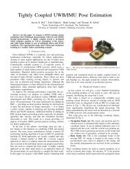
Cover illustration: A selection of Xsens devices used in this theses. From left to
right: an MTi OEM, an MTx, an MTi with uwb transmitter and an MTi-G.
Linköping studies in science and technology. Dissertations.
No. 1368
Sensor Fusion and Calibration of Inertial Sensors, Vision, Ultra-Wideband and
GPS
Jeroen Hol
hol@isy.liu.se
www.control.isy.liu.se
Division of Automatic Control
Department of Electrical Engineering
Linköping University
SE–581 83 Linköping
Sweden
ISBN 978-91-7393-197-7 ISSN 0345-7524
Copyright © 2011 Jeroen Hol
Printed by LiU-Tryck, Linköping, Sweden 2011

To Nantje!

Abstract
The usage of inertial sensors has traditionally been confined primarily to the aviation
and marine industry due to their associated cost and bulkiness. During the
last decade, however, inertial sensors have undergone a rather dramatic reduction
in both size and cost with the introduction of micro-machined electromechanical
system (mems) technology. As a result of this trend, inertial sensors
have become commonplace for many applications and can even be found in many
consumer products, for instance smart phones, cameras and game consoles. Due
to the drift inherent in inertial technology, inertial sensors are typically used in
combination with aiding sensors to stabilize and improve the estimates. The need
for aiding sensors becomes even more apparent due to the reduced accuracy of
mems inertial sensors.
This thesis discusses two problems related to using inertial sensors in combination
with aiding sensors. The first is the problem of sensor fusion: how to combine
the information obtained from the different sensors and obtain a good estimate
of position and orientation. The second problem, a prerequisite for sensor
fusion, is that of calibration: the sensors themselves have to be calibrated and provide
measurement in known units. Furthermore, whenever multiple sensors are
combined additional calibration issues arise, since the measurements are seldom
acquired in the same physical location and expressed in a common coordinate
frame. Sensor fusion and calibration are discussed for the combination of inertial
sensors with cameras, ultra-wideband (uwb) or global positioning system
(gps).
Two setups for estimating position and orientation in real-time are presented
in this thesis. The first uses inertial sensors in combination with a camera; the
second combines inertial sensors with uwb. Tightly coupled sensor fusion algorithms
and experiments with performance evaluation are provided. Furthermore,
this thesis contains ideas on using an optimization based sensor fusion method
for a multi-segment inertial tracking system used for human motion capture as
well as a sensor fusion method for combining inertial sensors with a dual gps
receiver.
The above sensor fusion applications give rise to a number of calibration problems.
Novel and easy-to-use calibration algorithms have been developed and
tested to determine the following parameters: the magnetic field distortion when
an inertial measurement unit (imu) containing magnetometers is mounted close
to a ferro-magnetic object, the relative position and orientation of a rigidly connected
camera and imu, as well as the clock parameters and receiver positions of
an indoor uwb positioning system.
v

Populärvetenskaplig sammanfattning
Användningen av tröghetssensorer har traditionellt varit begränsad främst till
marin- och flygindustrin på grund av sensorernas kostnad som storlek. Under
det senaste decenniet har tröghetssensorer storlek såväl som kostand genomgått
en dramatisk minskning tack vara införandet av micro-machined electromechanical
system (mems) teknik. Som ett resultat av denna trend, har de blivit vanliga
i många ny tillämpningar och kan nu även hittas i många konsumentprodukter,
till exempel smarta telefoner, kameror och spelkonsoler. På grund av sin drift
används tröghetssensorer vanligtvis i kombination med andra sensorer för att
stabilisera och förbättra resultatet. Behovet av andra sensorer blir ännu mer uppenbart
på grund av minskad noggrannhet hos tröghetssensorer av mems-typ.
Denna avhandling diskuterar två problem relaterade till att använda tröghetssensorer
i kombination med andra sensorer. Det första problemet är sensorfusion:
hur kombinerar man information från olika sensorer för att få en bra skattning
av position och orientering. Det andra problemet, en förutsättning för sensorfusion,
är kalibrering: sensorerna själva måste vara kalibrerade och ge mätningar
i kända enheter. När flera sensorer kombineras kan ytterligare kalibreringsproblem
uppstå, eftersom mätningarna sällan utförs på samma fysiska position eller
uttrycks i ett gemensam koordinatsystem. Sensorfusion och kalibrering diskuteras
för kombinationen av tröghetssensorer med kameror, ultra-wideband (uwb)
eller global positioning system (gps).
Två tillämpningar för att skatta läge och orientering i realtid härleds och presenteras
i den här avhandlingen. Den första använder tröghetssensorer i kombination
med en kamera, den andra kombinerar tröghetssensorer med uwb. Vidare
presenteras resultaten från ett flertal experiment för att kunna utvärdera prestanda.
Dessutom innehåller denna avhandling idéer om hur man använder en optimeringsbaserad
sensorfusionsmetod för att bestämma mänsklig rörelse, samt en
sensorfusionsmetod för att kombinera tröghetssensorer med två gps-mottagare.
Ovanstående sensorfusionstillämpningar ger upphov till ett flertal kalibreringsproblem.
Nya och lättanvända kalibreringsalgoritmer har utvecklats och testats
för att fastställa följande parametrar: distorsion av magnetfältet när en inertial
measurement unit (imu) som innehåller magnetometrar är monterad nära ett
ferro-magnetiskt objekt, relativa läget och orienteringen för en kamera och imu
som är fast monterade i förhållande till varandra, samt klockparametrar och mottagarpositioner
för ett uwb positioneringssystem för inomhusbruk.
vii

Acknowledgments
I find it very hard to believe that I managed to get this far. It seems already a
long time ago that I started my PhD studies at the automatic control group in
Linköping. I received a warm welcome from Fredrik Gustafsson and Thomas
Schön, my supervisors, who invited me to Sweden. Thank you for doing so! I
really appreciate our many discussions and the frequent application of red pencil.
I really hope to continue our fruitful collaboration in the future. Furthermore
I would like to thank Lennart Ljung, Svante Gunnarsson, Ulla Salaneck,
Åsa Karmelind and Ninna Stensgård for enabling me to work in such a pleasant
atmosphere.
Furthermore I would like to thank Per Slycke, Henk Luinge and the rest of the
Xsens team for the successful collaboration over the years and for giving me the
opportunity to finish the second half of my PhD at Xsens. In my opinion, the
combination of real world problems of industry with the theoretical approach
from academia provided an excellent environment for my research.
Living in foreign country with an unknown language is always difficult in the
beginning. I would like to thank the entire control group for making learning
the Swedish language such fun. My special thanks go to David Törnqvist and
Johan Sjöberg. You introduced me to the Swedish culture, listened to my stories
and took care of distraction from work. At Xsens would like to thank my roommates
of our not-so-silent room, Arun Vydhyanathan, Manon Kok, Martin Schepers
and Raymond Zandbergen for our spontaneous research meetings about all
the aspects of life.
This thesis has been proofread by Manon Kok, Miao Zhang, Arun Vydhyanathan
and Zoran Sjanic. You kept an eye on the presentation of the material, asked
difficult questions and improved the quality a lot, which is really appreciated.
Writing the thesis would not have been so easy without the LATEX support from
Gustaf Hendeby, Henrik Tidefelt and David Törnqvist. Thank you!
Parts of this work have been supported by MATRIS (Markerless real-time Tracking
for Augmented Reality Image), a sixth framework research program within
the European Union, CADICS (Control, Autonomy, and Decision-making in Complex
Systems), a Linneaus Center funded by the Swedish Research Council (VR)
and the Strategic Research Center MOVIII, funded by the Swedish Foundation
for Strategic Research (SSF). These are hereby gratefully acknowledged.
Finally, I am grateful to my parents for their never ending support and encouragement
and to Nantje for being the love of my life. I finally have more time to
spend with you.
ix
Enschede, June 2011
Jeroen Hol

Contents
Notation xv
I Background
1 Introduction 3
1.1 Motivation . . . . . . . . . . . . . . . . . . . . . . . . . . . . . . . . 3
1.2 Problem formulation . . . . . . . . . . . . . . . . . . . . . . . . . . 5
1.3 Motivating example . . . . . . . . . . . . . . . . . . . . . . . . . . . 6
1.4 Contributions . . . . . . . . . . . . . . . . . . . . . . . . . . . . . . 7
1.5 Publications . . . . . . . . . . . . . . . . . . . . . . . . . . . . . . . 8
1.6 Outline . . . . . . . . . . . . . . . . . . . . . . . . . . . . . . . . . . 9
2 Estimation theory 11
2.1 Parameter estimation . . . . . . . . . . . . . . . . . . . . . . . . . . 11
2.2 Sensor fusion . . . . . . . . . . . . . . . . . . . . . . . . . . . . . . . 14
2.2.1 Filtering . . . . . . . . . . . . . . . . . . . . . . . . . . . . . 14
2.2.2 Smoothing . . . . . . . . . . . . . . . . . . . . . . . . . . . . 16
2.2.3 Loose and tight coupling . . . . . . . . . . . . . . . . . . . . 18
2.3 Optimization . . . . . . . . . . . . . . . . . . . . . . . . . . . . . . . 19
3 Sensors 23
3.1 Inertial measurement unit . . . . . . . . . . . . . . . . . . . . . . . 23
3.1.1 Measurement model . . . . . . . . . . . . . . . . . . . . . . 24
3.1.2 Calibration . . . . . . . . . . . . . . . . . . . . . . . . . . . . 27
3.1.3 Strapdown navigation . . . . . . . . . . . . . . . . . . . . . 28
3.1.4 Allan variance . . . . . . . . . . . . . . . . . . . . . . . . . . 28
3.2 Vision . . . . . . . . . . . . . . . . . . . . . . . . . . . . . . . . . . . 30
3.2.1 Measurement model . . . . . . . . . . . . . . . . . . . . . . 30
3.2.2 Calibration . . . . . . . . . . . . . . . . . . . . . . . . . . . . 34
3.2.3 Correspondence generation . . . . . . . . . . . . . . . . . . 35
3.3 Ultra-wideband . . . . . . . . . . . . . . . . . . . . . . . . . . . . . 36
3.3.1 Measurement model . . . . . . . . . . . . . . . . . . . . . . 37
xi

xii CONTENTS
3.3.2 Calibration . . . . . . . . . . . . . . . . . . . . . . . . . . . . 38
3.3.3 Multilateration . . . . . . . . . . . . . . . . . . . . . . . . . 39
3.4 Global positioning system . . . . . . . . . . . . . . . . . . . . . . . 39
3.4.1 Measurement model . . . . . . . . . . . . . . . . . . . . . . 40
3.4.2 Calibration . . . . . . . . . . . . . . . . . . . . . . . . . . . . 41
3.4.3 Position, velocity and time estimation . . . . . . . . . . . . 42
4 Kinematics 43
4.1 Translation . . . . . . . . . . . . . . . . . . . . . . . . . . . . . . . . 43
4.2 Rotation . . . . . . . . . . . . . . . . . . . . . . . . . . . . . . . . . 44
4.3 Time derivatives . . . . . . . . . . . . . . . . . . . . . . . . . . . . . 47
4.4 Coordinate frame alignment . . . . . . . . . . . . . . . . . . . . . . 50
II Sensor fusion applications
5 Inertial and magnetic sensors 57
5.1 Problem formulation . . . . . . . . . . . . . . . . . . . . . . . . . . 57
5.2 Orientation estimation . . . . . . . . . . . . . . . . . . . . . . . . . 58
5.3 Multi-segment system . . . . . . . . . . . . . . . . . . . . . . . . . . 60
5.4 Magnetic field calibration . . . . . . . . . . . . . . . . . . . . . . . 64
5.4.1 Calibration algorithm . . . . . . . . . . . . . . . . . . . . . . 65
5.4.2 Experiments . . . . . . . . . . . . . . . . . . . . . . . . . . . 68
6 Inertial and vision 71
6.1 Problem formulation . . . . . . . . . . . . . . . . . . . . . . . . . . 71
6.2 Pose estimation . . . . . . . . . . . . . . . . . . . . . . . . . . . . . 72
6.2.1 Sensor fusion . . . . . . . . . . . . . . . . . . . . . . . . . . 73
6.2.2 Experiments . . . . . . . . . . . . . . . . . . . . . . . . . . . 77
6.3 Relative pose calibration . . . . . . . . . . . . . . . . . . . . . . . . 84
6.3.1 Calibration algorithm . . . . . . . . . . . . . . . . . . . . . . 84
6.3.2 Experiments . . . . . . . . . . . . . . . . . . . . . . . . . . . 87
7 Inertial and uwb 93
7.1 Problem formulation . . . . . . . . . . . . . . . . . . . . . . . . . . 93
7.2 Uwb calibration . . . . . . . . . . . . . . . . . . . . . . . . . . . . . 94
7.2.1 Existing calibration algorithms . . . . . . . . . . . . . . . . 94
7.2.2 Proposed calibration algorithm . . . . . . . . . . . . . . . . 95
7.2.3 Experiments . . . . . . . . . . . . . . . . . . . . . . . . . . . 97
7.2.4 Sensitivity analysis . . . . . . . . . . . . . . . . . . . . . . . 99
7.3 Uwb multilateration . . . . . . . . . . . . . . . . . . . . . . . . . . 99
7.3.1 ℓ 1-regularization . . . . . . . . . . . . . . . . . . . . . . . . 99
7.3.2 Experiments . . . . . . . . . . . . . . . . . . . . . . . . . . . 102
7.4 Pose estimation . . . . . . . . . . . . . . . . . . . . . . . . . . . . . 103
7.4.1 Sensor fusion . . . . . . . . . . . . . . . . . . . . . . . . . . 103
7.4.2 Experiments . . . . . . . . . . . . . . . . . . . . . . . . . . . 106

CONTENTS xiii
8 Inertial and gps 111
8.1 Problem formulation . . . . . . . . . . . . . . . . . . . . . . . . . . 111
8.2 Single receiver pose estimation . . . . . . . . . . . . . . . . . . . . 112
8.2.1 Sensor fusion . . . . . . . . . . . . . . . . . . . . . . . . . . 112
8.2.2 Experiments . . . . . . . . . . . . . . . . . . . . . . . . . . . 114
8.3 Dual receiver pose estimation . . . . . . . . . . . . . . . . . . . . . 118
8.3.1 Sensor fusion . . . . . . . . . . . . . . . . . . . . . . . . . . 118
9 Concluding remarks 121
9.1 Conclusions . . . . . . . . . . . . . . . . . . . . . . . . . . . . . . . 121
9.2 Future work . . . . . . . . . . . . . . . . . . . . . . . . . . . . . . . 122
A Linear algebra 123
A.1 Matrix differentials . . . . . . . . . . . . . . . . . . . . . . . . . . . 123
A.2 Special matrices . . . . . . . . . . . . . . . . . . . . . . . . . . . . . 124
A.3 Matrix factorizations . . . . . . . . . . . . . . . . . . . . . . . . . . 125
A.4 Partial inverses . . . . . . . . . . . . . . . . . . . . . . . . . . . . . . 126
B Quaternion algebra 129
B.1 Operators and properties . . . . . . . . . . . . . . . . . . . . . . . . 129
B.2 Multiplication . . . . . . . . . . . . . . . . . . . . . . . . . . . . . . 130
B.3 Exponential and logarithm . . . . . . . . . . . . . . . . . . . . . . . 131
C Orientation conversion 133
C.1 Rotation vectors . . . . . . . . . . . . . . . . . . . . . . . . . . . . . 133
C.2 Rotation matrices . . . . . . . . . . . . . . . . . . . . . . . . . . . . 133
C.3 Euler angles . . . . . . . . . . . . . . . . . . . . . . . . . . . . . . . 134
Bibliography 135

Notation
In this thesis, scalars are denoted with lowercase letters (u, ρ), geometric vectors
with bold lowercase letters (b, ω), state and parameter vectors with bold lowercase
letters (x, θ), quaternions with lowercase letters (q, e), and matrices with
capitals (A, R). Superscripts denote rotations and in which frame a quantity is
resolved (q bn , b n ). Subscripts are used for annotations and indexing (x t, ω ie, y u).
Coordinate frames are used to denote the frame in which a quantity is resolved,
as well as to denote the origin of the frame, e.g., b n is the position of the body
frame (b-frame) expressed in the navigation frame (n-frame) and t b is the position
of the transmitter resolved in the b-frame. Furthermore, q bn , ϕ bn and R bn
are the unit quaternion, the rotation vector and the rotation matrix, respectively.
They parameterize the rotation from the n-frame to b-frame and can be used interchangeable.
More details can be found in Chapter 4.
A complete list of used abbreviations and acronyms, a list of coordinate frames,
together with a list of mathematical operators and sets can be found in the tables
on the next pages.
xv

xvi Notation
Coordinate frames and locations
Some sets
Operators
Notation Meaning
b Body frame.
c Camera frame.
e Earth frame.
ι Image frame.
i Inertial frame.
n Navigation frame.
t Transmitter location.
Notation Meaning
Z Integer numbers.
Qs Scalar quaternions.
Q1 Unit-length quaternions.
Qv Vector quaternions.
R Real numbers.
SO(3) Special orthogonal group, 3-dimensional.
S(2) Sphere, 2-dimensional.
Notation Meaning
arg max Maximizing argument.
arg min Minimizing argument.
Cov Covariance.
[ · ×] Cross product matrix.
diag Diagonal matrix.
Dx · Jacobian matrix.
d Differential operator.
· −1 Inverse.
· −T Transposed inverse.
⊗ Kronecker product.
� · �2 2-Norm.
� · �W ·
Weighted norm.
c Quaternion conjugate.
⊙ Quaternion multiplication.
· L Left quaternion multiplication.
· R Right quaternion multiplication.
tr Trace.
· T Transpose.
vec Vectorize operator.

Notation xvii
Abbreviations and acronyms
Abbreviation Meaning
i.i.d. Independently and identically distributed.
w.r.t. With respect to.
2d Two dimensional.
3d Three dimensional.
ar Augmented reality.
cad Computer aided design.
dgps Differential gps.
dof Degrees of freedom.
ekf Extended Kalman filter.
gnns Global navigation satellite system.
gps Global positioning system.
imu Inertial measurement unit.
kf Kalman filter.
kkt Karush-Kuhn-Tucker.
map Maximum a posteriori.
mems Micro-machined electromechanical system.
ml Maximum likelihood.
nlos Non line of sight.
pdf Probability density function.
pf Particle filter.
pvt Position, velocity and time.
rmse Root mean square error.
sbas Satellite-based augmentation system.
slam Simultaneous localization and mapping.
tdoa Time difference of arrival.
toa Time of arrival.
uwb Ultra-wideband.

Part I
Background

1
Introduction
This chapter gives an introduction to the thesis by briefly explaining the setting
in which the work has been carried out, presenting the contributions in view of a
problem formulation and providing some reading directions.
1.1 Motivation
Inertial sensors have been around for decades. Traditionally they have been used
in aviation and marine industry, where they are used for navigation and control
purposes. That is, the inertial sensors are used to determine the instantaneous
position and orientation of a platform. This hardware typically is very accurate
as well as rather bulky and expensive.
The introduction of micro-machined electromechanical system (mems) technology
has lead to smaller and cheaper inertial sensors, and this trend is still continuing.
Nowadays inertial sensors have become more ubiquitous and are used
in consumer applications. They can be found in cars, gaming consoles and in every
self-respecting smart-phone. Some examples of platforms containing inertial
sensors are shown in Figure 1.1.
Currently, the major disadvantage of mems components is the reduced performance
in terms of accuracy and stability, impeding autonomous navigation. As a
result, inertial sensors are typically used in combination with aiding sources. As
there is no generic solution for three dimensional (3d) tracking in general (Welch
and Foxlin, 2002), the aiding source is chosen depending on the application. Examples
of aiding sources include actual sensors such as vision, ultra-wideband
(uwb) and the global positioning system (gps). Furthermore, constraints, for
instance from bio-mechanical models, can also be used as aiding sources.
3

4 1 Introduction
(a) Airbus A380 (b) Volvo V70
(c) iPhone (d) Nintendo Wii
Figure 1.1: Examples of platforms containing inertial sensors. By courtesy
of Airbus, Volvo cars, Apple and Nintendo.
Combined with a suitable aiding source, inertial sensors form the basis for a powerful
tracking technology which has been successfully applied in a wide range
of applications. Examples include navigation of autonomous vehicles, motion
capture and augmented reality (ar), see Figure 1.2. Navigation of autonomous
vehicles, for aerial, ground or marine applications, is a more traditional application
of inertial sensors. They are used, typically in combination with gps, to
determine the real-time position and orientation of the platform. This is in turn
used in the control loop to stabilize the platform and to make sure that it follows
a predetermined path.
For motion capture applications, small inertial measurement units (imus) are
attached to body segments. Such a system can measure the orientation and relative
position of the individual segments and thereby the exact movement of a
person or an animal. In a health-care setting, this allows clinical specialists to
analyze, monitor and train the movements of a patient. Similarly, it allows athletes
to study and improve their technique. In the movie and gaming industry,
the recorded movements of an actor form the basis for special effects or game
characters.
One of the main ideas of ar is to overlay a real scene with computer generated
graphics in real-time. This can be accomplished by showing the virtual objects

1.2 Problem formulation 5
(a) Autonomous vehicles (b) Motion capture
(c) Augmented reality (ar)
Figure 1.2: Examples of applications using inertial technology. By courtesy
of Tartan Racing and Frauenhofer IGD.
on see-through head-mounted displays or superimposing them on live video imagery.
Inertial sensors combined with vision can be used to determine the position
and orientation of the camera. This knowledge is required to position and
align the virtual objects correctly on top of the real world and to ensure that they
appear to stay in the same location regardless of the camera movement.
1.2 Problem formulation
Inertial sensors are small and unobtrusive devices which are used in a wide range
of applications. However, they have to be used together with some kind of aiding
sensor. This immediately brings us to the problem of sensor fusion: how can one
combine the information from the sensors and models to obtain a good estimate
and extract all the information from the available measurements.
The second problem is frequently overlooked. Whenever multiple sensors are
combined one also has to deal with additional calibration issues. Quantities are
seldom measured at the same position and in the same coordinate frame, implying
that the alignment, the relative position and/or orientation of the sensors, has
to be determined. Sometimes this can be taken from a technical drawing, but frequently
this has to be determined in-situ from the sensor measurements. Such

6 1 Introduction
a procedure is called a calibration procedure, and has to be designed for every
combination of sensors. A good calibration is a prerequisite to do sensor fusion.
Therefore, it is very important to have simple and efficient calibration procedures,
preferable without additional hardware.
Both sensor fusion and calibration are discussed in the thesis. We focus on the
combination of inertial sensors with vision, uwb or gps. These applications are
discussed individually, starting from a common theoretical background.
1.3 Motivating example
For outdoor applications, gps is the standard choice of aiding source to combine
with inertial sensors. However, for indoor applications this not a viable option
due to problematic reception of gps signals as well as reflections. As an alternative
one can use a uwb setup. Such a system consists of a network of synchronized
receivers that track a (potentially large) number of small transmitters.
Integrating one of these transmitters with an inertial sensor results in a 6 gls-
DOF general purpose tracking system for indoor applications. The sensor unit is
shown in Figure 1.3.
Figure 1.3: An Xsens prototype sensor unit, integrating an imu and an uwb
transmitter into a single housing.
Figure 1.4 shows a comparison of the imu, uwb and the combined imu/uwb estimates.
As is clearly seen, the imu performance rapidly decreases due to drift, especially
for position and velocity. Uwb provides only position measurements; velocity
and orientation are not available. The inertial/uwb combination provides
superior estimates. It gives accurate and stable estimates of position, velocity as
well as orientation. More details can be found in Chapter 7.
The above inertial/uwb technology is commercially available as a part of MVN
Motiongrid by Xsens Technologies (Xsens Technologies, 2010).

1.4 Contributions 7
orientation [°]
position [m]
velocity [m/s]
−2 0246
2
0
−2
180
0
0 5 10 15 20 25 30 35
0 5 10 15 20 25 30 35
−180
0 5 10 15 20 25 30 35
time [s]
Figure 1.4: Position, velocity and orientation estimates. Shown are trajectories
using the imu (–), uwb (- -) and the imu/uwb combination (–).
1.4 Contributions
The main contributions of this thesis are, listed in order of appearance:
• A concise overview of inertial sensors, vision, uwb and gps and the kinematics
linking their measurements.
• The idea of applying optimization based sensor fusion methods to multisegment
inertial tracking system.
• A calibration algorithm to calibrate the magnetic field of an imu mounted
close to a ferro-magnetic object.
• The development, testing and evaluation of a real-time pose estimation system
based on sensor fusion of inertial sensors and vision.
• An easy-to-use calibration method to determine the relative position and
orientation of a rigidly connected camera and imu.
• A calibration method to determine the clock parameters and receiver positions
of a uwb positioning system.
• The development, testing and evaluation of a tightly coupled 6 degrees of
freedom (dof) tracking system based on sensor fusion of inertial sensors
and uwb.
• A sensor fusion method for combining inertial sensors and dual gps.

8 1 Introduction
1.5 Publications
Parts of this thesis have been previously published. Material on sensor fusion
using inertial sensors and vision (Chapter 6) has been published in
J. D. Hol, T. B. Schön, and F. Gustafsson. Modeling and calibration of
inertial and vision sensors. International Journal of Robotics Research,
29(2):231–244, feb 2010b. doi: 10.1177/0278364909356812.
J. D. Hol, T. B. Schön, and F. Gustafsson. A new algorithm for calibrating
a combined camera and IMU sensor unit. In Proceedings of
10th International Conference on Control, Automation, Robotics and
Vision, pages 1857–1862, Hanoi, Vietnam, Dec. 2008b. doi: 10.1109/
ICARCV.2008.4795810.
J. D. Hol, T. B. Schön, and F. Gustafsson. Relative pose calibration
of a spherical camera and an IMU. In Proceedings of 8th International
Symposium on Mixed and Augmented Reality, pages 21–24,
Cambridge, UK, Sept. 2008a. doi: 10.1109/ISMAR.2008.4637318.
F. Gustafsson, T. B. Schön, and J. D. Hol. Sensor fusion for augmented
reality. In Proceedings of 17th International Federation of Automatic
Control World Congress, Seoul, South Korea, July 2008. doi: 10.3182/
20080706-5-KR-1001.3059.
J. D. Hol. Pose Estimation and Calibration Algorithms for Vision and
Inertial Sensors. Licentiate thesis no 1379, Department of Electrical
Engineering, Linköping University, Sweden, May 2008. ISBN 978-91-
7393-862-4.
J. D. Hol, T. B. Schön, H. Luinge, P. J. Slycke, and F. Gustafsson. Robust
real-time tracking by fusing measurements from inertial and vision
sensors. Journal of Real-Time Image Processing, 2(2):149–160, Nov.
2007. doi: 10.1007/s11554-007-0040-2.
J. Chandaria, G. Thomas, B. Bartczak, K. Koeser, R. Koch, M. Becker,
G. Bleser, D. Stricker, C. Wohlleber, M. Felsberg, F. Gustafsson, J. D.
Hol, T. B. Schön, J. Skoglund, P. J. Slycke, and S. Smeitz. Real-time
camera tracking in the MATRIS project. SMPTE Motion Imaging Journal,
116(7–8):266–271, Aug. 2007a
J. D. Hol, T. B. Schön, F. Gustafsson, and P. J. Slycke. Sensor fusion for
augmented reality. In Proceedings of 9th International Conference on
Information Fusion, Florence, Italy, July 2006b. doi: 10.1109/ICIF.
2006.301604.
Inertial and uwb (Chapter 7) related publications are
J. D. Hol, T. B. Schön, and F. Gustafsson. Ultra-wideband calibration
for indoor positioning. In Proceedings of IEEE International Confer-

1.6 Outline 9
ence on Ultra-Wideband, volume 2, pages 1–4, Nanjing, China, Sept.
2010c. doi: 10.1109/ICUWB.2010.5616867.
J. D. Hol, H. J. Luinge, and P. J. Slycke. Positioning system calibration.
Patent Application, Mar. 2010a. US 12/749494.
J. D. Hol, F. Dijkstra, H. Luinge, and T. B. Schön. Tightly coupled
UWB/IMU pose estimation. In Proceedings of IEEE International
Conference on Ultra-Wideband, pages 688–692, Vancouver, Canada,
Sept. 2009. doi: 10.1109/ICUWB.2009.5288724. Best student paper
award.
J. D. Hol, F. Dijkstra, H. J. Luinge, and P. J. Slycke. Tightly coupled
UWB/IMU pose estimation system and method. Patent Application,
Feb. 2011. US 2011/0025562 A1.
Outside the scope of this thesis fall the following conference papers.
G. Hendeby, J. D. Hol, R. Karlsson, and F. Gustafsson. A graphics processing
unit implementation of the particle filter. In Proceedings of
European Signal Processing Conference, Poznań, Poland, Sept. 2007.
J. D. Hol, T. B. Schön, and F. Gustafsson. On resampling algorithms for
particle filters. In Proceedings of Nonlinear Statistical Signal Processing
Workshop, Cambridge, UK, Sept. 2006a. doi: 10.1109/NSSPW.
2006.4378824.
1.6 Outline
This thesis consists of two parts. Part I contains the background material to the
applications presented in Part II.
Part I starts with a brief introduction to the field of estimation. It provides some
notion about the concepts of parameters estimation, system identification and
sensor fusion. Chapter 3 contains sensor specific introductions to inertial sensors,
vision, uwb and gps. The measurements, calibration techniques and standard
usage for each kind of sensor are discussed. Chapter 4, on kinematics, provides
the connection between these sensors.
Part II discusses sensor fusion for a number of applications, together with associated
calibration problems. It starts with orientation estimation using standalone
imus in Chapter 5. Chapter 6 is about estimating position and orientation using
vision and inertial sensors. Pose estimation using uwb and inertial sensors is the
topic of Chapter 7. The combination of gps and inertial sensors is discussed in
Chapter 8. Finally, Chapter 9 concludes this thesis and gives possible directions
for future work.

2
Estimation theory
This chapter provides a brief introduction to the field of estimation. It provides
some notion about the concepts of parameter estimation, system identification
and sensor fusion.
2.1 Parameter estimation
In parameter estimation the goal is to infer knowledge about certain parameters
of interest from a set of measurements. Mathematically speaking, one wants
to find a function, the estimator, which maps the measurements to a parameter
value, the estimate. In statistics literature (e.g. Trees, 1968; Hastie et al., 2009)
many different estimators can be found, among which the maximum likelihood
(ml) estimator and the maximum a posteriori (map) estimator are of particular
interest.
The ml estimate is defined in the following way
ˆθ ml = arg max p(y|θ). (2.1)
θ
That is, the estimate ˆθ ml is the value of the parameter vector θ at which the
likelihood function p(y|θ) attains its maximum. Here p(y|θ) is the probability
density function (pdf) which specifies how the measurements y are distributed
when the parameter vector θ is given. Example 2.1 shows how an ml estimate
for the mean and the covariance of a Gaussian distribution is derived.
11

12 2 Estimation theory
2.1 Example: Gaussian parameter estimation
The pdf and the corresponding log-likelihood of a Gaussian random variable y
with mean µ ∈ R m and covariance Σ ∈ R m×m , Σ ≻ 0, denoted as y ∼ N (µ, Σ) is
given by
p(y|µ, Σ) = (2π) − m 2 (det Σ) − 1 2 exp � − 1 2 (y − µ)T Σ −1 (y − µ) � , (2.2a)
log p(y|µ, Σ) = − m 2 log(2π) − 1 2 log det Σ − 1 2 (y − µ)T Σ −1 (y − µ), (2.2b)
where the dependence on the parameters µ and Σ has been denoted explicitly.
Given a set of N independent samples y1:N = {yn} N n=1 drawn from y, the ml
estimate of the parameters θ = {µ, Σ} is now given as
ˆθ = arg max
θ
= arg min
θ
= arg min
θ
p(y 1:N |θ) = arg max
θ
N�
− log p(yn|θ) n=1
N m
2
log 2π + N
2
N�
p(yn|θ) n=1
1
log det Σ +
2 tr
⎛
⎜⎝ Σ−1
n=1
N�
(yn − µ)(yn − µ) T
⎞
⎟⎠
. (2.3)
Minimizing with respect to (w.r.t.) θ yields ˆθ = { ˆµ, ˆΣ} with
ˆµ = 1
N�
y
N
n,
ˆΣ = 1
N�
(yn − ˆµ)(yn − ˆµ)
N
T , (2.4)
n=1
which are the well-known sample mean and sample covariance.
The map estimate is defined in the following way
ˆθ map = arg max p(θ|y). (2.5)
θ
That is, the estimate ˆθ map is the value of the parameter θ at which the posterior
density p(θ|y) attains its maximum. Bayes’ formula expands p(θ|y) as
p(θ|y) =
p(θ, y)
p(y)
n=1
p(y|θ)p(θ)
= . (2.6)
p(y)
This implies that the map estimate can equivalently be defined as
ˆθ map = arg max p(y|θ)p(θ). (2.7)
θ
Here, p(θ) is called the prior. It models the a priori distribution of the parameter
vector θ. In case of an uninformative, uniform prior, the map estimate and
the ml estimate become equivalent. Example 2.2 shows how a map estimate for
an exponential prior is derived. Exponential priors are for instance used in the
context of ultra-wideband (uwb) positioning, see Section 7.3.

2.1 Parameter estimation 13
2.2 Example: Range measurements with outliers
Consider a set of N independent range measurements y1:N = {yn} N n=1 with Gaussian
measurement noise. Due to the measurement technique, the measurements
are occasionally corrupted with a positive offset. That is,
y n = r + d n + e n, (2.8)
where r is the range, en ∼ N (0, σ 2 ) is the measurement noise and dn ≥ 0 is a
possibly nonzero disturbance. The presence of the disturbances is taken into
account using an exponential prior with parameter λ,
⎧
⎪⎨ λ exp(−λd
p(d n) =
n),
⎪⎩ 0,
dn ≥ 0
dn < 0.
(2.9)
The map estimate of the parameter vector θ = {r, d1, . . . dN } is now given as
ˆθ = arg max
θ
p(y 1:N |θ)p(θ) = arg max
θ
N�
p(y n|r, dn)p(d n)
N� (yn − r − d
= arg min
n)
θ n=1
2
2σ 2
N�
+ λ dn (2.10)
n=1
The last step is obtained by taking the logarithm and removing some constants.
There exists no closed form solution to (2.10). However, it can be solved using
numerical optimization methods, see Section 2.3.
As an application of parameter estimation consider the topic of system identification
(Ljung, 1999, 2008). Here, one wants to identify or estimate parameters of
dynamical systems. These parameters are computed from information about the
system in the form of input and output data. This data is denoted
n=1
z 1:N = {u 1, u 2, . . . , u N , y 1, y 2, . . . , y N }, (2.11)
where {ut} N t=1 denote the input signals and {yt} N t=1 denote the output signals (measurements).
Note that the input signals are sometimes sampled at a higher frequency
than the measurements, for instance in the case of inertial sensors and
vision. In this case, some of the measurements are missing and they are removed
from the dataset.
Besides a dataset, a predictor capable of predicting measurements is required.
More formally, the predictor is a parameterized mapping g( · ) from past input
and output signals to the space of the model outputs,
ˆy t|t−1(θ) = g(θ, z 1:t−1), (2.12)
where z 1:t−1 is used to denote all the input and output signals up to time t − 1 and
θ denotes the parameters of the predictor. Many different predictor families are
described in literature (see Ljung, 1999), including black-box models and graybox
models based on physical insight.

14 2 Estimation theory
Finally, in order to compute an estimate of the parameters θ a method to determine
which parameters are best at describing the data is needed. This is accomplished
by posing and solving an optimization problem
ˆθ = arg min V (θ, z1:N ), (2.13)
θ
where V is a cost function measuring how well the predictor agrees with the
measurements. Typically, the cost function V (θ, z 1:N ) is of the form
V (θ, z 1:N ) = 1
2
N�
t=1
�y t − ˆy t|t−1(θ)� 2 Λ t , (2.14)
where Λ t is a suitable weighting matrix. Introducing the stacked normalized
prediction vector e = vec [e 1, e 2, . . . , e N ] of length N n y where
the optimization problem (2.13) can be simplified to
e t = Λ −1/2
t (y t − ˆy t|t−1(θ)), (2.15)
ˆθ = arg min e
θ
T e. (2.16)
The covariance of the obtained estimate ˆθ can be approximated as (Ljung, 1999)
Cov ˆθ = eT e �
[Dθ e]
N ny T [Dθ e] �−1 , (2.17)
where [D · ] is the Jacobian matrix, see Appendix A.1. The dataset (2.11) on which
the estimate ˆθ is based does not have to satisfy any constraint other than that it
should be informative, i.e., it should allow one to distinguish between different
models and/or parameter values (Ljung, 1999). It is very hard to quantify this
notion of informativeness, but in an uninformative experiment the predicted output
will not be sensitive to certain parameters and this results in large variances
of the obtained estimates.
2.2 Sensor fusion
Sensor fusion is about combining information from different sensor sources. It
has become a synonym for state estimation, which can be interpreted as a special
case of parameter estimation where the parameters are the state of the system
under consideration. Depending on the application, the current state or the state
evolution are of interest. The former case is called the filtering problem, the latter
the smoothing problem.
2.2.1 Filtering
In filtering applications the goal is to find an estimate of the current state given
all available measurements (Gustafsson, 2010; Jazwinski, 1970). Mathematically
speaking, one is interested in the filtering density p(x t|y 1:t), where x t is the state
at time t and the set y 1:t = {y 1, . . . , y t} contains the measurement history up to

2.2 Sensor fusion 15
time t. The filtering density is typically calculated using the recursion
p(xt|y 1:t) = p(yt|x t)p(x t|y1:t−1) ,
p(y
�
t|y1:t−1) (2.18a)
p(yt|y 1:t−1) = p(yt|x t)p(x t|y1:t−1) dxt, (2.18b)
�
p(xt|y 1:t−1) = p(xt|x t−1)p(xt−1|y1:t−1) dxt−1. (2.18c)
This filter recursion follows from Bayes’ rule (2.6) in combination with the standard
assumption that the underlying model has the Markov property
p(x t|x 1:t−1) = p(x t|x t−1), p(y t|x 1:t) = p(y t|x t). (2.19)
The conditional densities p(xt|x t−1) and p(yt|x t) are implicitly defined by the process
model and measurement model, respectively. For the nonlinear state space
model with additive noise, we have
�
xt+1 = f (xt) + wt ⇔ p(xt|x t−1) = pwt xt − f (xt−1) � , (2.20a)
�
yt = h(xt) + vt ⇔ p(yt|x t) = pvt yt − h(xt) � . (2.20b)
Here p wt and p vt denote the pdfs of the process noise w t and the measurement
noise v t respectively. In Example 2.3, the well-known Kalman filter (kf) is derived
from the filter equations (2.18).
2.3 Example: The Kalman filter (kf)
Consider the following linear state-space model with additive noise,
x t+1 = A tx t + w t, (2.21a)
y t = C tx t + v t, (2.21b)
where w t ∼ N (0, Σ w) and v t ∼ N (0, Σ v) are independently and identically distributed
(i.i.d.) Gaussian variables. In this case (2.18) can be evaluated analytically,
resulting in the kf (Kalman, 1960; Kailath et al., 2000; Gustafsson, 2010).
Starting from a Gaussian estimate p(xt|y 1:t) = N ( ˆx t|t, Σt|t), the process model
(2.21a) gives the following joint pdf
�� � �
ˆxt|t Σt|t Σ
p(xt, xt+1|y1:t) = N ,
t|tA
At ˆx t|t
T t
AtΣt|t AtΣt|tA T t + Σ ��
. (2.22)
w
Evaluating (2.18c), i.e. marginalizing (2.22) w.r.t. xt, now yields
p(xt+1|y1:t) = N � At ˆx t|t, AtΣt|tA T � � �
t + Σw � N ˆxt+1|t, Σt+1|t . (2.23)
Similarly, the measurement model (2.21b) gives the following joint pdf
�� � �
ˆxt|t−1 Σt|t−1
p(xt, yt|y 1:t−1) = N
,
Ct ˆx t|t−1
Σt|t−1C T CtΣ t|t−1
t
CtΣ t|t−1C T t + Σ ��
.
v
(2.24)

16 2 Estimation theory
Evaluating (2.18b), i.e. marginalizing (2.24) w.r.t. xt, now yields
p(yt|y 1:t−1) = N � �
Ct ˆx t|t−1, St , (2.25)
with St = CtΣ t|t−1C T t + Σv. Evaluating (2.18a), i.e. conditioning (2.24) on yt, gives
p(xt|y 1:t) = N � ˆx t|t−1 + K t(y t − Ct ˆx t|t−1), Σt|t−1 − K tS tK T �
t
� N � �
ˆx t|t, Σt|t , (2.26)
where K t = Σ t|t−1C T t S−1
t .
Alternatively, the measurement update (2.26) can be interpreted as fusing two
information sources: the prediction and the measurement. More formally, we
have the equations
� � � �
ˆxt|t−1 I
= xt + et, et ∼ N
y t
C t
�� � � ��
0 Σt|t−1 0
,
, (2.27)
0 0 Σv from which we want to estimate x t. Ml estimation boils down to solving a
weighted least squares problem. The mean ˆx t|t and covariance Σ t|t obtained this
way can be shown to be identical to (2.26) (Humpherys and West, 2010).
To prevent the kf from being affected by faulty measurements or outliers, outlier
rejection or gating is used to discard these. The standard approach is to apply
hypothesis testing on the residuals, which are defined as
ε t = y t − ˆy t|t−1, (2.28)
i.e. the difference between the observed measurement y t and the one-step ahead
prediction from the model ˆy t|t−1 = C t ˆx t|t−1. In absence of errors, the residuals
are normal distributed as ε t ∼ N (0, S t) according to (2.25). This allows the calculation
of confidence intervals for the individual predicted measurements and
in case a measurement violates these, the measurement is considered an outlier
and is ignored.
Although conceptually simple, the multidimensional integrals in (2.18) typically
do not have an analytical solution. An important exception is the kf, discussed in
Example 2.3. However, typically some kind of approximation is used resulting in
a large family of filter types, including the extended Kalman filter (ekf) (Schmidt,
1966; Kailath et al., 2000; Gustafsson, 2010) and particle filter (pf) (Gordon et al.,
1993; Arulampalam et al., 2002; Gustafsson, 2010).
2.2.2 Smoothing
In smoothing problems, the goal is to find the best estimate of the state trajectory
given all the measurements (Jazwinski, 1970; Gustafsson, 2010). Mathematically
speaking, the posterior density p(x 1:t|y 1:t) is the object of interest, where x 1:t =
{x 1, . . . , x t} is a complete state trajectory up to time t and the set y 1:t = {y 1, . . . , y t}
contains the measurements up to time t. To obtain a point estimate from the
posterior, the map estimate is the natural choice.

2.2 Sensor fusion 17
Using the Markov property of the underlying model (2.19), it follows that the
map estimate can be expanded as
ˆx 1:t = arg max
x 1:t
p(x1:t, y1:t) = arg max p(x1) x1:t = arg min − log p(x1) −
x1:t t�
p(xi|x i−1)
i=2
t�
log p(xi|x i−1) −
i=2
t�
p(yi|x i)
i=1
t�
log p(yi|x i). (2.29)
Including (2.20) the map estimate can be formulated as the optimization problem
min
θ
�t−1
− log px1 (x1) − log pw(wi) −
i=1
i=1
t�
log pv(vi) (2.30)
i=1
s.t. x i+1 = f (x i) + w i, i = 1, . . . , t − 1
with variables θ = {x 1:t, w 1:t−1, v 1:t}.
y i = h(x i) + v i, i = 1, . . . , t
2.4 Example: Gaussian smoothing
Assuming x 1 ∼ N ( ¯x 1, Σ x1 ), w i ∼ N (0, Σ w) and v i ∼ N (0, Σ w), with known mean
and covariance, the optimization problem (2.30) simplifies using (2.2) to
min
θ
1
2 � ˜e�2 t−1
1
2 +
2
i=1
�
� ˜w i� 2 2
+ 1
2
t�
� ˜v i� 2 2
i=1
s.t. ˜e = Σ −1/2
x (x
1 1 − ¯x 1)
˜w i = Σ −1/2
w (xi+1 − f (xi)), i = 1, . . . , t − 1
˜v i = Σ −1/2
v (yi − h(xi)), i = 1, . . . , t
(2.31)
with variables θ = {x 1:t, ˜e, ˜w 1:t−1, ˜v 1:t}. The constant terms present in (2.2b) do not
affect the position of the optimum of (2.31) and have been left out. Introducing
the normalized residual vector ɛ = { ˜e, ˜w 1:t−1, ˜v 1:t}, (2.31) becomes the nonlinear
least squares problem
with variables θ = x 1:t.
min
θ
1 2 �ɛ(θ)� 2 2
(2.32)
Since map estimation is used for the smoothing problem, the problem can be
straightforwardly extended to include other parameters of interest as well. Examples
include lever arms, sensor alignment, as well as standard deviations. That is,
map estimation can be used to solve combined smoothing and calibration problems.
The filter density p(x t|y 1:t) can be obtained from the posterior density p(x 1:t|y 1:t)

18 2 Estimation theory
by marginalization,
�
p(xt|y 1:t) = p(x1:t|y 1:t) dx1:t−1, (2.33)
i.e., integrating away the variables that are not of interest, in this case the state
history x 1:t−1. This implies that the filter estimates are contained in the map
estimate of the smoothing problem. Although the smoothing problem is inherently
formulated as a batch problem, recursive versions are possible by adding
new measurements to the problem and solving the modified problem starting it
in the most recent estimate. Recent advancements in simultaneous localization
and mapping (slam) literature (Grisetti et al., 2010; Kaess et al., 2008) show that
such an approach is feasible in real-time.
2.2.3 Loose and tight coupling
In the navigation community it is not uncommon to work with so-called loosely
coupled systems. By loosely coupled approach we refer to a solution where the
measurements from one or several of the individual sensors are pre-processed
before they are used to compute the final result. A tightly coupled approach
on the other hand refers to an approach where all the measurements are used
directly to compute the final result.
As an example consider the sensor fusion of uwb and inertial sensors, see Figure
2.1. The loosely coupled approach processes the uwb measurements with a
uwb
receiver 1
receiver M
imu
gyroscopes
accelerometers
uwb
receiver 1
receiver M
imu
gyroscopes
accelerometers
position
solver
(a) Loosely coupled
(b) Tightly coupled
sensor
fusion
sensor
fusion
Figure 2.1: Two approaches to sensor fusion of uwb and inertial sensors.

2.3 Optimization 19
position solver. The positions obtained this way are used as measurements in the
sensor fusion algorithm. In a tightly coupled setup the ‘raw’ uwb measurements
are directly used in the sensor fusion algorithm.
The pre-processing step of loose coupling typically can be interpreted as some
kind of estimator, which estimates a parameter from measurements. For instance,
an ml estimator is typically used as the position solver in Figure 2.1a. The estimate
is subsequently used as an artificial measurement by the sensor fusion algorithm.
As long as the correct pdf of the estimate is used, the loose and the
tight coupled approaches become equivalent. However, this pdf is in practice
not available or approximated, resulting in a loss of information. Furthermore,
the tightly coupled approach offers additional outlier rejection possibilities, resulting
in more accurate and robust results. From a practical point of view loose
coupling might be advantageous in some cases. However, the choice for doing so
has to be made consciously and the intermediate estimates should be accompanied
with realistic covariance values.
2.3 Optimization
In Section 2.1 and Section 2.2 a number of optimization problems have been formulated.
This section aims at providing some background on how to solve these
problems.
The general form of an optimization problem is
min
θ
f (θ) (2.34a)
s.t. ci(θ) ≤ 0,
(2.34b)
c e(θ) = 0,
(2.34c)
where f is the objective function, c i are inequality constraints, c e are equality
constraints and θ are the variables. Standard algorithms for solving (2.34) exist
in optimization literature (Boyd and Vandenberghe, 2004; Nocedal and Wright,
2006), including (infeasible start) Newton methods and trust-region methods.
For the optimization problem (2.34), the first order necessary optimality conditions,
often known as the Karush-Kuhn-Tucker (kkt) conditions, are given as
(Boyd and Vandenberghe, 2004; Nocedal and Wright, 2006)
[D θ f ](θ ∗) + λ T ∗ [D θ c i](θ ∗) + ν T ∗ [D θ c e](θ ∗) = 0,
c i(θ ∗) ≤ 0,
c e(θ ∗) = 0,
λ ∗ � 0,
diag(λ ∗)c i(θ ∗) = 0,
(2.35)
where [D · ] is the Jacobian matrix, see Appendix A.1, λ and ν are the Lagrange
dual variables associated with the inequality constraints (2.34b) and with the
equality constraints (2.34c), respectively, and (θ ∗, λ ∗, ν ∗) is a candidate optimal

20 2 Estimation theory
point. Most optimization methods can be interpreted using these conditions;
given an initial guess, a local approximation is made to the kkt conditions (2.35).
Solving the resulting equations determines a search direction which is used to
find a new and improved solution. The process is then repeated until convergence
is obtained. Examples 2.5 and 2.6 provide examples relevant for this thesis.
2.5 Example: Equality constrained least squares
Consider the following equality constrained least squares problem
min
θ
1
2 �ɛ(θ)�2 2
(2.36a)
s.t. Aθ + b = 0 (2.36b)
For this problem, the first order linearization of the kkt conditions (2.35) results
in the following system of equation
� � � � � �
J T J AT ∆θ J T ɛ
= − , (2.37)
A 0 ν Aθ + b
������������������
�K
where J = D θ ɛ is the Jacobian of the residual vector ɛ w.r.t. the parameter vector
θ, and ν is the Lagrange dual variable associated with the constraint (2.36b).
Solving for (∆θ, ν) yields a primal-dual search direction, which can be used in
combination with an appropriately chosen step-size s to update the solution as
θ := θ + s∆θ.
At the optimum θ ∗ , (2.37) can be used to obtain the Jacobian
[D ɛ θ] = [D ɛ ∆θ] = −(K −1 ) 11J T . (2.38)
According the stochastic interpretation of (2.36), ɛ are normalized residuals with
a Gaussian distribution and Cov(ɛ) = I. Therefore, application of Gauss’ approximation
formula (Ljung, 1999) yields
Cov(θ) = [D ɛ θ] Cov(ɛ)[D ɛ θ] T
= (K −1 ) 11J T J(K −1 ) 11 = (K −1 ) 11. (2.39)
The last equality can be shown by expanding the (1, 1)–block of K −1 using (A.11),
(K −1 ) 11 = [I − X] (J T J) −1 , (2.40a)
X = (J T J) −1 A T � A(J T J) −1 A T � −1 A. (2.40b)
Note that (2.40) shows that the covariance of the constrained problem is closely
related to the covariance of the unconstrained problem (J T J) −1 , see also Example
2.6.

2.3 Optimization 21
2.6 Example: Constrained least squares covariance
To illustrate the covariance calculation (2.39), consider the example problem
min
θ
1
2
3�
(θk − yk) 2
k=1
s.t. θ 1 − θ 2 = 0
for which the kkt matrix K and its inverse are given by
⎡
1
0
K =
⎢⎣
0
1
0
1
0
−1
0
0
1
0
⎤
1
−1
,
0⎥⎦
0
K −1 ⎡
.5
.5
=
⎢⎣
0
.5
.5
.5
0
−.5
0
0
1
0
⎤
.5
−.5
.
0⎥⎦
−.5
The covariance of the solution is now given by the top-left 3 × 3 block of K −1 . It
is indeed correct, as can be verified by elimination of θ 1 or θ 2 and calculating
the covariance of the corresponding unconstrained problem. Furthermore, note
that the presence of the constraint results in a reduced variance compared to the
unconstrained covariance (J T J) −1 = I 3.
For an equality constrained problem, the kkt conditions (2.35) can be more compactly
written as
where the Lagrangian L is defined as
[D (θ,ν) L](θ ∗, ν ∗) = 0, (2.41)
L(θ, ν) = f (θ) + ν T c e(θ). (2.42)
Note that this interpretation can also be used for inequality constrained problems,
once the set of active constraints has been determined. Around an optimal point
(θ∗, ν∗) the Lagrangian L can be approximated as
L(θ, ν) ≈ L(θ∗, ν∗) + 1
� �T �
θ − θ∗ [Dθθ f ](θ∗) [Dθ ce] 2 ν − ν∗ T � � �
(θ∗) θ − θ∗
, (2.43)
[Dθ ce](θ∗) 0 ν − ν∗ ������������������������������������������������������������������
where the linear term is not present because of (2.41). This result can be used
to obtain the Laplace approximation (Bishop, 2006) of the pdf of (θ, ν). This
method determines a Gaussian approximation of distribution p(y) = f (y)/Z centered
on the mode y 0. The normalization constant Z is typically unknown. Taking
the Taylor expansion of − log p(y) around y 0 gives
− log p(y) ≈ − log f (y 0) + log Z + 1 2 (y − y 0) T [D yy log f (y)](y − y 0)
�K
= log a + 1 2 (y − y 0) T A(y − y 0). (2.44)
The first order term in the expansion vanishes since y 0 is a stationary point of
p(y) and therefore [D y log f (y)](y 0) = 0. Furthermore, since f is unnormalized, a

22 2 Estimation theory
cannot be determined from f (y). Taking the exponential of both sides, we obtain
p(y) ≈ a −1 exp � − 1 2 (y − y 0) T A(y − y 0) �
= (2π) − n 2 (det A) 1 2 exp � − 1 2 (y − y 0) T A(y − y 0) � = N (y 0, A −1 ). (2.45)
In the last step the normalization constant a is determined by inspection. Using
(2.43), the Laplace approximation of the pdf of (θ, ν) is given by
�� �
θ∗
p(θ, ν) ≈ N , K
ν∗ −1
�
. (2.46)
Marginalizing this result shows that the pdf of θ can be approximated as
p(θ) ≈ N � θ∗, (K −1 �
) 11 . (2.47)
This result coincides with (2.39). As the size of the problem increases, the inversion
of K can become infeasible. However, given a sparse matrix factorization of
K it is possible to efficiently calculate parts of its inverse, see Appendix A.4.
The linearized kkt system for the smoothing problem (2.32) is very sparse and
contains a lot of structure. By exploiting this structure with for instance sparse
matrix factorizations, see Appendix A.3, efficient implementations are obtained.
The work of Grisetti et al. (2010) is also of interest in this context. They exploit
the predominantly time connectivity of the smoothing problem and achieve realtime
implementations using concepts of subgraphs and hierarchies.

3
Sensors
In this thesis, inertial sensors are used in combination with aiding sensors such
as vision, ultra-wideband (uwb) or global positioning system (gps). This chapter
aims to discuss the measurements, calibration techniques and standard usage for
each kind of sensor.
3.1 Inertial measurement unit
Inertial measurement units (imus) are devices containing three dimensional (3d)
rate gyroscopes and 3d accelerometers. In many cases, 3d magnetometers are
included as well. Imus are typically used for navigation purposes where the
position and the orientation of a device is of interest. Nowadays, many gyroscopes
and accelerometers are based on micro-machined electromechanical system
(mems) technology, see Figure 3.1 and Figure 3.2.
Compared to traditional technology, mems components are small, light, inexpensive,
have low power consumption and short start-up times. Currently, their major
disadvantage is the reduced performance in terms of accuracy and bias stability.
This is the main cause for the drift in standalone mems inertial navigation
systems (Woodman, 2007). An overview of the available inertial sensor grades is
shown in Figure 3.3.
The functionality of the mems sensors is based upon simple mechanical principles.
Angular velocity can be measured by exploiting the Coriolis effect of a
vibrating structure; when a vibrating structure is rotated, a secondary vibration
is induced from which the angular velocity can be calculated. Acceleration can be
measured with a spring suspended mass; when subjected to acceleration the mass
will be displaced. Using mems technology the necessary mechanical structures
23

24 3 Sensors
mems gyroscope
mems accelerometer
Figure 3.1: A circuit board of an imu containing mems components.
Figure 3.2: Mechanical structure of a 3d mems gyroscope. By courtesy of
STMicroelectronics.
can be manufactured on silicon chips in combination with capacitive displacement
pickups and electronic circuitry (Analog Devices, 2010; STMicroelectronics,
2011).
3.1.1 Measurement model
The sensing components have one or more sensitive axes along which a physical
quantity (e.g. specific force, angular velocity or magnetic field) is converted into
an output voltage. A typical sensor shows almost linear behavior in the working
area. Based on this observation, the following (simplified) relation between the
output voltage u and the physical signal y is postulated for multiple sensors with
their sensitive axis aligned in a suitable configuration,
u t = GRy t + c. (3.1)

3.1 Inertial measurement unit 25
Cost
strategic
earth rotation rate
mems
tactical
industrial
consumer
Gyroscope bias stability [ ◦ 0.01 0.5 15 40 100
/h]
Figure 3.3: Inertial sensors grades.
Here the time dependency of the signals y and u is denoted using the subscript
t, G is a diagonal matrix containing the gain of every sensitive axis, R is the
alignment matrix specifying the direction of the sensitive axis with respect to
(w.r.t.) the sensor housing and c is the offset vector. Note that the gain and the
offset are typically temperature dependent. The calibrated measurement signal
is obtained from the measured voltages by inverting (3.1).
The sensing components in an imu are rate gyroscopes, accelerometers and magnetometers.
The gyroscopes measure angular velocity or rate-of-turn ω. The
accelerometers do not measure accelerations directly, but rather the external specific
force f . Linear acceleration ¨ b as well as the earth’s gravitational field g contribute
to the specific force. The magnetometers measure the local magnetic field
m. Both gyroscopes and accelerometers suffer from slowly time-varying biases.
In order to discuss the measurement model in more detail, a number of coordinate
frames needs to be introduced:
The body frame (b-frame) is the coordinate frame of the moving imu. Its origin
is located in the center of the accelerometer triad and it is aligned to the
casing. All the inertial measurements are resolved in this frame.
The navigation frame (n-frame) is a local geographic frame in which we want
to navigate. That is, we want to know the position and orientation of the
b-frame w.r.t. this frame. For most applications it is defined stationary w.r.t.
the earth. However, in the context of navigation over large distances it is
customary to move and rotate the n-frame along the surface of the earth.
The first definition is used throughout this thesis, unless mentioned explicitly.

26 3 Sensors
The inertial frame (i-frame) is a stationary, non-rotating frame. The imu measures
linear acceleration and angular velocity w.r.t. this frame. Its origin is
located at the center of the earth and its axis are aligned w.r.t. the stars.
The earth frame (e-frame) coincides with the i-frame, but rotates with the earth.
That is, it has its origin at the center of the earth and axes which are fixed
w.r.t. the earth.
These coordinate frames are illustrated in Figure 3.4.
t2 t1 yb xn yn z n
n
(a)
b
x b
z b
x i
x e
z i, z e
xn zn Figure 3.4: An illustration of the coordinate frames: (a) shows the b-frame
at time instants t 1 and t 2 moving w.r.t. the n-frame. (b) shows the n-frame at
latitude φ and longitude λ, the e-frame at angle α(t) = ω iet and the i-frame.
Using the notation of page xv and suppressing the time dependency of the quantities
involved, the gyroscope measurements y ω are modeled as (Titterton and
Weston, 1997)
α
λ
(b)
y ω = ω b ib + δb ω + e b ω. (3.2a)
Here, ω ib is the angular velocity of the b-frame as observed in the i-frame, δ ω
is a slowly time-varying bias and e ω is independently and identically distributed
(i.i.d.) Gaussian noise. The angular velocity can be expanded as
ω b ib = Rbn (ω n ie + ωnen) + ω b nb , (3.2b)
where R is a rotation matrix, ω ie is the earth rate, ω en is the transport rate and
ω nb is the angular velocity required for navigation purposes.
The accelerometer measurements y a are modeled as (Titterton and Weston, 1997)
y a = f b + δ b a + e b a = R bn ( ¨ b n ii − gn ) + δ b a + e b a, (3.3a)
where f is the external specific force, δ a is a slowly time-varying bias and e a is
i.i.d. Gaussian noise. The second expression in (3.3a) splits the specific force into
its contributions from the linear acceleration of the body as observed in the i-
y n
φ
y i
y e

3.1 Inertial measurement unit 27
frame ¨ b ii and the gravity vector g. The linear acceleration can be expanded as
(see Section 4.3 and (4.28)),
¨b n ii = ωn ie × ωn ie × Rni b i + 2ω n ie × ˙ b n n + ¨ b n nn, (3.3b)
where ¨ b nn is the acceleration of the body as observed in the n-frame required
for navigation purposes. In the context of navigation over large distances, it is
more common to work with the ground speed w.r.t. the earth ˙ b e instead of ˙ b n.
In this case one is interested in ¨ b en which gives rise to the following alternative
expansion of the linear acceleration (see (4.31)),
¨b n ii = ωn ie × ωn ie × Rni b i + (2ω n ie + ωn en) × ˙ b n e + ¨ b n en. (3.3c)
The centripetal acceleration terms ω n ie × ωn ie × Rni b i in (3.3b) and (3.3c) are typically
absorbed in the (local) gravity vector.
The magnetometer measurements y m are modeled as
y m = m b + e b m = R bn m n + e b m. (3.4)
Here, m is the local magnetic field vector and e m is i.i.d. Gaussian noise. In absence
of ferromagnetic objects m is the earth magnetic field and the magnetometer
measurements can be used as a compass to give the direction of the magnetic
north.
3.1.2 Calibration
Calibrating the imu boils down to finding the gain G, the alignment R and the offset
c in (3.1) for the accelerometer and the gyroscope. The calibration principle is
to subject the imu to a known acceleration or angular velocity and choose the calibration
parameters such that the observed sensor output is as likely as possible.
Ignoring the time variability of the biases and using the standard assumptions of
i.i.d. Gaussian noise, the corresponding maximum likelihood (ml) problem can
be formulated as
�
ˆθ 1
= arg min
θ t
2 �u t − h(y t, θ)� 2
Σ−1 y
, (3.5)
where the parameter vector θ = {G, R, c} consists of the parameters in (3.1) and Σ y
is the covariance of y. Traditionally, known excitations are obtained using special
manipulators such as turntables (Titterton and Weston, 1997). Alternatively, the
imu can be placed in several static orientations (Ferraris et al., 1995; Skog, 2009).
Commercially available imus are typically calibrated at production. Besides gain,
alignment and offset, temperature dependency and g-sensitivity are sometimes
also accounted for (Grewal and Andrews, 2011). The latter term describes the
effect of the specific force on the gyroscope output. Recalibration is not necessary
for the gyroscopes and the accelerometers unless the housing is opened or the
sensor is subjected to a large shock. When the imu is mounted on a ferromagnetic
object, the magnetometers do have to be recalibrated as discussed in Section 5.4.

28 3 Sensors
3.1.3 Strapdown navigation
The measurements from the accelerometers and the gyroscopes can be used to
compute the position and orientation of an object relative to a known starting
point using inertial navigation (Chatfield, 1997; Titterton and Weston, 1997). In a
strapdown configuration such as the sensor unit, the measurements are resolved
in the b-frame, rather than in the i-frame. Hence, the orientation qnb , see Section
4.2, can be calculated by integrating the angular velocity ωb nb . The position
bn can be obtained by double integration of the linear acceleration ¨ bn . This acceleration
is obtained from the external specific force f b , after it has been rotated to
the n-frame and corrected for gravity and Coriolis effects. This procedure is illustrated
in Figure 3.5. For good integration results, the initial conditions have to be
determined accurately. This is a challenging problem by itself. In practice, the
ω b nb
�
q nb
� �
f remove
rotate
gravity
b f n b¨ n b˙ n bn Figure 3.5: Strapdown inertial navigation algorithm for calculating position
and orientation from angular velocity and specific force.
angular velocity ω b nb and the external specific force f b are obtained from the gyroscope
and the accelerometer measurements. These include bias and noise terms
which cause errors in the calculated position and orientation. This so-called integration
drift is inherent to all inertial navigation. Moreover, using mems inertial
sensors, the integration drift is relatively large. Hence, the orientation estimates
and especially the position estimates are only accurate and reliable for a short
period of time.
3.1.4 Allan variance
The performance of imus is typically specified in terms of their Allan variance
(IEEE Std 1559, 2009; El-Sheimy et al., 2008). This is a time-domain analysis
method of the stochastic process of the sensor measurements which investigates
the errors as a function of averaging times.
Assume that y1:K = {yk} K k=1 is a dataset of K consecutive measurements recorded
with sample time T . The measurement is performed in a stable climate without
exciting the system. Averaging over clusters of n samples, with a cluster time
Tc = nT , we obtain ¯y 1:L(n) = { ¯y l} L l=1 , where L = ⌊ K n ⌋ and the cluster average ¯y l is

3.1 Inertial measurement unit 29
defined as
¯y l = 1
n
n�
y (l−1)n+k. (3.6)
The Allan variance for cluster time T c = nT is now defined as
σ 2 (T c) =
k=1
1 �L−1
( ¯y l+1 − ¯y
2(L − 1)
l) 2 . (3.7)
That is, it calculates the mean square cluster average error.
The Allan variance can be related to the power spectral density S of the measurements
y using (El-Sheimy et al., 2008)
σ 2 (T c) = 4
�∞
0
l=1
sin4 (πf Tc) S(f ) df . (3.8)
(πf T 2
c)
Hence, the Allan variance can be interpreted as the energy of the spectral density
passed through a filter. The bandwidth of the filter depends on the cluster time
T c. The Allan variance can therefore be used to identify various noise sources
present in the measurements. Typically it is presented as the Allan standard
deviation σ(T c) versus cluster time T c in a log–log plot.
An example of an Allan variance plot is shown in Figure 3.6. It shows the charac-
Allan standard deviation [°/hr]
10 4
10 2
10 0
10 −2
10 −2
10 −1
10 0
10 1
cluster time [s]
Figure 3.6: Allan variance for gyroscopes. Shown are results from an industrial
grade mems sensor (—) and a fiber optic sensor (—).
teristic behavior for the Allan variance for inertial sensors, where a sensor typically
has a large white noise component. This exhibits itself in the Allan variance
with a slope of − 1 2 , since averaging over a twice as long cluster will halve the
variance of the mean. However, if the cluster times increase, the bias instability
will cancel this effect and the Allan variance becomes a flat line and eventually
increases again. The quality differences between imus are mainly found in the
noise magnitude and the bias instability. Higher quality sensors, such as fiber
10 2
10 3
10 4

30 3 Sensors
optic gyroscopes, have less noise as well as improved bias stability. Less noise
results in lower Allan variance curves and improved stability results in larger
cluster times at which the Allan variance curve reaches a plateau.
The Allan variance is an easy tool to study and compare the noise characteristics
of inertial sensors. However, it does not consider factors such as linearity, temperature
stability and other calibration parameters related to dynamic accuracy.
These effects are also very relevant for sensor quality and price. Therefore, the
Allan variance should never be relied on exclusively when deciding which sensor
to use in an application.
3.2 Vision
A vision sensor is a rather complex device composed of a number of sub-systems,
as illustrated in Figure 3.7. The optical system bundles incident rays of light
and forms an analog image, which is digitized by the image sensor. Computer
vision then extracts the relevant information from the image. In this thesis we
use computer vision to extract two dimensional (2d) features in the image and
associate them to 3d points in the scene. These correspondences are considered
as the measurements from the vision system.
incident
light
objective
analog
image
image
sensor
digital camera
digital
image
Figure 3.7: The pipeline of a vision sensor.
computer
vision
correspondences
Correspondences, i.e. 2d features in the image and their associated 3d location in
the scene, are the cornerstones of many computer vision applications. They can
be classified as 2d bearings-only measurements: from the feature coordinates it
is possible to find a line on which the corresponding 3d point lies. However,
information about the distance or depth of the point is not provided. When three
or more correspondences have been obtained in a single image, they can be used
to calculate the position and orientation of the camera (Hartley and Zisserman,
2004; Ma et al., 2006).
3.2.1 Measurement model
The optical system or objective projects incident rays of light to points in the
sensor plane. Various types of objectives exist, each with a specific application
area. Examples include standard perspective lenses, wide angle lenses, zoom
lenses, macro lenses and fish-eye lenses. In general, objectives are rather complex
composite devices composed of a number of functional elements, see Figure 3.8.
The most important elements are the so-called lens elements and stops. The lens
elements have refractive surfaces which bend the light, whereas the stops limit

3.2 Vision 31
Figure 3.8: Cross section of a low-cost objective. The triplet of lens elements
bundles the parallel rays of light entering the system from the left and forms
an image on the right.
the bundle of light propagating through the system. Combining a number of
elements an optical system can be designed in such a way that the desired image
formation is achieved with minimal optical aberration.
From a pure geometric perspective, ignoring effects such as focus and lens thickness,
the process of image formation can be described as a central projection
(Hartley and Zisserman, 2004). In this projection, a ray is drawn from a point
in space toward the camera center. This ray propagates through the optical system
and intersects with the image plane where it forms an image of the point.
The perhaps best known example of a central projection is the pinhole camera,
see Figure 3.9. Its widespread use in computer vision literature can be explained
P
optical axis
zc xc optical center
c
image plane
y c
f
p vι
u ι
principal point
Figure 3.9: Pinhole camera projection. The image p of a point P is the intersection
point of the image plane and the line trough point P and the optical
center c.
by noting that a perfect perspective objective is equivalent to a pinhole camera.
To discuss the measurement model the following coordinate frames are required:
The camera frame (c-frame) is the coordinate frame of the moving camera. Its
origin is located in the optical center of the camera, with the z-axis pointing
along the optical axis.

32 3 Sensors
The image frame (ι-frame) is the 2d coordinate frame of the camera images. It
is located on the image plane, which is perpendicular to the optical axis.
According to the pinhole model the relation between an image point pι a = (u, v) T
of the analog image and its corresponding scene point pc = (X, Y , Z) T is given by
⎛ ⎞
u
λ ⎜⎝
v⎟⎠
f
=
⎛ ⎞
X
⎜⎝
Y ⎟⎠
, (3.9)
Z
where λ > 0 is a scale factor and f is the focal length. Changing from homogeneous
coordinates to Euclidean coordinates yields
� �
u
=
v
f
� �
X
. (3.10)
Z Y
This well known expression is obtained by eliminating λ from (3.9). The pinhole
projection is an ideal projection and the image formation process of a real perspective
objective will deviate from it, especially for low-quality objectives. An
example is shown in Figure 3.10. This explains why the pinhole model is typi-
(a) Observed image. (b) Corrected image.
Figure 3.10: Camera images frequently suffer from radial distortion.
cally used in combination with a compensation for radial distortion (Hartley and
Zisserman, 2004; Zhang, 2000).
Although widely used in computer vision, the pinhole camera model is only
suitable for perspective objectives with limited field of view. A more generic
model, also suitable for wide angle lenses and omnidirectional cameras, is given
by (Scaramuzza et al., 2006)
⎛ ⎞
u
λ ⎜⎝
v ⎟⎠
f (ρ)
=
⎛ ⎞
X
⎜⎝
Y ⎟⎠
, (3.11a)
Z
with λ > 0. The constant focal length has been replaced with an n-th order poly-

3.2 Vision 33
nomial of the radius ρ � √ u 2 + v 2 ,
f (ρ) �
n�
αiρ i . (3.11b)
i=0
Note that this model (3.11) includes the pinhole model (3.9) as a special case.
Furthermore, the radial distortion is already included in the model, removing the
need for a distortion compensation. To change from homogeneous coordinates to
Euclidean coordinates, we solve for λ using the last line in (3.11a). After some
algebra, one obtains
� �
u
=
v
β
r
� �
X
, (3.12a)
Y
where r � √ X2 + Y 2 and β is the positive real root of the equation
n�
αiβ i − Z
β = 0. (3.12b)
r
i=0
Finding a closed form expression for this root can be very hard and is even impossible
when n > 4. However, numerical evaluation is straightforward. A closed
form expression for the derivative is given by
∂pι a β
=
∂pc γr 3
with γ defined as
� X
Y
� �XZ Y Z −r 2 � + β
r 3
γ � Z − r
�
Y 2 −XY 0
−XY X2 �
, (3.13a)
0
n�
iαiβ i−1 . (3.13b)
i=1
This derivative is used extensively in for instance camera calibration and sensor
fusion which require gradient information to minimize the error between predicted
and measured feature positions.
Cameras deliver digital images with coordinates typically specified in pixels and
indexed from the top left corner. Furthermore, there is the possibility of nonsquare
as well as non-orthogonal pixels. These effects can be accounted for by an
affine transformation which transforms the analog image coordinates pι a = (u, v) T
into pixel coordinates pι = (x, y) T ,
� � � � � � � �
x sx sθ u x0
=
+ . (3.14)
y 0 sy v
Here, the transformation is composed of the pixel sizes s x, s y, the principal point
coordinates x 0, y 0 and a skew parameter s θ.
The camera measurements yc consist of the K correspondences {pι k ↔ pn k }K k=1
between a 2d feature in the image pι k and its corresponding 3d position in the nframe
pn k obtained using computer vision. Summarizing the previous paragraphs,
y 0

34 3 Sensors
we model the correspondences as
p ι k = P (pc k ) + eι k , (3.15)
where eι k is i.i.d. Gaussian noise. For a standard camera, the projection function P
is composed of (3.10) and (3.14), whereas for a wide angle camera P is composed
of (3.12) and (3.14). Note that P operates on pc k . As this frame is moving, the 3d
points are stored in the n-frame and the correspondences contain pn k . To express
these in the c-frame we use
p c k = Rcn (p n k − cn ), (3.16)
where R cn and c n parameterize the position and the orientation of the camera and
are called the extrinsic parameters. In contrast, the parameters in (3.9)–(3.14) are
called the intrinsic or internal parameters.
Although the models (3.9)–(3.14) are sufficient for many applications, they are
simplifications of the imaging process and have some limitations. One of these is
that the physical location of the optical center, which determines the position of
the c-frame, is not well defined. Clearly, the optical center has to lie somewhere
on the optical axis, but exactly where, or even whether it lies behind, inside, or in
front of the objective depends highly on the typically unknown detailed design
of all the elements in an objective. The location of the optical center is not of
interest in pure computer vision setting. However, it becomes important when
combining vision with inertial sensors in Chapter 6.
3.2.2 Calibration
Equations (3.9)–(3.14) contain a number of parameters which have to be determined
individually for every camera. The process of doing so is referred to as
camera calibration and is a well known problem in computer vision for which
a number of toolboxes have been developed (Zhang, 2000; Bouguet, 2003; Scaramuzza
et al., 2006). Typically, these require images at several angles and distances
of a known calibration object. A planar checkerboard pattern, see Figure
3.11, is a frequently used calibration object because it is very simple to produce
and it can be printed with a standard printer and has distinctive corners
which are easy to detect. From the images of the calibration pattern correspondences
pι k ↔ pn k are constructed. In general this is a difficult problem, but due
to the strong corners and simple planar geometry it is relatively easy to obtain
the correspondences. The required image processing is typically implemented in
off-the-shelf camera calibration software.
The goal of the calibration problem is to choose the intrinsic parameters such
that the obtained correspondences are as likely as possible. This cannot be done
without determining the extrinsic parameters of the calibration images as well.
Under the standard assumptions of i.i.d. Gaussian noise, the corresponding ml

3.2 Vision 35
Figure 3.11: A typical image used for camera calibration. The calibration
object is a planar checkerboard pattern with known dimensions.
problem can be formulated as
ˆθ = arg min
θ
K�
k=1
1
2�pι k − P ′ (p n k , θ)�22 , (3.17)
where P ′ is the projection function combining (3.15) and (3.16) and the parameter
vector θ consists of the intrinsic and extrinsic parameters. This optimization
problem can be solved using standard algorithms from nonlinear optimization
as discussed in Section 2.3. An initial guess of the parameters can be obtained
from the homographies, the one-to-one relations that exist between the images
and the planar calibration pattern (Zhang, 2000). In the remainder of this thesis,
we assume that the camera has been calibrated.
3.2.3 Correspondence generation
In general, finding the correspondences is a difficult image processing problem
where two tasks have to be solved. The first task consists of detecting points
of interest or features in the image. Here, features are distinctive elements in
the camera image, for instance, corners, edges, or textured areas. Common algorithms
include the gradient based Harris detector (Harris and Stephens, 1988),
the Laplace detector (Mikolajczyk et al., 2005), and the correlation based Kanade-
Lucas-Tomasi tracker (Shi and Tomasi, 1994).
Once a feature has been found, it needs to be associated to a known 3D point
in the scene in order to form a correspondence. This is the second task, which
can be solved using probabilistic methods such as RANSAC (Fischler and Bolles,
1981). However, it can be drastically simplified by making use of some kind of
descriptor of the feature which uniquely identifies it by providing information of

36 3 Sensors
the local image such as image patches or local histograms. This descriptor should
preferably be invariant to scale changes and affine transformations. Common
examples are SIFT (Lowe, 2004) and more recently SURF (Bay et al., 2008) and
FERNS (Ozuysal et al., 2007).
Once three or more correspondences have been obtained in a single image, they
can be used to calculate the position and orientation of the camera (Hartley and
Zisserman, 2004; Ma et al., 2006). This is actually a reduced version of the camera
calibration problem (3.17), where in this case only the extrinsic parameters are
sought as the intrinsic parameters are already known.
Correspondences can also be used to find the 3d position of a feature. In the
simplest case this can be done using the epipolar geometry of a correspondence
which is observed in two images taken from different locations. Extensions to
multiple images exist as well (Hartley and Zisserman, 2004). These are the basis
for structure from motion or bundle adjustment algorithms (Triggs et al., 2000) as
well as visual simultaneous localization and mapping (slam) applications (Davison
et al., 2007; Klein and Murray, 2007).
3.3 Ultra-wideband
Ultra-wideband (uwb) is a relatively new and promising radio technology with
applications in radar, communication and localization. It occupies a very large
frequency band, at least 0.5 GHz, as opposed to more traditional radio communications
which operate in much smaller frequency bands. Since uwb is only
allowed to transmit at very low power, see Figure 3.12, its spectrum becomes
very noise-like and it can coexist with other services without influencing them.
Power [dBm]
−40
−50
−60
−70
−80
0 2 4 6 8 10 12
Frequency [GHz]
Figure 3.12: Us uwb emission masks for indoor (–) and handheld (–) usage.
To obtain the aforementioned spectrum, uwb technology typically makes use of
impulse radio using very short pulses, typically in the order of 1 ns, resulting in a
high spatial resolution. This characteristic makes uwb very suitable for localization
applications. The localization technologies can roughly be subdivided into
three categories: systems using time, systems using angle-of-arrival and systems
using signal strength (Gezici et al., 2005; Sahinoglu et al., 2008). In this thesis we
focus on time-based methods, where position is inferred from the time it takes

3.3 Ultra-wideband 37
for a signal to travel from the transmitter to the receiver.
Among the more mature uwb applications for indoor positioning are the socalled
asset tracking systems in for instance health-care or manufacturing. Commercially
available systems (e.g. Time Domain, 2010; Ubisense, 2010) typically
consist of a network of synchronized uwb receivers which track a large number of
small, battery powered and inexpensive uwb transmitters, shown in Figure 3.13.
The position of the transmitters is determined from time of arrival (toa) mea-
Figure 3.13: Uwb hardware: a receiver (left) next to a small, mobile transmitter
(right).
surements. Reported indoor position accuracies lie in the order of decimeters
(Time Domain, 2010; Ubisense, 2010), but suffer from multipath effects and non
line of sight (nlos) conditions.
3.3.1 Measurement model
The uwb setup consists of a network of synchronized and stationary (rigidly
fixed, mounted) receivers, all taking very precise toa measurements of signals
originating from a mobile transmitter as illustrated by Figure 3.14. Although the
pulse
uwb transmitter
uwb receiver
Figure 3.14: The uwb setup consists of a number of stationary receivers
making toa measurements of signals originating from a mobile transmitter.

38 3 Sensors
receivers are synchronized to a central clock, they each have a small, constant
clock offset due to for instance cable lengths. From the time at which the signal
is transmitted it takes a while before it arrives at the receivers. Ideally, the signal
travels directly to a receiver and encounters no medium which delays and/or
attenuates it, in which case the time of flight is related to the distance traveled.
Alternatively the signal can be reflected one or more times before it is received,
also introducing a delay. The time at which the signal is transmitted is an unknown
parameter, which makes the toa measurements very similar to the gps
pseudorange measurements discussed in Section 3.4.
In summary, the toa measurement y u,m of the uwb system is the time (according
to its local clock) when receiver m receives a pulse from the transmitter. It can be
modeled as
y u,m = τ + �r n m − t n � 2 + ∆τ m + δ u,m + e u,m, (3.18)
where τ is the time of transmission of the pulse, t is the position of the transmitter,
r m is the position of the m-th receiver and ∆τ m is the clock-offset of the
m-th receiver. δ u,m ≥ 0 is a possibly nonzero delay due to nlos or multipath and
e u,m is i.i.d. Gaussian noise which is virtually independent of range. Without loss
of generality, all quantities in (3.18) are expressed in meters (using the speed of
light when necessary) and the positions are resolved in the n-frame.
3.3.2 Calibration
The toa measurements can be used to determine the position of the transmitter.
Methods for doing so are discussed in Section 3.3.3. They require a calibrated
setup; that is, they assume the positions of the receivers r m to be known in the
n-frame as well as known receiver clock offsets ∆τ m.
Although a correct calibration of the setup is a prerequisite for accurate positioning
results, it is typically taken for granted and calibration is seldom discussed.
To the best of the author’s knowledge, current calibration methods have been
developed by the hardware manufacturers and are documented in their manuals.
These methods require receiver positions and transmitter positions to be surveyed.
The surveying of positions is typically a time-consuming and error-prone
process which requires additional equipment. Such an elaborate procedure is
only feasible for permanent setups, severely limiting the deployment of a uwb
positioning system.
A major contribution of this thesis is a flexible and easy-to-use calibration algorithm
capable of calibrating a uwb setup without additional measurements and
hardware in a couple of minutes, thereby enabling flexible and portable uwb
positioning systems. It is discussed in Section 7.2, where we apply maximum
likelihood estimation to estimate the 3d receiver positions {rn m} M m=1 as well as the
receiver clock-offsets {∆τ m} M m=1 of all M receivers.

3.4 Global positioning system 39
3.3.3 Multilateration
The process of determining the transmitter position from the toa measurements
is referred to as trilateration or, more accurately, multilateration. It is a wellstudied
topic for which many algorithms are reported in literature (e.g. Chan
and Ho, 1994; Gezici et al., 2005; Sayed et al., 2005; Sahinoglu et al., 2008). The
majority of these algorithms assume ‘clean’ measurements without delays, i.e.
δ u,m = 0.
A common technique is to eliminate the time of transmission τ from (3.18) by
constructing time difference of arrival (tdoa) measurements from pairs of toa
measurements. The resulting set of hyperbolic equations can then be efficiently
solved for position. The drawback of this approach is that the constructed tdoa
measurements are no longer independently distributed which complicates the
calculations. An equivalent approach is to treat τ as an unknown and solve for
both position and time. Assuming Gaussian noise, ml estimation takes the form
of a nonlinear least squares problem,
min
t n ,τ
M�
m=1
1
2 �y u,m − τ − �r n m − t n � 2 − ∆τ m� 2
Σ−1 u
, (3.19)
where Σ u is the covariance of the toa measurements. It can be efficiently solved
using standard algorithms from nonlinear numerical optimization as discussed
in Section 2.3.
The presence of non-zero delays severely affects the accuracy of the estimated
position, giving rise to several ad hoc methods to detect which measurements
are corrupted. Typically, multilateration is performed for a number of subsets of
the measurements and the ‘best’ solution is returned. In Section 7.3 we present
a novel multilateration method based on ℓ 1 regularization which automatically
determines which measurements have a non-zero delay δ u and corrects for it.
3.4 Global positioning system
The global positioning system (gps) is a satellite-based positioning system suitable
for outdoor applications. In its basic configuration, it consists of 24 space
vehicles in 6 almost circular orbits around the earth continuously transmitting
radio signals. A user can determine its position and velocity worldwide by receiving
and decoding these signals from a number of satellites (Kaplan and Hegarty,
2006; Misra and Enge, 2006). This makes gps a specific type of global navigation
satellite system (gnns). Other systems are for instance galileo and glonas.
Gps has been operational since 1993 and is operated by the usa. Both civil and
military signals are available, where the latter are encrypted. The satellites transmit
on two frequencies, called L1 (1.6 GHz) and L2 (1.2 GHz), each using a different
code. Besides ranging signals, navigation data containing for instance the
orbit parameters of the space vehicles is transmitted. The latter data, the socalled
ephemeris data, allows the user to calculate the instantaneous position of

40 3 Sensors
the satellites and to compensate for atmospheric effects. The gps system can be
augmented using base stations broadcasting local correction terms. Differential
gps (dgps) and satellite-based augmentation system (sbas) approaches use the
information from these base stations to improve the accuracy.
Commercial receivers are available in a wide range of prices. Dual band receivers
form the high-end segment and give horizontal accuracies of 1 m in autonomous
mode (Misra and Enge, 2006). Single band receivers are nowadays available as
single chip packages and give position with a horizontal accuracy of 10 m under
good visibility (Misra and Enge, 2006). These cheap devices have opened up
many consumer applications, most notable car navigation systems.
3.4.1 Measurement model
The gps system nominally consists of 24 satellites with synchronized atomic
clocks in non-geostationary orbits around the earth. They transmit time-stamped
signals which are received by a user on earth, as illustrated by Figure 3.15. A
gps receiver
gps transmitter
signal
Figure 3.15: A gps receiver receives signals transmitted by multiple gps
satellites.
gps receiver can obtain three independent types of measurements from the received
signals (Kaplan and Hegarty, 2006; Misra and Enge, 2006): pseudorange,
Doppler and carrier phase measurements. These will be discussed below.
The code phase tracking loop in a gps receiver compares the received signal from
a satellite to a receiver generated copy. The delay between these signals is a pseudorange
measurement. After a number of standard corrections this measurement
is unambiguously related to the traveled distance as well as the receiver clock offset.
That is, the pseudorange measurement y ρ from the k-th satellite is given
by
y ρ,k = �t e k − re � 2 + ∆t + δ ρ,k + e ρ,k, (3.20)
where t k is the position of the transmitter of the k-th satellite, r is the position of
the receiver and ∆t is the receiver clock offset. Furthermore, δ ρ,k is a residual error
term resulting from e.g. uncompensated atmospheric or multipath effects and
e ρ,k is i.i.d. Gaussian noise. Without loss of generality, all quantities in (3.20) are

3.4 Global positioning system 41
expressed in meters (using the speed of light when necessary) and the positions
are resolved in the e-frame.
The relative motion between a satellite and the receiver results in a Doppler shift
of the carrier frequency. This shift is measured in the carrier tracking loop of the
receiver. After compensation for known terms, the Doppler measurement y d,k of
the k-th satellite is given by
y d,k = −(u e k )T ˙r e e + ˙
∆t + e d,k, (3.21)
where uk = �tk − r�−1 2 (tk − r) is the unit vector pointing from the receiver to
the satellite, ˙r e is the receiver velocity w.r.t. the e-frame, ∆t ˙ is the receiver clock
drift and ed,k is i.i.d. Gaussian noise. Without loss of generality, all quantities in
(3.21) are expressed in meters (using the speed of light when necessary) and the
positions and the velocities are resolved in the e-frame.
Similar to the code phase tracking loop, the carrier phase tracking loop compares
the received signal from a satellite to a receiver generated copy. The phase difference,
which can be measured very accurately, is related to the traveled distance
and an integer number of wavelengths. This makes it an ambiguous measurement,
in contrast to the pseudorange measurements. Carrier phase measurements
are typically used in a dual receiver configuration which allows for the
elimination of atmospheric and receiver clock errors. From a pair of receivers
close to each other, a and b, both observing two satellites so-called double differenced
carrier phase measurements can be formed. The double differenced carrier
phase measurement y φ,kl from the satellites k and l is given by
y φ,kl = (u e kl )T (r e a − r e b ) + λN kl + e φ,kl, (3.22)
where u kl = u k − u l is the difference of unit vectors, r is a receiver position, λ
is the wavelength, N kl ∈ Z is an integer number of carrier cycles and e φ,kl is
i.i.d. Gaussian noise. Note that correlations are introduced between measurements
with common indices due to the differencing. Without loss of generality,
all quantities in (3.22) are expressed in meters (using the speed of light when
necessary) and the positions are resolved in the e-frame. The double difference
carrier phase measurements are much more accurate than pseudorange measurements
and due to the differencing common errors are canceled. The downside is
the introduction of an integer ambiguity. This ambiguity stays constant as long
as the tracking loop does not lose track.
3.4.2 Calibration
Gps does not require any calibration by the user. All necessary parameters are
contained in the navigation data broadcast by the satellites. The gps signals are
continuously monitored by base stations and when necessary, updates are uploaded
to the satellites.

42 3 Sensors
3.4.3 Position, velocity and time estimation
In most cases, a gps receiver does not only provide measurements, but also estimates
its position, velocity and time (pvt).
The receiver position r and the receiver clock offset ∆t can be solved from the
pseudorange measurements. Assuming Gaussian noise and unbiased measurements,
i.e., δ ρ,k = 0, ml estimation takes the form of a nonlinear least squares
problem,
min
r e ,∆t
K�
k=1
1
2 �y ρ,k − �t e k − re � 2 − ∆t� 2
Σ−1 ρ
, (3.23)
where Σρ is the covariance of the pseudorange measurements. It can be efficiently
solved using standard algorithms from nonlinear numerical optimization as discussed
in Section 2.3. The accuracy of the estimates is given as
Cov
� �
ˆr e
∆t ˆ = (J T J) −1 Σρ, J =
⎡
⎢⎣
−(u e 1 )T 1
.
.
−(u e K )T 1
⎤
, (3.24)
⎥⎦
where J is evaluated at ˆr e and depends on the constellation of satellites. Using
the estimate of the receiver clock offset, the receiver clock can be synchronized
to gps time after which the time of the measurement is known. Without loss of
generality, the position estimate is typically presented as latitude, longitude and
altitude.
The receiver velocity ˙r can be solved from the Doppler measurements. Assuming
Gaussian noise, ml estimation takes the form of a least squares problem with
solution
�
ˆ˙r e �
e
∆t
ˆ˙
= (J T J) −1 J T
⎛
⎜⎝
y d,1
.
y d,K
⎞
�
ˆ˙r
, Cov
⎟⎠ e �
e
∆t
ˆ˙
= (J T J) −1 Σd, (3.25)
with J defined in (3.24). Without loss of generality, the velocity estimate is typically
presented w.r.t. a local tangent plane coordinate frame with unit vectors
pointing north, east and down, or alternatively north, west and up.

4
Kinematics
Kinematics deals with motion in absence of considerations of mass and force. It
involves assigning coordinate frames to rigid bodies and describing how these
move over time. It provides the connection between the sensors used in this
thesis.
A general, length preserving transformation between two Cartesian coordinate
frames consists of a translation and/or a rotation. These elementary transformations
are illustrated in Figure 4.1. A translation is defined as a displacement of
(a) Translation. (b) Rotation.
Figure 4.1: Elementary coordinate frame transformations.
the origin while keeping the axes aligned, whereas a rotation is a change in the
direction of the axes while keeping the origins coincident. These transformations
and their properties are the topic of this chapter.
4.1 Translation
The translation of a coordinate frame corresponds to a displacement of its origin,
while keeping the axes aligned. A point has new coordinate vectors in the
43

44 4 Kinematics
translated frame, see Figure 4.2. It follows that a point x can be expressed in the
translated u-frame using
v
x v
x
v u
x u
Figure 4.2: Translation of a coordinate frame.
u
x u � x v + v u . (4.1)
Here, x u is the position of the point x expressed in the u-frame, x v is the position
of the point x expressed in the v-frame and v u is the position of the v-frame
expressed in the u-frame. The inverse transformation is given by
x v � x u + u v , u v = −v u . (4.2)
The latter expression can be obtained from solving (4.1) for x v and comparing
the result to the definition of the inverse transformation.
4.2 Rotation
A rotation of a coordinate frame corresponds to changing the direction of the coordinate
axes, while the origin remains where it is. To introduce this concept it is
convenient to consider the active form of rotation, i.e. the rotation of a vector. To
arrive at the effect of rotating the coordinate frame, note that a counter clockwise
rotation of the coordinate frame is equivalent to a clockwise rotation of a vector.
A geometric interpretation of vector rotation is given in Figure 4.3. The point
y
v
Figure 4.3: Clockwise rotation of vector x by angle α around unit axis n.
n
α
x ∗
z
x

4.2 Rotation 45
x ∗ is obtained by a clockwise rotation of x around the unit axis n by an angle α.
Using y and z as defined in Figure 4.3, the rotation can be decomposed as
x v ∗ = y v + (z v − y v ) + (x v ∗ − z v )
= (x v · n v )n v + (x v − (x v · n v )n v ) cos α + (x v × n v ) sin α
= x v cos α + n v (x v · n v )(1 − cos α) − (n v × x v ) sin α,
where all quantities are resolved in the v-frame. This implies that a counter clockwise
rotation of the coordinate frame is given by
x u = x v cos α + n v (x v · n v )(1 − cos α) − (n v × x v ) sin α, (4.3)
where the u-frame is the rotated frame. This equation is commonly referred to as
the rotation formula or Euler’s formula (Shuster, 1993). Note that the combination
of n and α, or equivalently φ = nα is denoted as the axis-angle parameterization
or the rotation vector.
Rotations can be described using a number of different parameterizations, see
e.g. Shuster (1993) for an overview. Commonly encountered parameterizations
include rotation matrices, rotation vectors, Euler angles and unit quaternions.
Using the rotation matrix parameterization, rotations are defined as
x u � R uv x v . (4.4)
The rotation matrix R uv is a member of the special orthogonal group SO(3),
SO(3) = {R ∈ R 3×3 : RR T = I, det R = +1}. (4.5)
The inverse transformation of (4.4) is given by
x v � R vu x u , R vu = (R uv ) T . (4.6)
The latter identity is straightforwardly obtained from solving (4.4) for xv . The
equivalence between (4.3) and (4.4) can be made explicitly using some properties
of the cross product. The cross product can written as a matrix vector product,
a × b = [a×]b,
⎡
0
[a×] � ⎢⎣
a3 −a2 −a3 0
a1 ⎤
a2 −a1⎥⎦ .
0
(4.7)
Furthermore, multiple cross products can be expanded as
u × (v × w) = v(w · u) − w(u · v).
Using these relations, (4.3) can be rewritten as
x
(4.8)
u = x v cos α + n v (x v · n v )(1 − cos α) − (n v × x v ) sin α
= x v cos α + (n v × (n v × x v ) + x v )(1 − cos α) − (n v × x v ) sin α
= � I − (sin α)[n v ×] + (1 − cos α)[n v ×] 2�
x
������������������������������������������������������������������������������������������
v . (4.9)
�R uv (n v ,α)
This shows that the rotation formula (4.3) can be written in the form of (4.4). The

46 4 Kinematics
obtained matrix is identified as the rotation matrix R uv .
Euler angles define a rotation using a series of three rotations around a coordinate
axis. In case of the popular aerospace sequence, one rotates first an angle ψ about
the z-axis, then an angle θ around the y-axis and finally an angle φ around the
x-axis. Using (4.9), we obtain
R uv = R(e1, φ)R(e2, θ)R(e3, ψ)
⎡
⎤ ⎡
⎤ ⎡
⎤
1 0 0 cos θ 0 − sin θ cos ψ sin ψ 0
= ⎢⎣
0 cos φ sin φ⎥⎦
⎢⎣
0 1 0 ⎥⎦ ⎢⎣
− sin ψ cos ψ 0⎥⎦
0 − sin φ cos φ sin θ 0 cos θ 0 0 1
⎡
⎤
cos θ cos ψ cos θ sin ψ − sin θ
= ⎢⎣
sin φ sin θ cos ψ − cos φ sin ψ sin φ sin θ sin ψ + cos φ cos ψ sin φ cos θ⎥⎦
cos φ sin θ cos ψ + sin φ sin ψ cos φ sin θ sin ψ − sin φ cos ψ cos φ cos θ
.
(4.10)
Here, the convention is to call the Euler angles (φ, θ, ψ) roll, pitch and yaw or
bank, elevation and heading.
Alternatively, a rotation can be defined using unit quaternions as
x u � q uv ⊙ x v ⊙ (q uv ) c . (4.11)
Here, {xu , xv } ∈ Qv are the quaternion equivalents of {xu , xv }, quv ∈ Q1 is a unit
quaternion describing the rotation from the v-frame to the u-frame and ⊙, · c denote
quaternion multiplication and conjugation respectively. Details on quaternions
and their properties can be found in Appendix B. The inverse transformation
is given by
x v � q vu ⊙ x u ⊙ (q vu ) c , q vu = (q uv ) c . (4.12)
The latter identity can be obtained by solving (4.11) for xv and comparing the
result to the definition of the inverse transformation. The connection to (4.3) can
be made explicit by expanding the quaternion products in (4.11) and substituting
quv = (q0, q) = (cos α 2 , −nv sin α 2 ). This gives
(0, x u ) = � 0, q 2 0xv + (q · x v )q + q × (q × x v ) + 2q0(q × x v ) �
(4.13)
= � 0, (q 2 0 − q · q)xv + 2(q · x v )q + 2q0(q × x v ) �
(4.14)
= (0, x v cos α + n v (x v · n v )(1 − cos α) − (n v × x v ) sin α) . (4.15)
Note that the vector component is identical to (4.3). The relation to the rotation
matrix parameterization (4.4) is given by
x u = q uv ⊙ x v ⊙ (q uv ) c = [(q uv ) L ][(q uv ) R ] T x v �
1 01×3
=
03×1 Ruv � �
0
xv �
, (4.16)
see also Example B.2.
All rotation parameterizations describe the same quantity and can be converted
to each other, see Appendix C. They can be used interchangeably. However, there
are differences in the number of parameters, singularities, uniqueness and the dif-

4.3 Time derivatives 47
ficulty of the corresponding differential equations describing the evolution over
time. In this thesis unit quaternions are used. The rationale for doing so is that
unit quaternions give a non-singular representation with only 4 parameters. Furthermore,
they have a rather simple bilinear differential equation which can be
integrated analytically. In contrast, Euler angles and rotation vectors have only
three parameters, but have a nonlinear differential equation. Additionally, Euler
angles suffer from singularities. Rotation matrices have at least 6 parameters and
need to satisfy orthogonality constraints. Although quaternions are used for all
the calculations, rotation matrices are occasionally used to simplify notation and
give insight. Furthermore, Euler angles provide a relatively intuitive representation
which is suitable for two dimensional (2d) visualization purposes.
4.3 Time derivatives
Position and orientation are not directly measured by an inertial measurement
unit (imu). Instead the time derivatives angular velocity and acceleration are
measured, see Section 3.1. In this section these quantities are introduced and it
is shown how position and orientation can be obtained from them.
The time derivative of a rotation is given by
˙q uv = 1 2 ωu uv ⊙ q uv = q uv ⊙ 1 2 ωv uv. (4.17)
To derive this expression, note that a rotation can be decomposed into incremental
rotations (see e.g. Shuster, 1993). Hence, it is possible to decompose a timevarying
quaternion as
q uv (t + δt) = δq ⊙ q uv (t) = � cos δθ 2 , nu sin δθ �
uv
2 ⊙ q (t),
for some rotation axis n u and angle increment δθ. Differentiating this expression
with respect to (w.r.t.) time results in
˙q uv q
(t) � lim
δt→0
uv (t + δt) − quv (t)
δt
= lim
δt→0
δq − 1
δt ⊙ quv (t) = 1 2 ωu uv(t) ⊙ q uv (t).
Here, ωu uv, the instantaneous angular velocity from the v-frame to the u-frame
expressed in the u-frame, is defined as
ω u �
δθ cos 2 − 1, n
uv � 2 lim
δt→0
u sin δθ �
�
�
2
u δθ
= 0, lim n . (4.18)
δt
δt→0 δt
Note that the angular velocity ω u uv ∈ Q v, i.e., it is a vector. The second equality of
(4.17) is derived using a similar argument. From (4.17) we also obtain
˙q uv � q uv ⊙ 1 2 ωv uv
� 1 2 ωu uv ⊙ q uv = q uv ⊙ q vu ⊙ 1 2 ωu uv ⊙ q uv ,
˙q vu � q vu ⊙ 1 2 ωu vu

48 4 Kinematics
This implies that the identities
= d
dt ((quv ) c ) = ( ˙q uv ) c � ( 1 2 ωu uv ⊙ q uv ) c = q vu ⊙ − 1 2 ωu uv.
ω u uv = q uv ⊙ ω v uv ⊙ q vu , ω u uv = −ω u vu, (4.19)
can be used to change the coordinate frames of the angular velocity.
Suppose that the u-frame and the v-frame are rotated w.r.t. each other. That is,
with slight abuse of notation, position vectors are transformed as
x u = R uv x v = q uv ⊙ x v ⊙ q vu . (4.20)
Using (4.17), this expression can be differentiated to obtain
˙x u = ˙q uv ⊙ x v ⊙ q vu + q uv ⊙ x v ⊙ ˙q vu + q uv ⊙ ˙x v ⊙ q vu
= 1 2 ωu uv ⊙ q uv ⊙ x v ⊙ q vu − q uv ⊙ x v ⊙ q vu ⊙ 1 2 ωu uv + q uv ⊙ ˙x v ⊙ q vu
= ω u uv × x u + q uv ⊙ ˙x v ⊙ q vu , (4.21a)
where × is the quaternion cross product, see Appendix B.1. Since this operator
extends the vector cross product, (4.21a) is equivalent to
To avoid confusion later on, we write (4.21b) as
where ˙x u u and ˙x u v are defined according to
˙x u = ω u uv × x u + R uv ˙x v . (4.21b)
˙x u u = ω u uv × x u + ˙x u v , (4.21c)
˙x u u � d
dt xu , ˙x u v � R uv ˙x v uv d
v = R dt xv . (4.22)
The additional subscript denotes the coordinate frame in which the differentiation
is performed.
The inertial frame (i-frame), the earth frame (e-frame), the navigation frame (nframe)
and the body frame (b-frame) have been introduced in Section 3.1. The
origins of the i-frame and the e-frame coincide and the transformation between
these systems is a pure rotation given by
b i = R ie b e . (4.23)
Differentiating (4.23) twice w.r.t. time using (4.21), we obtain
˙b i i = ωi ie × bi + ˙ b i e,
¨b i ii = ˙ωi ie × bi + ω i ie × ˙ b i i + ¨ b i ei
= ω i ie × ωi ie × bi + ω i ie × ˙ b i e + ¨ b i ei . (4.24)
The last identity makes use of the fact that the angular velocity ωi ie is constant,
i.e. ˙ω i ie = 0. In many applications, the n-frame is defined stationary w.r.t. the
e-frame. That is,
b e = R en b n + n e , (4.25)

4.3 Time derivatives 49
where n e and R en are constant. Differentiation w.r.t. time gives ˙ b e e = ˙ b e n. Hence,
and ¨ bi ei as can be expanded using (4.21) as
¨b i ei
˙b i e = R ie ˙ b e e = R ie ˙ b e n = ˙ b i n, (4.26)
= d
dt ˙ b i e = d
dt ˙ b i n = d
dt (Rin ˙ b n n) = ω i ie × ˙ b i n + ¨ b i nn. (4.27)
Combining (4.24), (4.26) and (4.27) and rotating the result, we obtain
¨b n ii = ωn ie × ωn ie × Rni b i + 2ω n ie × ˙ b n n + ¨ b n nn, (4.28)
where ω n ie × ωn ie × Rni b i is known as the centrifugal acceleration and 2ω n ie × ˙ b n n as
the Coriolis acceleration. This expression transforms ¨ b n ii to ¨ b n nn. The latter can be
integrated to obtain velocity ˙ b n n and position b n :
⎧
d ⎪⎨ dt
⎪⎩
bn = ˙ b n n,
d
dt ˙ b n n = ¨ b n nn
⇒
⎧
⎪⎨
⎪⎩
b n t+1 = bnt + T ˙ b n n,t +
˙b n n,t+1 = ˙ b n n,t + T ¨ b n nn,t
T 2
2 ¨ b n nn,t,
(4.29)
The integration has been performed under the assumption that the acceleration
¨b n nn,τ is constant in the interval τ ∈ (t, t + T ).
In the context of navigation over large distances it is customary to move and rotate
the n-frame along the surface of the earth. In that case, (4.25) is not satisfied
with constant ne and Ren , so (4.26)–(4.29) are no longer valid. Instead, ¨ bi ei can be
expanded using (4.21) as
¨b i ei
= d
dt ˙ b i e = d
dt (Rin ˙ b n e ) = ω i in × ˙ b i e + ¨ b i en. (4.30)
Substituting this expression in (4.24) and rotating the result, we obtain
¨b n ii = ωn ie × ωn ie × Rni b i + (2ω n ie + ωn en) × ˙ b n e + ¨ b n en, (4.31)
since ω n in = ωn ie + ωn en. This expression transforms ¨ b n ii to ¨ b n en. The latter can be
integrated to obtain the ground speed ˙ b n e .
The orientation between the b-frame and the i-frame can be decomposed as
q ib = q ie ⊙ q en ⊙ q nb . (4.32)
Differentiating this expression w.r.t. time using (4.17) and (4.19) gives
q ib ⊙ 1 2 ωb ib = qie ⊙ 1 2 ωe ie ⊙ qen ⊙ q nb + q ie ⊙ q en ⊙ 1 2 ωn en ⊙ q nb
Comparing terms gives
+ q ie ⊙ q en ⊙ q nb ⊙ 1 2 ωn nb
= q ib ⊙ q be ⊙ 1 2 ωe ie ⊙ qeb + q ib ⊙ q bn ⊙ 1 2 ωb en ⊙ q nb
+ q ib ⊙ 1 2 ωn nb
= q ib ⊙ 1 2 (ωb ie + ωben + ω b nb ) (4.33)
ω b ib = ωb ie + ωben + ω b nb . (4.34)

50 4 Kinematics
This expression transforms ωb ib to ωb nb . The latter can be integrated to obtain the
orientation:
d
dt qnb = q nb ⊙ 1 2 ωb nb
⇒ qnb t+1 = qnb t ⊙ exp( T 2 ωb nb,t ) (4.35)
The integration has been performed under the assumption that the angular velocity
ωb nb,τ is constant in the interval τ ∈ (t, t + T ). Details on the integration of
quaternions are provided in Appendix B.3.
4.4 Coordinate frame alignment
A further topic of kinematics is the alignment of coordinate frames, that is, finding
the relative position and orientation between two coordinate frames. This
problem has received a lot of attention in the field of robotics under the name of
hand-eye calibration (Tsai and Lenz, 1989; Daniilidis, 1999; Strobl and Hirzinger,
2006). In this thesis, the problem of aligning coordinate frames occurs for instance
in the context of comparing filter performance with an external optical
reference system such as Vicon, see Figure 4.4. In this section we discuss two
cases which will be used in subsequent chapters.
navigation body
reference tool
inertial system
reference system
Figure 4.4: A reference system introduces additional coordinate frames.
Solid lines indicate rigid connections which have to be calibrated, dotted
lines are non-rigid, time varying relations.
First, consider the case of determining the relative orientation from measuring
a vector quantity in two coordinate frames, here denoted the u-frame and the
v-frame. This gives rise to the following maximum likelihood (ml) problem, see
Section 2.1,
max
θ
N�
p(e u n) + p(e v n) (4.36)
n=1
s.t. y u n = v u n + e u n, n = 1, . . . , N
y v n = R vu v u n + e v n, n = 1, . . . , N
with parameter vector θ = {R vu , {v u n, e u n, e v n} N n=1 }. Dependent on the measurement
noise, solving the general problem (4.36) can be very hard. In case of

4.4 Coordinate frame alignment 51
e u n ∼ N (0, Σ u) and e v n ∼ N (0, Σ v) with Σ u = Σ v = σ 2 I 3, we can introduce a combined
noise e n = y u n − R uv y v n = e u n − R uv e v n ∼ N (0, 2σ 2 I 3). Under this assumption
solving (4.36) is equivalent to solving
min
R uv
N�
�en� 2 2
n=1
s.t. e n = y u n − R uv y v n, n = 1, . . . , N
(4.37)
Parameterizing the orientation R uv using the unit quaternion q uv , the closed form
solution to this problem is given by Theorem 4.1.
4.1 Theorem (Relative orientation from vector measurements). Let {y u n} N n=1
and {y v n} N n=1 measurements satisfying yu n ≈ q uv ⊙ y v n ⊙ q vu . Then the sum of the
squared residuals,
V (q uv ) =
N�
�en� 2 2 =
n=1
N�
n=1
�y u n − q uv ⊙ y v n ⊙ q vu � 2 2 , (4.38)
is minimized by ˆq uv = v 1, where v 1 is the eigenvector corresponding to the largest
eigenvalue λ 1 of the system Av = λv with
A = −
N�
(y u n) L (y v n) R . (4.39)
n=1
Proof: Analogous to Horn (1987), the squared residuals can be written as
�e n� 2 2 = �yu n� 2 2 − 2yu n · (q uv ⊙ y v n ⊙ q vu ) + �y v n� 2 2 .
Minimization only affects the middle term, which can be simplified to
y u n · (q uv ⊙ y v n ⊙ q vu ) = − (y u n ⊙ (q uv ⊙ y v n ⊙ q vu )) 0
= −(y u n ⊙ q uv ) T (y v n ⊙ q vu ) c
= −(q uv ) T (y u n) L (y v n) R q uv ,
using the relation (a ⊙ b) 0 = a T b c for the scalar part of quaternion multiplication.
The minimization problem can now be restated as
arg min
�q uv � 2=1
N�
�en� 2 2
n=1
= arg max
�q uv � 2=1
(q uv ) T Aq uv ,
where A is defined in (4.39). Using (B.3),(B.19) and (B.20) we have
(y u n) L (y v n) R = [−(y u n) L ] T [−(y v n) R ] T = [(y v n) R )(y u n) L ] T = [(y u n) L (y v n) R ] T ,
from which can be concluded that A is a real symmetric matrix.
Let q uv = V α with �α� 2 = 1, where V is an orthonormal basis obtained from the

52 4 Kinematics
symmetric eigenvalue decomposition of A = V ΛV T . Then,
(q uv ) T Aq uv = α T V T V ΛV T V α =
4�
α 2 i λi ≤ λ1, where λ 1 is the largest eigenvalue of A. Equality is obtained for α = (1, 0, 0, 0) T ,
that is, ˆq uv = v 1.
A second alignment problem is to determine the relative pose from pairs of relative
pose measurements. Two closely related scenarios, both known as handeye
calibration, are described in robotics literature, see e.g. Tsai and Lenz (1989);
Strobl and Hirzinger (2006). The classical hand-eye calibration scenario is to
A n
X
v w
Z
u x
(a) AX = ZB
B n
A n
i=1
X
v’ w’
X
v w
u x
(b) AX = XB
Figure 4.5: Two versions of the hand-eye calibration problem.
move a manipulator (hand) from v to v’ and to observe this change with a sensor
(eye) which moves from w to w’, as illustrated by Figure 4.5b. Evaluating the two
routes from w’ to v yields the relation AX = XB, from which the unknown transformation
X can be solved given a number of relative poses {An, Bn} N n=1 . Instead
of working with changes in manipulator pose and sensor pose, it is possible to
use these poses directly, see Figure 4.5a. Evaluating the two routes from w to u in
this slightly more general scenario yields the relation AX = ZB, from which the
unknown transformations X and Z can be jointly solved given a number of poses
{An, Bn} N n=1 .
Expanding the AX = ZB problem, we have that the measurements {q uv
n , v u n} N n=1
and {q xw
n , w x n} N n=1
are, in absence of noise, related by
� q uv
n ⊙ q vw = q ux ⊙ q xw
n ,
v u n + R uv
n w v = x u + R ux w x n.
B n
(4.40)
This is an inherently coupled and nonlinear problem in the unknowns {q ux , x u }
and {q vw , w v }. Many nonlinear optimization approaches have been formulated
(Strobl and Hirzinger, 2006). However, assuming known orientations, the trans-

4.4 Coordinate frame alignment 53
lational part is linear in the unknowns xu and wv ,
v u n − R ux w x n = � I3 −Ruv �
n
� xu �
. (4.41)
Decoupling approaches provide a starting point for the optimization approaches
and are frequently employed directly with satisfactory results. An explicit solution
to the rotational part is given by Theorem 4.2.
4.2 Theorem (Relative orientation from orientation measurements). Suppose
{quv n } N n=1 and {qxw n } N n=1 are measurements satisfying quv n ⊙ qvw ≈ qux ⊙ qxw n . Then
the residual rotation error,
V (q ux , q vw ) =
N�
�en� 2 2 =
n=1
N�
n=1
w v
�q uv
n ⊙ q vw ⊙ q wx
n ⊙ q xu − 1� 2 2 , (4.42)
is minimized by ˆq ux = v 1 and ˆq vw = u 1, where u 1 and v 1 are the first left and
right singular vectors of the matrix A = U ΣV T , with
A =
N�
[(q uv
n=1
Proof: The residual orientation error can be rewritten as
�e n� 2 2
n ) L ] T [(q xw
n ) R ]. (4.43)
= �quv n ⊙ q vw ⊙ q wx
n ⊙ q xu − 1� 2 2
= (q uv
n ⊙ q vw ⊙ q wx
n ⊙ q xu − 1)(q uv
n ⊙ q vw ⊙ q wx
n ⊙ q xu − 1) c
= 2 − (q uv
n ⊙ q vw ⊙ q wx
n ⊙ q xu ) − (q uv
n ⊙ q vw ⊙ q wx
n ⊙ q xu ) c
Using the quaternion properties, q + q c = 2q 0 and (a ⊙ b) 0 = a T b c , the above
expression can be simplified to
�e n� 2 2
= 2 − 2(quv n ⊙ q vw ) T (q wx
n ⊙ q xu ) c = 2 − 2(q vw ) T [(q uv
n ) L ] T [(q xw
n ) R ]q ux .
The minimization problem can now be restated as
arg min
N�
�en� 2 2 = arg max (qvw ) T Aq ux ,
n=1
subject to �q ux � 2 = 1, �q vw � 2 = 1 and where A is defined in (4.43).
Let q vw = U α and q ux = V β with �α� 2 = 1 and �β� 2 = 1, where U and V
are orthonormal bases obtained from the singular value decomposition of A =
U ΣV T . Then,
(q vw ) T Aq ux = α T U T U ΣV T V β =
4�
αiσ iβ i ≤ σ 1,
where σ 1 is the largest singular value. To obtain equality, choose both α = β =
(1, 0, 0, 0) T , that is, ˆq ux = v 1 and ˆq vw = u 1.
i=1

54 4 Kinematics
Algorithm 4.1 Reference system calibration (pose)
1. Acquire pose measurements {quv k , vu k }K k=1 and {qxw
k , wx k }K k=1 from the sensor
unit and the reference system respectively.
2. Compute an estimate ˆq ux , ˆq vw from {quv k } and {qxw
k } using Theorem 4.2.
3. Obtain a least squares estimate ˆx u , ˆw v from {vu k } and {wx k } using (4.41).
Algorithm 4.2 Reference system calibration (inertial)
1. Capture inertial measurements {yω,k} K k=1 , {ya,k} K k=1 and {zω,k} K k=1 , {za,k} K k=1
from the sensor unit and the reference system respectively. Rotate around
all 3 axes, with sufficiently exiting angular velocities.
2. Compute an estimate ˆq bt from {yω,k = ωb k } and {zω,k = ωt k } using Theorem
4.1.
3. Compute a least squares estimate bt from {ya,k} and {za,k} using (4.45).
Notice that quv n ⊙ qvw ⊙ qwx n ⊙ qxu = δqn, where δqn = (cos αn 2 , nun sin αn 2 ) = (1, 0) in
absence of errors. With this notation, the cost function (4.42) can be interpreted
as
V (q ux , q vw N�
) = �δqn − 1� 2 N�
2 , = �(cos αn 2 − 1, nun sin αn 2 )�22 =
n=1
N�
(cos αn n=1
n=1
2 − 1)2 + (sin α n
2 )2 = 2
That is, Theorem 4.2 minimizes the error angles.
N�
(1 − cos α 1 n
2 ) ≈
4
n=1
N�
α 2 n.
Part II contains several inertial tracking algorithms whose performance is evaluated
by a comparison with a reference system. This implies that the associated
coordinate frames have to be aligned. Dependent of the type of reference system,
different alignment methods have to be used. In case of a reference system providing
pose measurement, e.g., an industrial robot or a Vicon system, Algorithm 4.1
can be used to align the systems.
A second type of reference system is a high grade inertial navigation system. In
this case, Algorithm 4.2 can be used to align the systems. It uses the gyroscope
and accelerometer measurements of both systems. Since they are rigidly connect,
that is, bn k = tn k + Rnt
k bt , we have
¨b n ii,k = ¨t n ii,k + ˙ωn nt,k × Rnt
= ¨t n ii,k
+ Rnt
k
× Rnt
k bt
n=1
k bt + ω n nt,k × ωn nt,k
�
t
[ ˙ω nt,k ×] + [ω t nt,k ×]2� b t . (4.44)
Hence, a pair of accelerometer measurements ya,k and za,k can be combined as
R tb
k ya,k − za,k = R tn
�
¨b n
k ii,k − ¨t n � �
t
ii,k = [ ˙ω nt,k ×] + [ω t nt,k ×]2� b t . (4.45)

Part II
Sensor fusion applications

5
Inertial and magnetic sensors
Standalone inertial measurement units (imus) are an excellent source of orientation
information. This chapter discusses the sensor fusion behind this application
together with the associated problem of magnetic field calibration.
5.1 Problem formulation
Traditionally standalone inertial sensors have been used in aviation, aerospace
and shipping applications. The employed strapdown navigation solutions (see
Section 3.1.3) require accurate and therefore bulky and expensive sensors. With
the relatively recent development of micro-machined electromechanical system
(mems) technology, inertial sensing components have become very small and inexpensive,
at the cost of reduced accuracy. These (ongoing) developments have
enabled many new application areas for inertial sensors. In this chapter we focus
on orientation estimation and related subjects such as multi-segment systems and
magnetic field calibration.
Imus are nowadays available as chipsets and as result they have been integrated
in many devices, including mobile phones. They are also available as very small,
unobtrusive and wireless devices, see Figure 5.1. This allows them to be used
in a wide range of applications, including putting them on small vehicles and
wearing them on the body. The latter allows measuring the movement of a person
or animal. Motion capture is of interest in for instance clinical applications
where the clinical specialist or physiotherapist is able to analyze and monitor the
movement of a patient. Another application area is in the movie and gaming industry
where the movements of an actor form the basis for special effects or game
characters.
57

58 5 Inertial and magnetic sensors
Figure 5.1: An Xsens MTw, a wireless imu, is placed in an easy-to-wear strap.
In above applications, an imu is used for orientation estimation. In case position
estimates are required an additional source of information has to be used, see
Chapter 6–8. The orientation estimates are obtained by sensor fusion of measurements
from the integrated gyroscopes, accelerometers and magnetometers. In
the context of body worn sensors, the joints between body segments provide an
additional source of information which can be exploited.
When using the magnetometers for orientation estimation, care should be exerted
that these measure the undistorted earth magnetic field. In case the imu
is mounted on a rigid magnetic object, such as a car or a prosthesis this introduces
an orientation-dependent magnetic distortion which has to be calibrated
for.
The remainder of this chapter is organized as follows: sensor fusion for orientation
estimation using standalone inertial sensors is discussed in Section 5.2,
Section 5.3 discusses sensor fusion for multiple segments connected with joints
and Section 5.4 discusses how to calibrate local magnetic distortions.
5.2 Orientation estimation
The basic idea of orientation estimation of an imu is sensor fusion of its gyroscopes,
accelerometers and magnetometers. All these sensors contained in an
imu provide information about its orientation. The angular velocity, measured
by the gyroscopes, can be integrated to obtain orientation. The integration drift
caused by noise and slow time-varying biases can be compensated using the magnetometers
and accelerometers.
The recent survey by Crassidis et al. (2007) gives a thorough overview of orientation
estimation methods, where the extended Kalman filter (ekf) turns out to
be the sensor fusion method of choice for many applications. The models are

5.2 Orientation estimation 59
derived using strapdown navigation theory (Titterton and Weston, 1997; Savage,
1998). A closely related topic is that of pedestrian navigation (Skog et al., 2010;
Skog, 2009; Foxlin, 2005), where zero velocity updates are used to stabilize the
integration drift.
As discussed in Chapter 2, state-space models are one of the key ingredients of
sensor fusion. For the sensor unit introduced earlier in this section, such a model
can be constructed from the models in Chapter 3 and Chapter 4. They are repeated
below for the reader’s convenience.
Assuming zero acceleration of the sensor, the accelerometer measurement model
(3.3) becomes
y a = −R bn g n + δ b a + e b a, (5.1)
where g is the known gravity vector, δ a is a slowly time-varying bias and e a is
independently and identically distributed (i.i.d.) Gaussian noise. The zero acceleration
assumption is likely to be violated occasionally, since the imu will be
accelerating during motion. However, without additional sensors such as vision,
ultra-wideband (uwb) or global positioning system (gps), the acceleration is not
known and cannot be compensated for. For the purpose of orientation estimation
on humans, the accelerometer bias is negligible in comparison to the gravity
vector.
Assuming a magnetically undistorted environment, the magnetometer measurement
model (3.4) becomes
y m,t = R bn
t m n e + e b m,t, (5.2)
where m e is the earth magnetic field vector which gives the direction of the magnetic
north and e m is i.i.d. Gaussian noise. Ferromagnetic objects are commonly
present, especially in indoor environments. Examples include furniture such
desks, chairs and cabinets, but also structural elements like pillars and radiators.
Therefore, care has to be exerted to ensure that the magnetic field is not
distorted.
Following Section 4.3, we model orientation of the imu using the gyroscope measurements,
q nb
t+1 = qnb t ⊙ exp( T 2 ωb nb,t ), (5.3)
where q nb is a unit quaternion describing the orientation of the navigation frame
(n-frame) relative to the body frame (b-frame) and T denotes the sampling interval.
The angular velocity ω b nb is calculated from the gyroscope measurements y ω
using (3.2)
ω b nb,t = y ω,t − R bn ω n ie − δb ω,t − e b ω,t. (5.4)
The gyroscope bias δ b ω is slowly time-varying. Hence, it is modeled as a random

60 5 Inertial and magnetic sensors
walk,
where e b δ ω is i.i.d. Gaussian noise.
δ b ω,t+1 = δb ω,t + e b δ , (5.5)
ω,t
Combining (5.1)–(5.5) we obtain a discrete-time nonlinear state-space model. Its
state vector is, with slight abuse of notation, given by
x = � q nb , δ b ω, � T . (5.6)
It can be used in an ekf to fuse the inertial measurements, see Section 2.2. The
difficulty with this approach is that the assumptions in (5.1) and (5.2) are frequently
violated: the imu will be often accelerating and magnetic distortions are
very common, especially in indoor environments. Example 5.1 shows what happens
when relying on invalid assumptions.
5.1 Example: Orientation errors due to magnetic distortions
Consider a stationary imu in a magnetically disturbed environment, in this example
due to a moving pair of scissors. The changing magnetic field obviously
does not match with the assumption of (5.2). When this situation is not detected
and the measurements are used for orientation estimation, estimation errors are
introduced, see Figure 5.2. Besides the orientation, the gyroscope biases are also
affected and it takes some time before these are recovered. When accounting for
the distorted measurements, the orientation estimates remain accurate.
The key solution to a robust and accurate orientation estimate is to rely mainly on
the gyroscopes and selectively apply measurement updates using the accelerometers
and magnetometers. Detecting when to apply these updates is a topic by
itself and falls outside the scope of this thesis. One of the main ideas is to use hypothesis
testing on the sensor measurements, see for instance Skog et al. (2010).
5.3 Multi-segment system
In clinical applications, motion capture is used to asses and monitor the movement
of patients. It provides a valuable tool for medical specialist with applications
in for instance diagnosis of certain conditions, pre- and post-surgery comparisons
and monitoring of revalidation. Inertial motion capture technology can
bring these analyzes out of specialized labs and into the practice of a specialist or
the natural environment of the patient.
The basic idea of inertial motion capture is to attach imus to several body segments.
For instance, consider an imu on a foot, one on the lower leg and one
on the upper leg. Since these body segments are connected to each other with
a joint, in this case the ankle and the knee, they form a multi-segment chain or
so-called articulated body. If the orientation of each segment is known over time,
this fully determines the motion of the leg. That is, one could use the approach

5.3 Multi-segment system 61
magnetic field [−]
roll [°]
pitch [°]
yaw [°]
2
0
−2
0 2 4 6 8 10 12 14 16
time [s]
20
0
(a) Measured signal
−20
0 2 4 6 8 10 12 14 16
time [s]
10
0
−10
0 2 4 6 8 10 12 14 16
time [s]
−40
−60
−80
0 2 4 6 8 10 12 14 16
time [s]
(b) Orientation estimate
Figure 5.2: Orientation estimates under magnetic disturbances. Shown are
estimates with (–) and without (–) accounting for the magnetic disturbances.

62 5 Inertial and magnetic sensors
of Section 5.2 to estimate the orientation of every segment individually. However,
because the segments are linked to one another, their motion is constrained,
see Figure 5.3. This additional piece of information allows replacing the tricky
Figure 5.3: A simple multi-segment model. Shown are two segments (–)
connected with a joint (•). Each segment has an imu (�) attached to it.
assumptions of zero acceleration and an undistorted magnetic field and gives a
very robust and self-contained system.
Multi-segment models are typically used in the field of bio-mechanical engineering
(Schepers et al., 2007; Sabatini et al., 2005). Roetenberg and Luinge (2011)
describe experimental results for a filter using these models. In this section, we
use a similar approach to obtain a smoothing framework.
Although real-time visualizations are desirable, both medical specialists and researchers
typically complete a measurement with a patient and analyze the data
afterward in the form of a report with plots of relevant quantities. That implies
that for clinical application, smoothing, see Section 2.2.2, is a logical approach.
As discussed in Chapter 2, state-space models are one of the key ingredients of
sensor fusion. For the multi-segment model introduced earlier in this section,
such a model can be constructed from the models in Chapter 3 and Chapter 4.
They are repeated below for the reader’s convenience. Without loss of generality,
we consider a system consisting of two segments. Larger systems are treated in
exactly the same way.
Following Section 4.3, we model the position and orientation of each imu using
the inertial measurements,
b n k,t+1 = bn k,t + T ˙ b n T 2
k,t + 2 ¨ b n k,t , (5.7a)
˙b n k,t+1 = ˙ b n k,t + T ¨ b n k,t , (5.7b)
q nb
k,t+1 = qnb
k,t ⊙ exp( T 2 ωb nb,k,t ), (5.7c)
where bn k and ˙ bn k denote the position and velocity of the b-frame of sensor k resolved
in the n-frame, qnb k is a unit quaternion describing the orientation of the nframe
relative to the b-frame of sensor k and T denotes the sampling interval. The
acceleration ¨ bn k and angular velocity ωb nb,k are calculated for each sensor from the
corresponding accelerometer measurements ya,k and gyroscope measurements
yω,k using (3.2) and (3.3),
¨b n �
k,t = Rnb
k,t
ya,k,t − δ b a,k,t − eb �
n
a,k,t − 2ωie × ˙ b n k,t + gn , (5.8a)
ω b nb,k,t = yω,k,t − R bn
k,tωn ie − δb ω,k,t − eb ω,k,t . (5.8b)
The inertial bias terms δ b a,k and δb ω,k
of sensor k are slowly time-varying. Hence,

5.3 Multi-segment system 63
they are modeled as random walks,
where e b δ a,k and eb δ ω,k
δ b a,k,t+1 = δb a,k,t + eb δ , (5.9a)
a,k,t
δ b ω,k,t+1 = δb ω,k,t + eb δ , (5.9b)
ω,k,t
are i.i.d. Gaussian noises.
The two segments are connected by a joint. This implies that the endpoints of the
segments should coincide. This is modeled by using a joint measurement model,
y j,t � 0 = j n − j n = b n 1,t
+ Rnb 1,tjb 1 − bn 2,t − Rnb 2,tjb 2 + ej,t, (5.10)
where j it the position of the joint and e j is i.i.d. Gaussian noise modeling the
flexibility of the joint.
The joint measurement model makes the relative orientation and position of the
imus observable under very mild acceleration of the joint. In practice, any kind
of human motion other than standing completely still, provides enough acceleration.
However, for absolution position and orientation, additional sensors or
assumptions, including those of Section 5.2, have to be included for at least one
imu. Alternatively, the unobservable modes of the state can be eliminated by a
state transformation to relative parameters.
Combining (5.7)–(5.10) we obtain a discrete-time nonlinear state-space model.
Its state vector is, with slight abuse of notation, given by
x = � {b n k , ˙ b n k , qnb
k , δb a,k , δb ω,k }2 �T k=1 . (5.11)
The model is used to solve the smoothing problem (2.30) to estimate x0:t, see
Section 2.2.2. Using the state vector (5.11), the resulting optimization problem
contains a large number of nonlinear equality constraints, �qnb k �2 = 1, since the
quaternions have to be unit-length. These constraints pose are very difficult to
solve. A simple reparameterization of the problem eliminates these constraints
completely. The idea is to parameterize the orientation using local Euclidean parameterization
of the manifold (Grisetti et al., 2010; Crassidis et al., 2007). That
is, define
q nb
k,t � exp( 1 2 φn k,t
) ⊙ ¯qnb
k,t , (5.12)
where exp is the quaternion exponential, see Appendix B.3 and Section C.1. That
is, the orientation qnb is split in a constant nominal orientation ¯q nb and an orientation
error φn . Using this parameterization the new state vector becomes
˜x = � {b n k , ˙ b n k , φn k , δb a,k , δb ω,k }2 k=1
� T
(5.13)
and the smoothing problem takes the form of a nonlinear least squares problem,
see Example 2.4, which can be solved using the methods described in Section 2.3.
However, it is advantageous to update the nominal orientation trajectory after
every iteration of the solver. This makes sure that the parameterization remains
almost Euclidean and improves the convergence speed.

64 5 Inertial and magnetic sensors
Tests on a filter using the multi-segment model show already very useful results.
An example is given in Figure 5.4, which shows joint angles for a patient with
a knee and ankle prosthesis during normal walking. The prosthesis allows only
flexion − extention [°]
dorsi − planta [°]
60
40
20
0
0 2 4 6 8 10
time [s]
20
0
−20
(a) Knee
−40
0 2 4 6 8 10
time [s]
(b) Ankle
Figure 5.4: Knee and angle joint angles of a patient during normal walking.
Shown are the left, prosthetic side (–) and the right side (–).
motion in the sagittal plane. Note the different walking pattern of the left, prosthetic
side and the normal right side. A passive knee prosthesis is characterized
by a stance phase with a constant joint angle, whereas a passive ankle prosthesis
is characterized by a swing phase with an almost constant angle. Both effects are
clearly visible in Figure 5.4a. More details, including a comparison to an optical
reference system can be found in Garofalo (2010).
It remains future work to implement a solver for the smoothing approach and
validate its performance. A very interesting extension would be the addition
of force and torque sensors to the setup. This would enable complete dynamic
evaluation including the calculation of joint loads.
5.4 Magnetic field calibration
In this section we describe a novel calibration algorithm to calibrate the magnetic
field when the imu is mounted close to a ferro-magnetic object.

5.4 Magnetic field calibration 65
5.4.1 Calibration algorithm
The key assumption when using magnetometers for orientation estimation is the
presence of a homogeneous external magnetic field. The earth magnetic field is
the most common external field, but inside buildings other conditions can occur.
Ferromagnetic objects introduce local distortions to the magnetic field. These distortions
violate the assumption of a homogeneous field and result in inaccurate
orientation estimates when not properly accounted for.
When a calibrated imu is mounted rigidly on or close to a rigid ferromagnetic
object, the magnetometers no longer measure the external field directly (Vasconcelos
et al., 2008; Renaudin et al., 2010). The object induces an orientationdependent
distortion to the field. This distortion can be decomposed in so-called
soft and hard iron effects. The former effect is the result of the interaction of
the object with the external magnetic field which changes the intensity as well as
the direction of the field, whereas the latter stems from permanent magnetism
and introduces an additive field. This gives rise to the following model for the
magnetometer measurements, see (3.4),
y m = m b + e b m = Dm b e + d b + e b m, (5.14)
where m is the local magnetic field vector, m e is the external magnetic field vector,
D models the soft iron effect, d models the hard iron effect and e b m is i.i.d.
Gaussian noise. All vectors in (5.14) are resolved in the b-frame. On physical
grounds mirroring effects can be excluded, i.e., det D > 0. Furthermore, the external
magnetic field is assumed to be homogeneous. That is,
m b e = R bn m n e , (5.15)
with m e constant in the n-frame. Without loss of generality we can define the
positive x-direction of the n-frame to be aligned with the external magnetic field
and scale the field to have unit-norm. That is, m n e ∈ M, with M defined as
M = {x ∈ S(2) : x y = 0}, S(2) = {x ∈ R 3 : �x� 2 = 1}, (5.16)
where S(2) is the unit sphere.
The objective of magnetic field calibration is to estimate the distortion parameters
D and d. Several methods can be found in literature (e.g. Vasconcelos et al.,
2008; Renaudin et al., 2010). However, these methods express their results in an
arbitrary coordinate frame instead of the b-frame and an additional alignment
problem needs to be solved before the magnetometers can be used. In this section
we propose a novel calibration method which includes the alignment problem.
Our approach includes additional measurements of the vertical, which can be
for instance obtained from the accelerometers when the imu is stationary. The
vertical measurements are modeled as
y v = v b + e v = R bn v n + e b v, (5.17)
where the vertical vn = (0, 0, 1) T and ev is i.i.d. Gaussian noise. Considering a set
of K measurements {ym,k, yv,k} K k=1 of magnetometer and vertical measurements

66 5 Inertial and magnetic sensors
taken while holding the imu in different orientations, we formulate the calibration
as an maximum likelihood (ml) problem, see Section 2.1, according to
min
θ
1
2
K�
k=1
�e b m,k �2
Σ −1
m
+ �e b v,k �2
Σ −1
v
s.t. e b m,k = y m,k − DR bn
k mn e − d b , k = 1, . . . , K
e b v,k = y v,k − R bn
k vn , k = 1, . . . , K
R bn
k
∈ SO(3), k = 1, . . . , K
m n e ∈ M,
(5.18a)
(5.18b)
(5.18c)
(5.18d)
(5.18e)
with variables θ = {D, db , mn e , {Rbn k }K k=1 }. The solvers described in Section 2.3 can
efficiently solve (5.18), but require a reasonable initial estimate to converge to the
correct optimum since the problem is non-convex.
To obtain an initial guess for θ, note that the external magnetic field m n e has unit
length. Expanding this using (5.14) and (5.15) we obtain
0 = �m n e � 2 2
− 1 = �Rnb
k mb e,k�22 − 1 = �mb e,k�22 − 1
≈ �D −1 (ym,k − d b )� 2 2 − 1
= y T m,k D−T D −1 y m,k − 2y T m,k D−T D −1 d b + (d b ) T D −T D −1 d b − 1, (5.19)
where the magnetometer noise has been ignored. Introducing the notation
A = D −T D −1 , b = −2D −T D −1 d b , c = (d b ) T D −T D −1 d b − 1, (5.20)
we can write (5.19) as
y T m,kAy m,k + y T m,kb + c = 0, (5.21)
which is the algebraic equation of an ellipsoid in y m. It is a linear equation in the
parameters A, b and c. Following Gander et al. (1994), we rearrange (5.21) as
Y kθ = 0, (5.22a)
with Y k and θ defined as
Y k � � yT m,k ⊗ yT m,k yT m,k 1� ⎡ ⎤
vec A
, θ � ⎢⎣
b ⎥⎦
= 0, (5.22b)
c
where ⊗ denotes the Kronecker product and vec denotes the vectorize operator
(Magnus and Neudecker, 1999). Stacking (5.22) for a set of magnetometer measurements,
a system Y θ = 0 is obtained from which A, b and c can be obtained.
Since A is symmetric, it has only six unknowns and 3 columns from Y can be
eliminated. Using the singular value decomposition Y = U ΣV T = � n i=1 u iσ iv T i ,
a nontrivial solution is given by ˆθ s = v n (Golub and Van Loan, 1996). This solution
is determined up to scale, since ˆθ = α ˆθ s, α ∈ R also solves Y ˆθ = 0. The

5.4 Magnetic field calibration 67
estimated ellipsoid parameters Â, ˆ b and ĉ are now calculated as
⎡
vec
⎢⎣
Â
⎤ ⎡
vec
ˆb ⎥⎦
= α
⎢⎣
ĉ
 ⎤
s
ˆb s ⎥⎦
ĉs = α ˆθ. (5.23a)
Rearranging (5.20) as
1 = (d b ) T D −T D −1 d b − c = 1 4 bT A −1 b − c = α � 1
4 b T s A −1
�
s bs − cs ,
the scale factor α is recovered as
α = � 1 ˆ T
4 bs  −1
�−1 ˆb s s − ĉs . (5.23b)
Given  and ˆ b, initial estimates of the distortion parameters ˆD 0 and ˆ
tained using (5.20) as
ˆD 0 ˆD T 0 = Â−1 ,
d b 0
are ob-
ˆ
d b 0 = − 1 2 Â−1 ˆ b. (5.24)
The factorization ˆD 0 ˆD T 0 = Â−1 is not unique; if ˜D 0 ˜D T 0 = Â−1 then ˆD 0 = ˜D 0U
with U U T = I 3 also satisfies ˆD 0 ˆD T 0 = Â−1 . We determine ˜D 0 using a Cholesky
factorization, see Appendix A.3. The requirement det D > 0 limits this unitary
freedom to a rotational freedom; we have ˆD 0 = ˜D 0R with RR T = I 3, det R = 1.
That is, an initial magnetometer measurement model is given by
where R ∈ SO(3) is yet to be determined.
ym ≈ ˜D 0Rm b e + ˆ d b 0 , (5.25)
The inner product between the vertical v n and the unknown external magnetic
field m n e can be expanded using (5.15), (5.17) and (5.25) as
δ = v n · m n e = R nb
k vb k · Rnb
k mb e,k = vb k · mb e,k ≈ yT v,kRT ˜D −1
0 (ym,k − ˆ d b 0 ). (5.26)
The resulting system of equations is used in a ml fashion to formulate the problem
K� 1
min �e
θ 2
k� 2 2
(5.27a)
k=1
s.t. ek = δ − y T v,kRT ˜D −1
0 (ym,k − ˆ d b 0 ),
R ∈ SO(3)
k = 1, . . . , K
(5.27b)
(5.27c)
with variables θ = {R, δ}. Solving (5.27), starting in θ 0 = {I 3, − sin ϑ}, where ϑ
is the inclination angle of the local earth magnetic field, gives initial estimates
ˆR 0 and ˆ δ 0. With these, the initial measurement model (5.25) is fully specified.
Furthermore, the first identity of (5.26) in combination with m n e ∈ M implies
that an initial estimate of the external magnetic field is given by
ˆm n e,0 =
��
1 − ˆ δ 2 0 0 ˆ δ0
� T
(5.28)

68 5 Inertial and magnetic sensors
Finally, using (5.15), (5.17) and (5.25), we have
�
vn �
≈ R nb
�
k
yv,k �
, k = 1, . . . , K, (5.29)
ˆm n e,0
ˆR T 0
˜D −1
0 (ym,k − ˆ db 0 )
and we can obtain initial estimates { ˆR nb
rem 4.1.
k,0 }K k=1
by repeated application of Theo-
Combining the steps discussed above, a starting point for (5.18) is given by
θ0 = � ˜D ˆR 0 0, ˆ d b 0 , ˆmn e,0 , { ˆR bn
k,0 }K �T k=1 , (5.30)
and the complete algorithm for calibrating the magnetic field is summarized in
Algorithm 5.1.
Algorithm 5.1 Magnetic field calibration
1. Mount the imu on the ferromagnetic device or object.
2. Position the assembly in a homogeneous magnetic environment.
3. Collect a dataset {ym,k, yv,k} N k=1 while rotating the assembly in all possible
directions.
4. Perform an ellipse fit and obtain ˜D 0 and ˆ db 0 using (5.22), (5.23) and (5.24).
5. Align the ellipse to the b-frame and obtain ˆR 0 and ˆ δ0 by solving (5.27). The
optimization is started in θ0 = {I 3, − sin ϑ, {0} K k=1 }, where ϑ is the inclination
using (5.28).
angle of the local earth magnetic field. Obtain ˆm n e,0
6. Determine the orientations of the imu by repeated application of Theo-
rem 4.1 on (5.29) and obtain { ˆR nb
k,0 }K k=1 .
7. Solve the ml problem (5.18). The optimization is started in
θ0 = � ˜D ˆR 0 0, ˆ d b 0 , ˆmn e,0 , { ˆR bn
k,0 }K �T k=1 ,
using the results from Step 4–6.
8. Calculate the calibration accuracy using (2.39).
5.4.2 Experiments
Algorithm 5.1 has been used to calibrate the magnetic field of an imu mounted
in an Aero L-29 Delphin jet aircraft, see Figure 5.5. As the airplane is constructed
from metal, the magnetometers of the imu will suffer from magnetic distortion.
Because of its sheer size and weight, the airplane cannot be easily rotated in all
directions. Taxiing on the ground, only the heading can be changed, which does
not provides enough excitation to determine a good magnetic field calibration.
In flight, however, it is possible to tilt and bank the airplane to some extent. In
this section we present results using a dataset recorded during a flight of approximately
35 min in which the airplane performed several maneuvers, including
banked curves and barrel rolls in order to reach as many orientations as possible.
Figure 5.6 shows the magnetometer measurements before and after applying the
distortion correction. The original magnetometer measurements are distorted
and therefore lie on the surface of an ellipsoid, instead of on a sphere. After the

5.4 Magnetic field calibration 69
Figure 5.5: The Aero L-29 Delphin jet used to test the magnetic field calibration.
magnetic field calibration, the corrected magnetometer measurements do form a
unit sphere so they can be used for sensor fusion. Note that the measurements
are not evenly distributed on the sphere, due to the limited maneuverability of an
airplane. Nevertheless it is possible to successfully perform a magnetic field calibration.
The estimated distortion parameters with their 99% confidence intervals
are shown below,
⎡
⎤
1.094 0.021 −0.066
ˆD = ⎢⎣
0.033 1.063 0.126⎥⎦
−0.136 −0.013 0.821
±
⎡
⎤
0.018 0.014 0.009
⎢⎣
0.016 0.003 0.006⎥⎦
, (5.31a)
0.012 0.007 0.003
⎛ ⎞
0.160
d ˆ = ⎜⎝
0.057⎟⎠
−0.110
±
⎛ ⎞
0.006
⎜⎝
0.003⎟⎠
. (5.31b)
0.003
These parameters clearly deviate from I3 and 03×1. Without compensation, the
magnetometers will introduce large errors, which basically render them useless.
Figure 5.7 shows the normalized residuals of the magnetometer measurements
in (5.18). The observed residuals are small and centered around zero, implying
that a correct ml estimate has been obtained. The histogram has a smaller peak
than expected from the theoretical distribution. This is most likely caused by the
freedom the algorithm has in choosing the orientations { ˆR nb
k }K k=1
. In particular,
the heading is only determined by a single magnetometer measurement, which
implies that the magnetometer residual can be made very small in that direction.
The performance increase when using magnetometers in combination with magnetic
field calibration of the sensor fusion accuracy is demonstrated in Chapter 8
where we will return to this experiment.

70 5 Inertial and magnetic sensors
1
0
−1
1
0
−1
1
(a) Original
0
−1
1
0
−1
1
0
−1
1
(b) Calibrated
Figure 5.6: Magnetometer measurements. Shown are the magnetometer
measurements ( · ) together with the ellipse or sphere on which they lie (—).
Figure 5.7: Normalized residuals of the magnetometer measurements after
calibration. Both the empirical distribution (bar) and the theoretical distribution
(line) are shown.
0
−1

6
Inertial and vision
The combination of inertial measurement units (imus) and vision is very suitable
for pose estimation, especially for applications in robotics and augmented reality
(ar). This chapter discusses sensor fusion using this combination of sensors,
together with the associated problem of relative pose calibration.
6.1 Problem formulation
The combination of vision and inertial sensors is very suitable for a wide range
of robotics applications and a solid introduction to the technology is provided
by Corke et al. (2007). The high-dynamic motion measurements of the imu are
used to support the vision algorithms by providing accurate predictions where
features can be expected in the upcoming frame. This facilitates development of
robust real-time pose estimation and feature detection / association algorithms,
which are the cornerstones in many applications, including simultaneous localization
and mapping (slam) (Bailey and Durrant-Whyte, 2006; Durrant-Whyte
and Bailey, 2006) and ar (Bleser and Stricker, 2008; Chandaria et al., 2007b).
One of the main ideas of ar is to overlay a real scene with computer generated
graphics in real-time. This can be accomplished by showing the virtual objects
on see-through head-mounted displays or superimposing them on live video imagery.
Figure 6.1 illustrates the concept of ar with some examples. In order to
have realistic augmentation it is essential to know the position and orientation
of the camera with high accuracy and low latency. This knowledge is required
to position and align the virtual objects correctly on top of the real world and
to ensure that they appear to stay in the same location regardless of the camera
movement.
71

72 6 Inertial and vision
(a) Sport coverage using virtual annotations. (b) Maintenance assistance.
(c) Visualization of virtual objects in TV shows. (d) Virtual reconstruction.
Figure 6.1: Examples of ar applications. By courtesy of BBC R&D and
Fraunhofer IGD.
Besides a good sensor fusion method to combine inertial and vision measurements,
the problem of estimating the relative translation and orientation between
a camera and an imu needs to be addressed to successfully apply the proposed
tracking technology in real applications. Accurate knowledge of the quantities is
an important enabler for high-quality and robust sensor fusion.
The remainder of this chapter is organized as follows: the sensor fusion method
for pose estimation using inertial and vision measurements is discussed in Section
6.2 and the relative pose calibration is discussed in Section 6.3. Earlier versions
of the work in this chapter have been published in Hol et al. (2007, 2010b).
6.2 Pose estimation
In this section we discuss a 6 degrees of freedom (dof) tracking system, estimating
both position and orientation using sensor fusion of vision and inertial
sensors. The material has been derived within the context of ar. However, the
approaches and results are also applicable to other applications areas including
slam.

6.2 Pose estimation 73
Figure 6.2: An Xsens prototype sensor unit, integrating an imu and a camera
into a single housing.
6.2.1 Sensor fusion
Our setup is based on a prototype sensor unit, shown in Figure 6.2. It integrates
an imu and a camera in a single unit. The devices are synchronized at hardware
level and have a common clock, which significantly simplifies the signal processing.
The combination of inertial and vision sensors has previously been used in literature,
see e.g. Corke et al. (2007) for an overview. Reported systems apply
various methods: inertial measurements are used as backup (Aron et al., 2007),
for short-time pose prediction (Klein and Drummond, 2004), or depth map alignment
(Lobo and Dias, 2004). Alternatively, vision and inertial subsystems are
loosely coupled, using visual pose measurements (Ribo et al., 2004; Chroust and
Vincze, 2004; Armesto et al., 2007). More recently, the combination of vision
and inertial sensors has been used in the context of slam (Gemeiner et al., 2007;
Sjanic et al., 2011) as well as calibration (Mirzaei and Roumeliotis, 2008; Kelly
and Sukhatme, 2011; Jones and Soatto, 2011).
Given the setting of ar, the basic assumption of our approach is that a textured
three dimensional (3d) model of the tracking environment is available. Such a
model can be obtained from for instance technical drawings or structure from motion
algorithms. By using a 3d scene model containing natural landmarks, there
is no need for a prepared environment with artificial markers. This allows for ar
applications outside dedicated studios, for instance in outdoor environments.
Given a reasonably accurate prediction of the camera pose, e.g. from inertial navigation,
an artificial image can be obtained by projecting the 3d model. This
artificial image will resemble the camera image and is used to construct two dimensional
(2d) search templates which are matched against the camera image,

74 6 Inertial and vision
see Figure 6.3. For a successful match the association problem is already solved
Figure 6.3: Correspondences are generated by comparing the 3d scene
model viewed from the predicted camera pose (left) to the actually observed
camera image (right).
and a correspondence is obtained directly. A schematic overview of the sensor
fusion approach is shown in Figure 6.4. The imu provides rapid measurements
camera
imu
computer
vision
sensor
fusion
3d scene model
position
orientation
Figure 6.4: Estimating camera pose by fusing measurements from an inertial
measurement unit and a computer vision system.
of acceleration and angular velocity. The image processing system generates correspondences
between the camera image and the scene model. This 3d scene
model contains positions of various natural markers and is generated offline using
images and/or drawings of the scene. The inertial and vision measurements
are combined in the sensor fusion model to obtain the camera pose.
When combining vision with inertial sensors, it is very important that the 3d
scene model both has a metric scale as well as a known gravity vector. These
properties are implicitly present in Section 3.2 where the scene model is defined
in the navigation frame (n-frame). However, coming from a pure vision perspective,
they are often overlooked. Since a camera is a projective device, it suffers
from scale ambiguity. Changing the scale of a scene model gives scaled, but indistinguishable
tracking results. Similarly, cameras have no sense of vertical, so
changing the orientation of the scene model gives rotated but indistinguishable
tracking results. Hence, for vision-only applications scene models typically have
an arbitrary scale and an arbitrary rotation; a standard choice is to define the unit
length and x-direction using the first two images.

6.2 Pose estimation 75
For the inertial-vision combination, the scale and orientation are relevant. Sensor
fusion utilizes position information both from the camera and the imu, which implies
that these quantities must have identical units. Additionally, the accelerometers
measure gravity which implies that the scene model should be vertically
aligned, or equivalently the gravity vector has to be known in the scene model.
Scale is also important when assumptions are made about the motions of the camera,
for instance the type and parameters of a motion model (Davison et al., 2007).
To determine the scale of a scene model, one can compare it to a computer aided
design (cad) model or an object with known dimensions. The gravity vector
can be determined by averaging the accelerometer measurements over some time
while the sensor unit is stationary in a known pose. An interesting solution might
be to include metric and direction information, for instance using accelerometers,
in the algorithms for building the scene models, for instance using slam.
As discussed in Chapter 2, state-space models are one of the key ingredients of
sensor fusion. For the sensor unit introduced earlier in this section, such a model
can be constructed from the models in Chapter 3 and Chapter 4. They are repeated
below for the reader’s convenience.
According to Section 3.2.1, the correspondences are modeled as
p ι t,k = P (pc t,k ) + eι t,k , (6.1)
where pι t,k is a 2d feature observed in the image, pc t,k its corresponding 3d position
in the camera frame (c-frame) and eι t,k is independently and identically
distributed (i.i.d.) Gaussian noise. The projection function P consists of (3.14) in
combination with (3.10) or (3.12), dependent on whether a perspective or wideangle
objective is used.
Following Section 4.3, we model the position and orientation of the imu using
the inertial measurements,
b n t+1 = bnt + T ˙ b n T 2
t + 2 ¨ b n t , (6.2a)
˙b n t+1 = ˙ b n t + T ¨ b n t , (6.2b)
q nb
t+1 = qnb t ⊙ exp( T 2 ωb nb,t ), (6.2c)
where bn and ˙ bn denote the position and velocity of the body frame (b-frame)
resolved in the n-frame, qnb is a unit quaternion describing the orientation of
the n-frame relative to the b-frame and T denotes the sampling interval. The
acceleration ¨ bn and angular velocity ωb nb are calculated from the accelerometer
measurements ya and the gyroscope measurements yω using (3.2) and (3.3),
¨b n t = R nb
�
t ya,t − δ b a,t − e b �
n
a,t − 2ωie × ˙ b n t + g n , (6.3a)
ω b nb,t = y ω,t − R bn
t ω n ie − δb ω,t − e b ω,t. (6.3b)
The inertial bias terms δ b a and δ b ω are slowly time-varying. Hence, they are mod-

76 6 Inertial and vision
eled as random walks,
where e b δ a and e b δ ω are i.i.d. Gaussian noises.
δ b a,t+1 = δb a,t + e b δ , (6.4a)
a,t
δ b ω,t+1 = δb ω,t + e b δ , (6.4b)
ω,t
The correspondences provided by the computer vision algorithm contain pn t,k , the
position of the feature in the n-frame. Since the camera is rigidly attached to the
imu, these quantities can be expressed in the c-frame as required by (6.1) using
p c t,k = Rcb � R bn
t (p n t,k − bn t ) − c b� . (6.5)
Here, R cb is the rotation between the c-frame and the b-frame and c b is the position
of the c-frame expressed in the b-frame. An accurate value for this relative
pose is of utmost importance to obtain a system that works in practice. Section
6.3 introduces a calibration method to obtain this. For now, we assume that
the relative pose is known.
Combining (6.1)–(6.5) we obtain a discrete-time nonlinear state-space model. Its
state vector is, with slight abuse of notation, given by
x = � b n , ˙ b n , q nb , δ b a, δ b ω, � T . (6.6)
This model is used in an extended Kalman filter (ekf) to fuse the vision measurements
and the inertial measurements, see Section 2.2. The ekf handles the different
sample rates and a varying number of correspondences straightforwardly. It
runs at the high data rate of the imu and the vision updates are only performed
when correspondences are available. The imu gives very accurate short-term predictions
of the camera pose which can be used to simplify the computer vision
significantly.
The above discussion is summarized in Algorithm 6.1.
Algorithm 6.1 Sensor fusion using inertial and vision measurements
1. Perform an initialization and set p(x 0).
2. Do a time update. Propagate p(x t−1|y 1:t−1) to p(x t|y 1:t−1) using the process
model (6.2), (6.3) and (6.4) with the inertial measurements as input signals.
3. If a new image is available
(a) Predict feature positions. Obtain p(y t|y 1:t−1) from p(x t|y 1:t−1) and the
measurement model (6.1) and (6.5).
(b) Detect features in the image by searching around their predicted positions.
(c) Do a measurement update. Use the measured features and the measurement
model to correct p(x t|y 1:t−1) and obtain p(x t|y 1:t).
4. Set t := t + 1 and iterate from Step 2.

6.2 Pose estimation 77
6.2.2 Experiments
The pose estimation system has been tested in a number of scenarios. Its accuracy
has been evaluated using an industrial robot as ground truth (Hol et al., 2007).
Furthermore, the system has been tested as an augmented reality application
(Chandaria et al., 2007b). Both experiments are discussed in this section.
Performance validation
The sensor unit is mounted onto a high precision ABB IRB1440 industrial robot,
see Figure 6.5. The reason for this is that the robot will allow us to make repeat-
Figure 6.5: A prototype of the sensor unit is mounted onto an industrial
robot. The background shows the scene that has been used in the experiments.
able 6 dof motions and it will provide the true position and orientation. The
robot has an absolute accuracy of 2 mm and a repeatability of 0.2 mm. This enables
a systematic and objective performance evaluation based on absolute pose
errors instead of the commonly used feature reprojection errors. The sensor unit
contains 1200 ◦ /s gyroscopes, 17 m/s 2 accelerometers as well as a 320 × 240 pixel
color camera equipped with a 3.2 mm lens. It provides 100 Hz inertial measurements
synchronized with 12.5 Hz images.
The scene used for the experiments consists of two orthogonal planar surfaces
as shown in Figure 6.5. Because of the simple geometry, the scene model could
be constructed from a textured cad model. Its coordinate system is such that
the x-axis points upward and that the y and z-axis span the horizontal plane.
Although the scene was carefully positioned, it had to be calibrated with respect
to (w.r.t.) gravity. It should be emphasized that the scene has been kept simple for
experimentation purposes only. The system itself can handle very general scenes
as long as a textured scene model is available, for instance generated using the
methods described in Koeser et al. (2007).

78 6 Inertial and vision
With the setup several trajectories have been tested. In this thesis, an eightshaped
trajectory, shown in Figure 6.6, will be discussed in detail. The sensor
position [m]
orientation [deg]
1
0.5
0
−0.5
−1
0 2 4 6
time [s]
100
50
0
0 2 4 6
time [s]
3D trajectory
Figure 6.6: The eight-shaped trajectory undertaken by the sensor unit. The
gray shaded parts mark the interval where vision is deactivated. The circle
indicates the origin of the scene model.
unit traverses this 2.6 m eight-shaped trajectory in 5.4 s, keeping the scene in
view at all times. The motion contains accelerations up to 4 m/s 2 and angular velocities
up to 1 rad/s. Hence, the motion is quite aggressive and all six degrees of
freedom are excited. As the displacement between images is limited to 15 pixels
it is still possible to use vision-only tracking, which allows for a comparison between
tracking with and without an imu. To test the robustness of the system,
the vision has been deactivated for 1 s.
The experiment starts with a synchronization motion, which is used to synchronize
the ground truth data from the industrial robot with the estimates from
the system. Time synchronization is relevant, since a small time offset between
the signals will result in a significant error. After the synchronization, the eightshaped
trajectory (see Figure 6.6) is repeated several times, utilizing the accurate
and repeatable motion provided by the industrial robot.
By comparing the estimates from the filter to the ground truth the tracking errors
are determined. Examples of position and orientation errors (z, roll) are shown in
Figure 6.7. The other positions (x, y) and orientations (yaw, pitch) exhibit similar
behavior. The absolute accuracy (with vision available) is below 2 cm for position
and below 1 ◦ for orientation. These values turn out to be typical for the performance
of the system in the setup described above. Furthermore, the accuracy of
the imu is not affected by the speed of motion, resulting in a tracking accuracy
which is rather independent of velocity, as illustrated by Figure 6.8 which shows
the root mean square error (rmse) tracking error of the eight-shaped trajectory

6.2 Pose estimation 79
n
∆b [cm]
z
∆roll [deg]
# correspondences
4
2
0
−2
−4
0 5 10 15 20
time [s]
25 30 35 40
2
1
0
−1
−2
0 5 10 15 20
time [s]
25 30 35 40
20
15
10
5
0
0 5 10 15 20
time [s]
25 30 35 40
Figure 6.7: Tracking error during multiple passes of the eight-shaped trajectory.
The black line shows the position (z) and orientation (roll) errors,
as well as the number of correspondences that were used. The gray band
illustrates the 99% confidence intervals. Note that vision is deactivated from
9.7 s to 10.7 s. The vertical dotted lines mark the repetition of the motion.

80 6 Inertial and vision
executed at various speeds. Other experiments, not described here, show similar
RMSE position [cm]
2
1
0
0 0.2 0.4 0.6
velocity [m/s]
0.8 1 1.2 0
Figure 6.8: Tracking error for several experiments executing the eightshaped
trajectory at different speeds.
performance for various trajectories.
The measurements from the imu result in better predictions of the feature positions
in the acquired image. This effect is clearly illustrated in Figure 6.9, which
provides a histogram of the feature prediction errors. The figure shows that the
feature prediction errors are smaller and more concentrated in case the imu measurement
updates are used. This improvement is most significant when the cam-
frequency
0 1 2 3 4 5 6 7 8 9 10
prediction error [pixel]
Figure 6.9: Histogram of the prediction errors for the feature positions.
Shown are feature predictions calculated using the latest vision pose (gray)
and from the most recent inertial pose (black).
era is moving fast or at lower frame rates. At lower speeds, the vision based
feature predictions will improve and the histograms will become more similar.
The system tracks the camera during the entire experiment, including the period
1
0.5
RMSE orientation [deg]

6.2 Pose estimation 81
where vision is deactivated. The motion during this period, indicated using gray
segments in Figure 6.6, is actually quite significant. Vision-only tracking has no
chance of dealing with such a gap and loses track. Indeed, such an extensive
period where vision is deactivated is a little artificial. However, vision might
be unavailable or corrupted, due to fast rotations, high velocity, motion blur, or
simply too few visible features. These difficult, but commonly occurring, situations
can be dealt with by using an imu as well, clearly illustrating the benefits
of having an imu in the system. In this way, robust real-time tracking in realistic
environments is made possible.
Augmented reality
The system has been used to track the sensor unit in a relatively large room, approximately
5 × 4 × 2.5 m in size, see Figure 6.10. The sensor unit is handheld
Figure 6.10: The sensor unit is tracked in a large room. The monitor shows
the live camera image augmented with a virtual character.
and is allowed to move without constraints in this room, both close to and far
away from the walls. The pose output of the pose estimation system is used
to draw virtual graphics on top of the camera images in real-time. There is no
ground-truth data available for this test, implying that the tracking performance
has to be evaluated qualitatively from the quality of the augmentation.
The pose estimation system requires a 3d model of the environment. In this case,
the model was not generated using the computer vision approaches described in
Section 3.2.3, but created manually using a 3d modeling tool. This tool takes the
geometry from a building model and uses digital photos to obtain textures for
the surfaces. The resulting model, shown in Figure 6.11a, consists of the three
main walls. The floor and roof do not contain sufficient features and are ignored,
together with the fourth wall containing mostly windows.

82 6 Inertial and vision
z [m]
2
1
(a) 3d model of the room.
0
−1
−2
0
−3
−1 0 1
x [m]
2 3 4
(b) Camera trajectory.
Figure 6.11: Overview of the test setup.
The system worked very well for the described setup. The augmentations showed
no visible jitter or drift, even during fast motion. Tracking continued for extensive
periods of time without deterioration or divergence. Furthermore, the system
is capable to handle periods with few or no features at all, which pose difficulties
for pure computer vision approaches. These situations occur for instance
when the camera is close to a wall or during a 360 ◦ revolution. A reinitialization
was required after 2 s without visible features. Beyond that period, the predicted
feature positions were to far off to enable detection.
A sample trajectory of about 90 s is shown in Figure 6.11b. It contains acceleration
up to 12 m/s 2 and angular velocity up to 9.5 rad/s. Furthermore, the
trajectory involves several 360 ◦ rotations which include several views where the
camera only observes the unmodeled window wall. An impression of the augmentation
result is given by Figure 6.12. The overlaid graphics stay in the same
location, regardless of the position and orientation of the camera. This is also the
case when no features are available, for instance when only the unmodeled wall
is in view, see Figure 6.12e. The above discussion has shown that the vision/imu
tracking system performs very well on a realistic ar scenario.
y [m]

6.2 Pose estimation 83
(a) (b) (c)
(d) (e) (f)
Figure 6.12: Several frames taken from the sample trajectory. Shown are the camera images, located feature positions (+)
and overlaid graphics (avatar, coordinate frames).

84 6 Inertial and vision
6.3 Relative pose calibration
In this section we describe a flexible and easy-to-use calibration algorithm to calibrate
the relative position and orientation between an imu and a camera.
6.3.1 Calibration algorithm
For the setup discussed in Section 6.2 the camera and the imu are rigidly connected,
i.e., the relative position c b and the relative orientation ϕ cb are constant.
The position of the camera is in this setting defined as the position of its optical
center. Although this is a theoretically well-defined quantity, its physical location
is rather hard to pinpoint without exact knowledge of the design of the optical
system and typically a calibration algorithm has to be used to locate it. In this
section we develop a calibration algorithm which provides high quality estimates
of the relative translation and orientation. The proposed calibration algorithm is
fast and more importantly, it is simple to use in practice. We also provide a quality
measure for the estimates in terms of their covariance.
Current state-of-the-art when it comes to calibration of the relative translation
and orientation between a camera and an imu is provided by Lobo and Dias
(2007) and Mirzaei and Roumeliotis (2008); Kelly and Sukhatme (2011). Lobo
and Dias (2007) presents a rather labor-intensive two-step algorithm in which
the relative orientation is determined first and then the relative position is determined
using a turntable. The approach of Mirzaei and Roumeliotis (2008);
Kelly and Sukhatme (2011) is to transform the parameter estimation problem
into a state estimation problem by augmenting the state vector x t used for pose
estimation with the calibration parameters θ and then estimating the augmented
vector using an ekf. Furthermore, the work of Foxlin and Naimark (2003) is
worth mentioning, where a custom calibration rig is used together with a set of
artificial landmarks. A closely related topic is coordinate frame alignment, see
Section 4.4.
For our calibration algorithm we have taken a system identification approach, see
Section 2.1. Combining (6.1)–(6.3) and (6.5) we obtain a discrete-time nonlinear
state-space model
x t+1 = f (x t, u t, θ) + w t, (6.7a)
y t = h(x t, θ) + v t. (6.7b)
This model is parameterized by the state vector x t and the parameter vector θ
which are defined, with slight abuse of notation, as
x = � b n , ˙ b n , q nb� T , (6.8a)
θ = � ϕ cb , c b , δ b ω, δ b a, g n� T . (6.8b)
The inertial bias terms δ b ω and δ b a are slowly time-varying and are therefore typically
included in the process model (6.7a). However, for calibration purposes
a few seconds of data are typically sufficient. Therefore, the biases are treated

6.3 Relative pose calibration 85
as constants and included in the parameter vector θ. Besides the relative pose
ϕ cb and c b , θ contains several parameters that we are not directly interested in,
so-called nuisance parameters, for example the gravity in the n-frame g n . Even
though we are not directly interested in these nuisance parameters, they affect
the estimated camera trajectory and they have to be taken into account to obtain
accurate estimates of ϕ cb and c b .
For a given parameter vector θ, the state-space model (6.7a) is fully specified and
can be used in sensor fusion methods such as the ekf, as is done in Section 6.2.
As a part of its processing, the ekf computes the one-step ahead predictor ˆy t|t−1
by applying the measurement model h( · ) to the state prediction ˆx t|t−1. This predictor,
ˆy t|t−1(θ) = h( ˆx t|t−1(θ), θ), (6.9)
whose dependence on θ is denoted explicitly, can be used to formulate the system
identification problem (2.13) as
ˆθ = arg min
θ
1
2
N�
t=1
�y t − ˆy t|t−1(θ)� 2
S −1
t (θ)
(6.10)
where S t(θ) is the covariance of the prediction error ε t = y t − ˆy t|t−1(θ) calculated
by the ekf. That is, the prediction errors ε t, also called innovations, are weighted
by their corresponding inverse covariance. This approach is a special case of graybox
system identification (Ljung, 1999; Graebe, 1990). An overview is given in
Figure 6.13. Note that all the quantities in (6.10) are computed by processing the
minimize
cost
θ
inputs innovations
ekf
measurements state
gray-box model
Figure 6.13: Gray-box system identification using ekf innovations. The parameter
vector θ is adjusted to minimize the cost function given in (6.10).
complete dataset with the ekf, for a given value of θ. This makes our approach
an offline calibration, which does not constrain its applicability. The covariance
of the obtained estimate ˆθ is given by (2.17).
The measurement model (6.1) and hence our calibration algorithm works with
any kind of correspondences. Without loss of generality we simplify the correspondence
generation problem and work with checkerboard patterns of known
size typically used for camera calibration. In this case, obtaining the correspondences
is relatively easy due to the strong corners and simple planar geometry.

86 6 Inertial and vision
The required image processing is typically implemented in off-the-shelf camera
calibration software (Bouguet, 2003; Scaramuzza et al., 2006).
We now can introduce Algorithm 6.2, a flexible algorithm for estimating the relative
pose of the imu and the camera. The dataset is captured without requir-
Algorithm 6.2 Relative Pose Calibration
1. Place a camera calibration pattern on a horizontal, level surface, e.g. a desk
or the floor.
2. Acquire inertial measurements {ya,t} N t=1 , {yω,t} N t=1 together with synchro-
nized images {I t} N t=1 .
• Rotate about all 3 axes, with sufficiently exciting angular velocities.
• Always keep the calibration pattern in view.
3. Obtain the point correspondences between the 2d corner locations pι t,k and
the corresponding 3d grid coordinates pn t,k of the calibration pattern for all
images {I t} N t=1 .
4. Solve the gray-box identification problem (6.10), starting the optimization
from θ 0 = ( ˆϕ cb
0 , 0, 0, 0, gn 0 )T . Here, g n 0 = (0, 0, −g)T since the calibration
pattern is placed horizontally and ˆϕ cb
0 can be obtained using Algorithm 6.3.
5. Validate the calibration result by analyzing the obtained state trajectory,
normalized innovations and parameter covariance (2.17). If necessary, start
over from Step 2.
ing any additional hardware, except for a standard camera calibration pattern
of known size that can be produced with a standard printer. The motion of the
sensor unit can be arbitrary, provided it contains sufficient rotational excitation.
A convenient setup for the data capture is to mount the sensor unit on a tripod
and pan, tilt and roll it, but hand-held sequences can be used equally well. Estimates
of the relative position and orientation as well as nuisance parameters
such as sensor biases and gravity are obtained by solving (6.10), see Section 2.3.
The optimization is started, with slight abuse of notation, in
θ 0 = � ˆϕ cb
0 , 0, 0, 0, gn 0
� T
(6.11)
Here, g n 0 = (0, 0, −g)T since the calibration pattern is placed horizontally and ˆϕ cb
0
is an initial estimate of the relative orientation. It can be obtained by applying
Theorem 4.1 on measurements from a slightly extended camera calibration, similar
to Lobo and Dias (2007).
Performing a standard camera calibration as described in Section 3.2.2 with the
calibration pattern placed on a horizontal, level surface, a vertical reference can
be obtained from the calculated extrinsic parameters. Furthermore, when holding
the sensor unit stationary, the accelerometers measure gravity, another vertical
reference. From these two ingredients an initial orientation can be obtained
using Theorem 4.1, resulting in Algorithm 6.3.

6.3 Relative pose calibration 87
Algorithm 6.3 Initial Orientation
1. Place a camera calibration pattern on a horizontal, level surface, e.g. a desk
or the floor.
2. Acquire images {I k} K k=1 of the pattern while holding the sensor unit stationary
in various poses, simultaneously acquiring accelerometer readings
{y a,k} K k=1 .
3. Perform a camera calibration using the images {I k} K k=1 to obtain the orientations
{Rcn k }K k=1 .
4. Compute an estimate ˆq cb
0 from the vectors gc k
= Rcn
k gn 0 and gb k = −y a,k using
Theorem 4.1. Here, g n 0 = (0, 0, −g)T since the calibration pattern is placed
horizontally.
6.3.2 Experiments
The sensor unit has been equipped with both perspective and fisheye lenses, see
Figure 6.14. In both configurations the sensor unit has been calibrated according
to Algorithm 6.2, using nothing but a planar checkerboard pattern of known size
as in a standard camera calibration setup. The calibration data was gathered
according to the following protocol
1. The checkerboard pattern is placed on a horizontal, planar surface.
2. The sensor unit is held stationary in 8–12 different poses, similar to what is
done during a standard camera calibration. For each pose, a single image is
captured together with 1 s of inertial measurements at 100 Hz.
3. The sensor unit is subjected to 10–20 s of rotational motion around all three
axes, while keeping the calibration pattern in view. The angular velocity
during this rotational motion should be similar to the application being
calibrated for. The inertial data is sampled at 100 Hz and the camera has
a frame rate of 25 Hz. Due to the limited field of view, the sensor unit
is mounted on a tripod and rotated in pan, tilt and roll direction, when
equipped with the perspective lens. For the fisheye configuration, hand
held sequences are used.
The measurements obtained in Step 2 are used in Algorithm 6.3 to determine
an initial orientation. The measurements from Step 3 are used in Algorithm 6.2
to estimate the relative translation and orientation between the camera and the
imu. An example of a typical trajectory is given in Figure 6.15. To facilitate crossvalidation,
the measurements are split into an estimation part and a validation
part (Ljung, 1999), both containing similar motion. The parameters are estimated
from the estimation data and the quality of the estimates is assessed using the
validation data.
A number of different sensor units and/or different lens configurations have been
calibrated using the above protocol. The resulting estimates of the relative position
and orientation of the camera and the imu, c b and ϕ cb , together with

88 6 Inertial and vision
(a) (b)
(c) (d)
Figure 6.14: Two configurations of the sensor unit. In (a) and (b) a 4 mm
perspective lens is used and in (c) and (d) a 190 ◦ fisheye lens is used.

6.3 Relative pose calibration 89
position [m]
orientation [°]
0.1
−0.1
−0.3
−0.5
0 5 10 15
30
0
−30
−60
0 5 10 15
time [s]
Figure 6.15: Example trajectory of the sensor unit used for calibration. It
contains both estimation data (t < 6.8 s) and validation data (t ≥ 6.8 s), separated
by the dashed line.
their standard deviation calculated using Algorithm 6.2, are listed in Table 6.1.
Table 6.1 shows that Algorithm 6.2 has been successfully applied to five differ-
Table 6.1: Relative pose estimates and 99% confidence intervals for five different
sensor units and several different lens configurations.
Unit Lens ˆϕ cb ( ◦ ) ĉ b (mm)
1 4 mm (-0.52, 0.43, 0.94) ± 0.04 (-17.6, -4.8, 22.1) ± 0.9
2 6 mm ( 0.23, -0.34, 0.02) ± 0.05 (-17.6, -6.2, 28.3) ± 1.4
3 6 mm (-0.53, 0.97, 0.29) ± 0.02 (-14.9, -6.7, 29.8) ± 0.5
4 6 mm (-0.02, 0.21, -0.20) ± 0.04 (-18.1, -8.7, 31.0) ± 0.9
5 6 mm (-0.27, 0.94, 0.09) ± 0.13 (-14.0, -7.0, 30.3) ± 1.3
5 Fisheye ( 0.08, 0.17, 0.06) ± 0.14 (-17.4, -4.9, 38.7) ± 0.4
Reference a ( 0, 0, 0) (-14.5, -6.5, — )
a using the technical drawing of the sensor unit.
ent sensor units equipped with both perspective and fisheye lenses. Consistent
results are obtained for multiple trials of the same configuration, which further
reinforces the robustness and reliability of the proposed method. Table 6.1 also
contains reference values obtained from the technical drawing. Note that the
drawing defines the center of the image sensor, not the optical center of the lens.
Hence, no height reference is available and some shifts can occur in the tangential
directions.

90 6 Inertial and vision
In order to further validate the estimates, the normalized innovations of the ekf
are studied. Histograms of the normalized innovations (for validation data) are
given in Figure 6.16. Figure 6.16a and 6.16c show the effect of using wrong parameter
vectors, in this case being the initial guess. After calibration, the normalized
innovations are close to white noise, as shown in Figure 6.16b and 6.16d.
This implies that the model with the estimated parameters and its assumptions
appears to be correct, which in turn is a very good indication that reliable estimates
ˆϕ cb and ĉ b have been obtained.
The calibration results shown in Table 6.1 are close to the reference values, but
show individual differences between the different sensor units and lens configurations.
These differences are significant, which is further illustrated in Figure 6.17.
This figure illustrates the behavior when applying the calibration values of one
sensor unit to a second sensor unit having the same type of lens. Notice the characteristic
saw-tooth behavior present in the position plot. It is present in all three
position channels and explains the big difference between the obtained normalized
innovations and the theoretical distribution. When the correct calibration
parameters are used this saw-tooth behavior is absent, which is illustrated in
Figure 6.15. To summarize, the significant individual differences once more illustrate
the need for an easy-to-use calibration method, since each sensor unit has
to be individually calibrated for optimal performance.

6.3 Relative pose calibration 91
frequency
frequency
frequency
frequency
−5 0 5
normalized innovation
(a) fisheye lens, using θ0
−5 0 5
normalized innovation
(b) fisheye lens, using ˆθ
−5 0 5
normalized innovation
(c) perspective lens, using θ0
−5 0 5
normalized innovation
(d) perspective lens, using ˆθ
Figure 6.16: Histograms of the normalized innovations, for validation data.
Both the empirical distribution (gray bar) as well as the theoretical distribution
(black line) are shown.

92 6 Inertial and vision
position [m]
frequency
0.05
−5 0 5
normalized innovation
0
−0.05
0 1 2 3 4
time [s]
5 6 7 8
Figure 6.17: Typical behavior obtained when using sensor unit A with calibration
values of sensor unit B. The figure shows the empirical distribution
(grey bar) and the theoretical distribution (black line) (top) as well as the x
position trajectory (bottom).

7
Inertial and UWB
The combination of inertial measurement units (imus) and ultra-wideband (uwb)
technology is very suitable for pose estimation, especially for indoor applications.
This chapter discusses sensor fusion using this combination of sensors, together
with the associated problems of uwb positioning and calibration.
7.1 Problem formulation
Commercially available uwb asset tracking systems typically consist of a network
of synchronized receivers which track a large number of small, battery powered
and inexpensive transmitters. As already discussed in Section 3.3, reported indoor
position accuracies lie in the order of decimeters, but suffer from multipath
effects and non line of sight (nlos) conditions. These effects are most prominent
while tracking moving objects or persons and give rise to distorted and
bumpy trajectories. Although the obtained performance is often sufficient for
the aforementioned applications, many potential application areas have higher
performance requirements.
To improve the tracking performance (especially the positioning accuracy) we
propose to combine uwb with a low-cost imu consisting of a three dimensional
(3d) rate gyroscope and a 3d accelerometer. The main justification for adding an
imu — providing accurate position tracking for short periods of time, but drift
prone for longer timescales — is to obtain a robust system, capable of detecting
and rejecting multipath effects and nlos situations. Additional benefits of
adding an imu include improved tracking results, especially for dynamic quantities
like velocity, and that the orientation becomes observable as well. This results
in a system providing a 6 degrees of freedom (dof) general purpose tracking so-
93

94 7 Inertial and uwb
lution for indoor applications.
Besides a good sensor fusion method to combine inertial and uwb measurements,
two auxiliary problems need to be addressed to successfully apply the proposed
tracking technology in real applications. Firstly, the uwb setup needs to be calibrated.
Current calibration algorithms require surveying positions of receivers
and transmitters. This makes calibration a very labor-intensive procedure which
is only suitable for permanent setups. A new calibration method which does
not have this limitation is very desirable, since it allows deployment of portable,
temporary uwb systems and opens up many new application areas. The second
auxiliary problem is that a robust uwb positioning algorithm is required to initialize
the sensor fusion algorithm. The uwb measurements suffer from outliers
due to multipath and nlos conditions. These outliers occur quite frequently in
practice and a multilateration algorithm which accounts for this is required to
provide an initial position.
The remainder of this chapter is organized as follows: the uwb calibration problem
is discussed in Section 7.2, uwb multilateration with outlier rejection is discussed
in Section 7.3 and the sensor fusion method used to obtain pose estimates
from inertial and uwb measurements is discussed in Section 7.4. Earlier versions
of the work in this chapter have been published in Hol et al. (2009, 2010c).
7.2 UWB calibration
In this section we describe the calibration method as employed for commercially
available uwb hardware and show how we extend it to a flexible and easy-to-use
calibration algorithm.
7.2.1 Existing calibration algorithms
The uwb setup consists of a network of synchronized and stationary (rigidly
fixed, mounted) receivers, all taking very precise time of arrival (toa) measurements
of signals originating from a mobile transmitter, see Section 3.3. The toa
measurement y m is the time (according to its local clock) when receiver m receives
a pulse from the transmitter. Repeating (3.18), it can be modeled as
y u,m = τ + �r m − t� 2 + ∆τ m + δ u,m + e u,m, (7.1)
where τ is the time of transmission of the pulse, t is the position of the transmitter,
r m is the position of the m-th receiver and ∆τ m is the clock-offset of the
m-th receiver. δ u,m ≥ 0 is a possibly nonzero delay due to nlos or multipath
and e u,m is independently and identically distributed (i.i.d.) Gaussian noise. For
calibration, we assume δ u,m = 0.
Current state-of-the-art calibration methods focus exclusively on estimating the
receiver clock-offset ∆τ m. They require a dataset consisting of K transmissions
from L ≥ 1 transmitters and M receivers. Both the position of the transmitters
and the position of the receivers are assumed to be known with values ¯t l and

7.2 Uwb calibration 95
¯r m, respectively. In that case, the clock-offset differences ∆τ m − ∆τ 1 are straightforwardly
given from (averaged) time difference of arrival (tdoa) measurements
(3.18),
z u,mlk = y u,mlk − y u,1lk
= �r m − t lk� 2 − �r 1 − t lk� 2 + ∆τ m − ∆τ 1 + e u,mlk − e u,1lk, (7.2)
since the ranges are known and can be eliminated. Slightly more advanced methods
use multiple transmitters and estimate the clock-offset taking into account
the correlated noise. The downside of this algorithm is that all involved positions
have to be specified. The surveying of positions is typically a time-consuming
and error-prone process which requires additional equipment. Such an elaborate
procedure is only feasible for permanent setups, severely limiting the deployment
of a uwb positioning system.
The above procedure can equivalently be formulated as a constrained maximum
likelihood (ml) problem (2.1). To do so, we first define the parameter vector θ as
θ = � {tl, {τ lk} K k=1 }L l=1 , {rm, ∆τ m} M �
m=1 . (7.3)
Assuming Gaussian measurement noise, the probability density function (pdf)
of the measurements is given as (2.2a)
p(y u,mlk; θ) =
1
� exp
2 2πσ u
� − 1 2 ɛ2 u,mlk (θ)� , (7.4)
where in correspondence with (3.18) the normalized residuals ɛu,mlk are given as
� �
τ lk + �rm − tlk� 2 + ∆τ m − yu,mlk . (7.5)
ɛ u,mlk(θ) = σ −1
u
Using (7.4) and (7.5), the ml problem for estimating θ becomes
min
θ
1
2
M�
L�
K�
m=1 l=1 k=1
s.t. t l − ¯t l = 0, l = 1, . . . , L
ɛ 2 u,mlk (θ) (7.6a)
r m − ¯r m = 0, m = 1, . . . , M
∆τ 1 = 0.
(7.6b)
(7.6c)
(7.6d)
The constraints (7.6b) – (7.6d) specify the surveyed positions of the receivers and
the transmitters, and without loss of generality the clock of the first receiver is
selected to be the central clock. The latter is necessary since a common constant
can be added to the clock-offsets and subtracted from the time of transmissions
without affecting the normalized residuals. Note that although the problem (7.6)
is formulated using a large parameter vector, the constraints (7.6b) and (7.6c)
reduce it to finding {τ lk} and {∆τ m}.
7.2.2 Proposed calibration algorithm
To arrive at our proposed calibration method, note that the constraints (7.6b) and
(7.6c) have been introduced out of convenience since they allow the clock-offset

96 7 Inertial and uwb
to be read off directly from (7.2). In fact, they are not essential to solve the problem
and can be removed. It is possible to estimate the complete parameter vector
θ, including the receiver and transmitter positions, from the dataset {y u,mlk} and
skip the surveying step completely. Similarly to selecting a central clock, we
now have to define the coordinate system in which the positions are expressed.
Without loss of generality, we define it using three (non-collinear) receivers. Summarizing
the above, we propose to formulate the calibration problem as
min
θ
1
2
M�
L�
K�
m=1 l=1 k=1
s.t. A mr m = 0, m = 1, 2, 3
∆τ 1 = 0.
ɛ 2 u,mlk (θ) (7.7a)
The constraint (7.7b) defines the coordinate system using the matrices
(7.7b)
(7.7c)
A1 = [e1 e2 e3] T , A2 = [e2 e3] T , A3 = e T 3 , (7.8)
where {e i} 3 i=1 is the standard basis for R3 . The optimization problem (7.7) is a
nonlinear least squares problem with equality constraints. This class of problems
and methods for solving it have been discussed in Section 2.3.
Since the proposed calibration method does not require any surveying of positions,
there are no restrictions on the size of the dataset and it becomes feasible
to collect a dataset with a large number (L ≫ M) of transmitters. Furthermore,
it turns out to be convenient to use only one transmission per transmitter, i.e.
K = 1. Such a dataset of L stationary transmitters, each transmitting a single
pulse, is equivalent to that of a single transmitter transmitting L pulses at different
positions. That is, the dataset can be collected by simply moving a single
transmitter in the measurement volume. This yields an efficient and simple procedure
to collect a large dataset in a short amount of time.
The solvers described in Section 2.3 can efficiently solve (7.7), but require a reasonable
initial estimate to converge to the correct optimum since the problem is
non-convex. Our approach is to find a starting point for (7.7) by solving a series
of optimization problems.
The first step is to collect a dataset using L = M transmitters that are placed in
close proximity of the M receivers. This implies that r m ≈ t m, which allows us to
extend (7.7) with this additional information and solve
min
θ
1
2
M�
M�
K�
m=1 l=1 k=1
s.t. A mr m = 0, m = 1, 2, 3
∆τ 1 = 0
ɛ 2 u,mlk (θ) (7.9a)
r m − t m = 0, m = 1, . . . , M.
(7.9b)
(7.9c)
(7.9d)
Solving this problem also requires a starting point, but when started in an arbi-

7.2 Uwb calibration 97
Algorithm 7.1 Uwb calibration
1. Construct a setup consisting of M stationary receivers.
2. Place M transmitters in close proximity to the receiver antennas and collect
a dataset D1 = {yu,mlk}. 3. Solve (7.9) for D1 to obtain {rm,0, ∆τ m,0} M m=1 . The optimization is started in
θ0 = � {˜r l, {0} K k=1 }M l=1 , {˜r m, 0} M �
m=1 ,
where {˜r m} M m=1 is a noisy, scaled and rotated estimate of the set of receiver
positions provided by the user.
4. Collect a second dataset D2 = {yu,mn1} while moving a single transmitter
through the measurement volume.
5. Apply multilateration (3.19) on D2 using the calibration values of Step 3 to
obtain {tl,0, τl,0} L l=1 .
6. Solve (7.7) for D2. The optimization is started in
θ0 = � {tl,0, τl,0} L l=1 , {rm,0, ∆τ m,0} M �
m=1 ,
using the results from Steps 3 and 5.
7. Calculate the calibration accuracy using (2.39).
trary disjoint receiver configuration, i.e. r i � r j, it converges to the correct configuration
or a (partially) mirrored version. To prevent the latter from happening,
we start the optimization (7.9) in a user-specified initial receiver configuration: a
noisy, rotated and scaled estimate of the set of receiver positions.
The calibration parameters {rm, ∆τ m} M m=1 obtained from solving (7.9) are biased,
since the constraint (7.9d) only holds approximately. However, they provide a
viable starting point for solving (7.7), and they can be used to determine initial
values for the transmitter parameters {tl, τl} L l=1 using multilateration (3.19). With
this approach, a good starting point for (7.7) has been specified and the methods
described in Section 2.3 can be used to solve it.
Combining the steps discussed above, the proposed calibration algorithm is obtained.
The complete algorithm is summarized in Algorithm 7.1.
7.2.3 Experiments
Algorithm 7.1 has been used to calibrate a number of uwb setups of varying dimensions,
number of receivers and receiver configuration. In this and upcoming
sections, results from a uwb setup deployed in a relatively large room, approximately
8 × 6 × 2.5 m in size, are presented. In this room an optical reference
system is present which provides ground truth positioning data in a relatively
small part and allows for a performance evaluation. The uwb setup consists of a
total of 10 synchronized receivers, 5 are attached to the ceiling and 5 are placed
on the floor. Each receiver has a 1 Hz transmitter integrated in its housing. A
10 Hz transmitter is used to move throughout the measurement volume.
In this section we present the calibration results from a 6 s dataset of the transmitters
integrated in the receivers (D 1) and a 50 s dataset where the transmitter

98 7 Inertial and uwb
y [m]
5
4
3
2
1
0
−1
−1 0 1 2 3 4 5 6 7 8
x [m]
Figure 7.1: Top view of the receiver locations and the transmitter trajectory
of D 2. Shown are the user-specified initial receiver configuration ˜r m (◦), the
calibrated receiver positions r m (•) and the transmitter trajectory t l (–).
is moving through the measurement volume (D 2). The transmitter trajectory is
circular with a small and a large radius at two height levels. Figure 7.1 shows the
receiver positions before and after calibration using Algorithm 7.1, together with
the estimated transmitter trajectory. The user-specified receiver configuration ˜r m
used in Step 3 of Algorithm 7.1 clearly has a wrong scale and is rotated approximately
45 ◦ . Nevertheless, it provides a viable starting point for Algorithm 7.1:
the transmitter trajectory clearly shows the executed motion and the calibrated
positions r m do agree very well with their surveyed positions.
Figure 7.2: Normalized residuals ɛ u,mn of D 2 for each of the M receivers
after calibration. Both the empirical distribution (bar) and the theoretical
distribution (line) are shown.
In order to further validate the calibration results, the normalized residuals ɛ
of the moving transmitter dataset D2 are studied. Figure 7.2 shows the normalized
residuals of D2 after Step 6 of Algorithm 7.1, i.e. using the calibrated values
{rm, ∆τ m} M m=1 . Notice that the residuals are unbiased and that their distribution
3
0
z [m]

7.3 Uwb multilateration 99
is very close to that of white noise. Hence, the model, with the estimated parameters
and its assumptions, appears to be correct. This is in turn a very good
indication that correct calibration parameters have been obtained.
Other experiments confirm that the proposed calibration method is an easy-touse
method capable of accurately calibrating a uwb setup within minutes. This
is a major speedup compared to previous state-of-the-art calibration methods
which rely on the time-consuming and error-prone process of surveying the receiver
positions. Hence, the proposed calibration method enables deployment of
non-permanent, portable uwb setups, thereby enabling many new application
areas.
7.2.4 Sensitivity analysis
The calibration parameters obtained using Algorithm 7.1 are mainly used for
multilateration purposes, see Section 3.3.3. Intuitively, the calculated positions
will be affected by calibration errors. Figure 7.3a–c contains simulation results
showing the influence of the calibration trajectory on the multilateration accuracy.
The simulations are made with 8 receivers and a helix shaped calibration
trajectory consisting of L = 100 transmissions. As shown in Figure 7.3, a better
positioning accuracy is obtained with a larger radius of the calibration trajectory.
This behavior can be explained using geometric arguments: the position of a
transmitter can be estimated more accurately when it is surrounded by receivers.
Similarly, the position of the receivers can be estimated more accurately when
they are surrounded by transmitters. The simulations in Figure 7.3 show that a
severe loss of position accuracy can occur when an inaccurate calibration is used.
Therefore, care should be exerted to make sure that the calibration results are
of sufficient accuracy. The estimated covariance of the calibration parameters of
Step 7 in Algorithm 7.1 can be used for this purpose.
7.3 UWB multilateration
In this section we introduce a novel uwb multilateration method based on maximum
a posteriori (map) estimation. Using an exponential prior for the time delays
a triangulation method is obtained which detects and ignores measurements
affected by non-zero time delays.
7.3.1 ℓ 1-regularization
The multilateration problem, see Section 3.3.3, can be approached using an ml
approach similar to Section 7.2. Besides the position of the transmitter t, the
quantity of interest, the time of transmission τ needs to be considered in multilateration.
Furthermore, the time delays δu,m are considered explicitly. That is,
we first define the parameter vector θ as
θ = � t, τ, {δu,m} M �
m=1 . (7.10)

100 7 Inertial and uwb
y [m]
y [m]
8
6
4
2
0
−2
−2 0 2 4 6 8
x [m]
8
6
4
2
0
(a) Calibration using a small trajectory.
−2
−2 0 2 4 6 8
x [m]
(b) Calibration using a large trajectory.
Figure 7.3: The effect of calibration on uwb multilateration accuracy. Shown
are the 3d position accuracy (contour lines), the receiver positions (•) and the
calibration trajectory (–) for three calibration scenarios.
0.1
0
0.1
0
std. dev. [m]
std. dev. [m]

7.3 Uwb multilateration 101
y [m]
8
6
4
2
0
−2
−2 0 2 4 6 8
x [m]
(c) Perfect calibration.
Figure 7.3 (continued): The effect of calibration on uwb multilateration accuracy.
Shown are the 3d position accuracy (contour lines), the receiver positions
(•) and the calibration trajectory (–) for three calibration scenarios.
Assuming Gaussian measurement noise, the pdf of the toa measurements is
given as
p(y u,m; θ) =
1
� exp
2 2πσ u
� − 1 2 ɛ2u,m(θ) � , (7.11)
where in correspondence with (3.18) the normalized residuals ɛu,m are given as
� �
τ + �rm − t�2 + ∆τ m + δu,m − yu,m . (7.12)
ɛ u,m(θ) = σ −1
u
Using (7.11) and (7.12), the ml problem for estimating θ becomes
min
θ
1
2
M�
ɛ 2 u,m(θ) (7.13a)
m=1
s.t. δ u,m = 0, m = 1, . . . , M (7.13b)
where the standard, but often incorrect assumption of zero time delays is included
explicitly as the constraint (7.13b).
As an alternative to assuming zero time delays, it is possible to use an exponential
prior for the time delays. This distribution captures a number of important
characteristics of the time delays: its samples can only be positive, most probability
weight is placed on the value zero, but large values are possible. The pdf of
0.1
0
std. dev. [m]

102 7 Inertial and uwb
this exponential prior is given by
⎧
⎪⎨ λ exp(−λδ
p(δu,m) =
u,m), δu,m ≥ 0
⎪⎩ 0, δu,m < 0.
(7.14)
Using (7.11), (7.12) and (7.14), the map problem (2.5) for estimating θ now becomes
M� 1
min ɛ
θ 2
2 M�
u,m(θ) + λ δu,m (7.15a)
m=1
m=1
s.t. δ u,m ≥ 0 m = 1, . . . , M (7.15b)
The map problem (7.15) can be classified as an ℓ 1-regularized least squares problem
(Kim et al., 2007). It contains an additional regularization term in its objective
function and the equality constraint is replaced with a non-negative constraint
compared to the ml problem (7.13). ℓ 1-regularization has the property
that it typically yields sparse parameters vectors, i.e., it tries to make as few
elements as possible nonzero. This property explains the recent attention for
the methods in the upcoming field of compressed sensing (Candès et al., 2006;
Donoho, 2006). It is also exactly the desired behavior to deal with time delays
in multilateration: the time delays are by default pushed toward zero, however,
when inconsistencies occur there is freedom to assign a few nonzero time delays.
In the latter case, the corresponding toa measurements are effectively removed
from the problem.
7.3.2 Experiments
To evaluate the proposed multilateration system it has been used to track the
motion of a test-subject walking in an indoor environment. The experiments
are performed with the setup used in Section 7.2. That is, we use a uwb setup
consisting of 10 receivers deployed in a room of approximately 8 × 6 × 2.5 m in
size. The setup has been calibrated using Algorithm 7.1. The sensor unit provides
10 Hz uwb transmissions.
In this section we present result of a 25 s trial, where the test-subject is walking
a circular path. The sensor unit has been attached to the foot of a test-subject, a
position with relatively high dynamics. Regular occurring nlos conditions due
to occlusion by the body — a medium with a reduced speed of light — as well
as multipath effects from signals reflected by the floor result in difficulties while
determining position when outliers are accounted for. Figure 7.4 shows a comparison
of the estimates to an optical reference. It can be concluded that (7.15)
yields accurate results. Figure 7.5 shows a histogram of estimated time delays δ k.
Note that a significant part is non-zero, which shows that occlusions and multipath
effects are indeed present in the dataset. Furthermore, the distribution does
resemble the assumed exponential distribution.

7.4 Pose estimation 103
position [m]
4
2
0
5 10 15 20 25 30
time [s]
Figure 7.4: Estimated position of the sensor unit b n . Shown is the estimated
trajectory (–) together with reference from an optical system (–).
frequency
7.4 Pose estimation
0 0.5 1
delay [m]
Figure 7.5: Histogram of estimated time delays.
In this section we discuss a 6 dof tracking system, estimating both position and
orientation, based on tightly coupled sensor fusion of uwb and inertial sensors.
7.4.1 Sensor fusion
Our setup is based on a commercially available uwb asset tracking system. However,
instead of working with a uwb transmitter only, we integrated it with an
imu in a single unit, shown in Figure 7.6. The devices are synchronized at hardware
level, significantly simplifying the signal processing.
To the best of the author’s knowledge there are only a few reports in the literature
on combining uwb and inertial sensors. The more recent contributions
include a hybrid two dimensional (2d) positioning tracking algorithm (Sczyslo
et al., 2008) and an extended Kalman filter (ekf) for pedestrian tracking (Pittet
et al., 2008). Both approaches are loosely coupled and only estimate a limited
number of dof. By a loosely coupled approach we refer to a solution where the
measurements from one or several of the individual sensors are pre-processed before
they are used to compute the final result. A tightly coupled approach on the
other hand refers to an approach where all the measurements are used directly
to compute the final result. In this section we propose a full 6 dof tracker, estimating
both the position b n and the orientation q nb of the sensor unit based on

104 7 Inertial and uwb
Figure 7.6: An Xsens prototype sensor unit, integrating an imu and an uwb
transmitter into a single housing.
tightly coupled sensor fusion of uwb and inertial sensors. Tightly coupled sensor
uwb
receiver 1
receiver M
imu
gyroscopes
accelerometers
sensor
fusion
position
orientation
Figure 7.7: Tightly coupled sensor fusion. The ‘raw’ measurements from the
uwb receivers and the imu are directly used for sensor fusion.
fusion, illustrated by Figure 7.7, implies that the ‘raw’ accelerometer, gyroscope
and toa measurements are directly used for sensor fusion, instead of already filtered
output quantities like position or acceleration. Hence, there is no explicit
trilateration module as typically found in (loosely coupled) uwb positioning systems.
Instead, the trilateration of position is implicitly performed by the sensor
fusion algorithm.
The advantages of using a tightly coupled approach are two-fold: Firstly, preprocessing
of measurements typically results in a loss of information. This is
mainly due to approximations of statistical distributions, but in extreme cases
measurements are ignored, for instance when there are not enough toa measurements
for trilateration. By directly using the sensor measurements nothing has
to be disregarded and maximal advantage is taken of the available information.
Secondly, tightly coupled sensor fusion can perform hypothesis testing for the
individual sensors and efficiently deal with outliers. This is especially useful
for uwb measurements, where outliers occur regularly due to multipath effects

7.4 Pose estimation 105
and/or nlos conditions. Tightly coupled sensor fusion can disregard the affected
measurements while still utilizing the remaining ones. Hence, a tightly coupled
system is more robust.
As discussed in Chapter 2 state-space models are one of the key ingredients of
sensor fusion. For the sensor unit introduced earlier this section, such a model
can be constructed from the models in Chapter 3 and Chapter 4. They are repeated
below for the reader’s convenience.
As in Section 3.3.1, the toa measurements of the uwb system are modeled as
y u,m,t = τ t + �r n m − t n t � 2 + ∆τ m + δ u,m,t + e u,m,t, (7.16)
where τ is the time of transmission of the pulse, t is the position of the transmitter,
r m is the position of the m-th receiver and ∆τ m is the clock-offset of the
m-th receiver. Furthermore, δ u,m ≥ 0 is a possibly nonzero delay due to nlos
or multipath and e u,m is i.i.d. Gaussian noise. For pose estimation, we assume
δ u,m = 0.
Following Section 4.3, we model the position and orientation of the imu using
the inertial measurements,
b n t+1 = bn t + T ˙ b n T 2
t + 2 ¨ b n t , (7.17a)
˙b n t+1 = ˙ b n t + T ¨ b n t , (7.17b)
q nb
t+1 = qnb t ⊙ exp( T 2 ωb nb,t ), (7.17c)
where bn and ˙ bn denote the position and velocity of the body frame (b-frame)
resolved in the navigation frame (n-frame), qnb is a unit quaternion describing
the orientation of the n-frame relative to the b-frame and T denotes the sampling
interval. The acceleration ¨ bn and the angular velocity ωb nb are calculated from the
accelerometer measurements ya and the gyroscope measurements yω using (3.2)
and (3.3),
¨b n t = R nb
�
t ya,t − δ b a,t − e b �
n
a,t − 2ωie × ˙ b n t + g n , (7.18a)
ω b nb,t = y ω,t − R bn
t ω n ie − δb ω,t − e b ω,t. (7.18b)
The inertial bias terms δ b a and δ b ω are slowly time-varying. Hence, they are modeled
as random walks,
where e b δ a and e b δ ω are i.i.d. Gaussian noises.
δ b a,t+1 = δb a,t + e b δ , (7.19a)
a,t
δ b ω,t+1 = δbω,t + e b δ , (7.19b)
ω,t
The transmitter sends in regular intervals. Taking into account the clock drift and
the clock jitter, the time of transmission τ is modeled as an integrated random

106 7 Inertial and uwb
walk
where e τ and e ˙τ are i.i.d.. Gaussian noises.
τ t+1 = τ t + T ˙τ t + e τ,t, (7.20a)
˙τ t+1 = ˙τ t + e ˙τ,t, (7.20b)
The toa measurement model (7.16) uses the transmitter position t n . However,
the sensor unit motion (7.17) is modeled using the pose of imu, q nb , b n . Since the
transmitter is rigidly attached to the imu, the expression
can be used to calculate t n .
t n = b n + R nb t b , (7.21)
Combining (7.16)–(7.21) we obtain a discrete-time nonlinear state-space model
whose state vector is, with slight abuse of notation, given by
x = � b n , ˙ b n , q nb , δ b a, δ b ω, τ, ˙τ � T . (7.22)
It is used in an ekf to fuse the toa and the inertial measurements, see Section 2.2.
The ekf handles the different sample rates and a varying number of measurements
straightforwardly. It runs at the high data rate of the imu and the uwb updates
are only performed when measurements are available. Outliers from nlos
and/or multipath effects violate the assumption of δ u = 0. They can be detected
using hypothesis testing on the residuals/innovations of the ekf, see Example 2.3.
Since the imu gives very accurate short-term predictions of the transmitter position,
it is relatively easy to detect non-zero delays in the toa measurements and
ignore the affected ones.
The above discussion is summarized in Algorithm 7.2.
Algorithm 7.2 Sensor fusion using Inertial and uwb measurements
1. Perform an initialization and set p(x 0).
2. Do a time update. Propagate p(x t−1|y 1:t−1) to p(x t|y 1:t−1) using the process
model (7.17), (7.18), (7.19) and (7.20) with the inertial measurements as
input signals.
3. If new uwb measurements are available, do a measurement update with
outlier detection. Use the measurements in combination with the measurement
model (7.16) and (7.21) to correct p(x t|y 1:t−1) and obtain p(x t|y 1:t).
4. Set t := t + 1 and iterate from Step 2.
7.4.2 Experiments
To evaluate the proposed tracking system it has been used to track the motion of
a test-subject walking in an indoor environment. The experiments are performed
with the setup used in Section 7.2 and Section 7.3. That is, we use a uwb setup
consisting of 10 receivers deployed in a room of approximately 8 × 6 × 2.5 m in
size. The setup has been calibrated using Algorithm 7.1. The sensor unit provides

7.4 Pose estimation 107
120 Hz inertial measurements and 10 Hz uwb transmissions.
In this section we present result of a 35 s trial, where test-subject is walking a
circular path. The sensor unit has been attached to the head of a test-subject for
optimal visibility of the receivers. Figure 7.8 shows an overview of the experiment.
The circular path is clearly recognizable. It only occupies a small part
of the measurement volume of the uwb/imu tracking system so that a performance
comparison with an optical reference system is possible. Figures 7.9, 7.10
and 7.11 show the estimated position, velocity and orientation of the sensor unit.
Comparing the estimates to the optical reference it can be concluded that the system
provides drift free and accurate estimates for all quantities at a high output
frequency. In fact, the comparison shows 5 cm root mean square error (rmse) for
position and 1 ◦ rmse for orientation, see Table 7.1.
y [m]
5
4
3
2
1
0
−1
−1 0 1 2 3 4 5 6 7
x [m]
Figure 7.8: Top view of the trial where the test-subject walked a circular
trajectory. Shown are the positions of the low, respectively the high receivers
r n m (•, •) and the estimated trajectory of the sensor unit b n (–).
Table 7.1: Rmse for position and orientation estimates.
x y z
position m 0.05 0.04 0.03
orientation ◦ 0.65 0.46 0.85
Experiments reported in Hol et al. (2009) show the performance of the tracking
system when the sensor unit is mounted on the foot. This is a more challenging
environment for uwb with regular occurring nlos conditions due to occlusion
by the body — a medium with a reduced speed of light — as well as multipath
effects from signals reflected by the floor. Because of efficient outlier rejection,

108 7 Inertial and uwb
x [m]
y [m]
z [m]
5
3
1
0 5 10 15 20 25 30 35
4
2
0
0 5 10 15 20 25 30 35
2
1
0
0 5 10 15 20 25 30 35
time [s]
Figure 7.9: Estimated position of the sensor unit b n . Shown is the estimated
trajectory (–) together with reference from an optical system (–).
x [m/s]
y [m/s]
z [m/s]
2
0
−2
0 5 10 15 20 25 30 35
2
0
−2
0 5 10 15 20 25 30 35
1
0
−1
0 5 10 15 20 25 30 35
time [s]
Figure 7.10: Estimated velocity of the sensor unit ˙ b n .

7.4 Pose estimation 109
roll [°]
pitch [°]
yaw [°]
10
−10
−30
0 5 10 15 20 25 30 35
20
0
−20
0 5 10 15 20 25 30 35
180
0
−180
0 5 10 15 20 25 30 35
time [s]
Figure 7.11: Estimated orientation of the sensor unit q nb expressed in Euler
angles. Shown is the estimated trajectory (–) together with reference from an
optical system (–).
the affected toa measurements are ignored and a robust and accurate tracking
solution is obtained.
The above discussion has shown that the uwb/imu tracking system performs
very well on a realistic indoor tracking scenario. This performance cannot exclusively
be attributed to effective sensor fusion; accurate calibration of the uwb
system as well as robust uwb multilateration are of equal importance for the final
result.

8
Inertial and GPS
The combination of the global positioning system (gps) with inertial sensors has
become standard for many outdoor applications. This chapter discusses the sensor
fusion problem for single as well as dual receiver configurations.
8.1 Problem formulation
Many outdoor applications require both real-time position and orientation estimates.
Examples include navigation of autonomous vehicles for aerial, ground
or marine applications where the sensors are used to determine the position and
orientation of the platform. This is in turn used in the control loop to stabilize
the platform and to make sure that it follows a predetermined path.
Gps is an excellent source for positioning information. It provides reasonable
accuracy at low cost and is almost always available. Combining gps with inertial
sensors not only improves the position estimates, but also enables estimation
of orientation. Furthermore, these estimates are available at high sampling
rates. The position estimates from gps are used to stabilize the inertial solution,
whereas the inertial sensors are used to bridge short periods with bad or no gps
reception due to for instance shadowing or multipath.
For heading to become observable, some excitation with linear acceleration is required.
Typically this is no problem, as velocity changes, in magnitude or direction,
provide sufficient acceleration. However, during longer periods with constant
acceleration heading drift might occur. In an automotive setting, driving
on a straight highway is an example of a situation where this problem occurs. To
prevent this, a magnetometer or a second gps receiver can be used. The sensor
fusion problems for both cases will be discussed.
111

112 8 Inertial and gps
8.2 Single receiver pose estimation
In this section we discuss a 6 degrees of freedom (dof) tracking system, estimating
both position and orientation, based on loosely coupled sensor fusion of a
single gps receiver and inertial sensors.
8.2.1 Sensor fusion
Sensor fusion of inertial and gps measurements is a well known topic in literature
(Kaplan and Hegarty, 2006; Brown and Hwang, 1996). Both loosely coupled as
well as tightly coupled approaches have been proposed. In this section we discuss
loosely coupled sensor fusion for a small, low-cost sensor unit integrating micromachined
electromechanical system (mems) inertial sensors with a single band
gps receiver in a single package, shown in Figure 8.1. The devices are synchro-
Figure 8.1: An Xsens MTi-G, integrating an imu and a L1 gps receiver into
a single housing. A barometer is included as well.
nized at hardware level and have a common clock, which significantly simplifies
the signal processing.
Although there are potential benefits for tight coupling in combination with high
accuracy applications, loosely coupled sensor fusion of gps and inertial sensors
already gives very good performance. In this approach, illustrated in Figure 8.2,
the gps pseudorange and Doppler measurements are used to calculate a position,
velocity and time (pvt) solution. The obtained position and velocity are then
fused with the inertial measurements.
As discussed in Chapter 2, state-space models are one of the key ingredients of
sensor fusion. For the sensor unit introduced earlier in this section, such a model
can be constructed from the models in Chapter 3 and Chapter 4. They are repeated
below for the reader’s convenience.
As discussed in Section 3.4.3, a gps receiver can provide a pvt solution. In a

8.2 Single receiver pose estimation 113
gps
tracking loop 1
tracking loop K
imu
gyroscopes
accelerometers
magnetometers
pvt
solver
sensor
fusion
Figure 8.2: Loosely coupled sensor fusion. The ‘raw’ gps measurements
from the satellites are used to solve for position and velocity before using
them with the imu measurement for sensor fusion.
loosely coupled approach, this solution is used as a measurement. That is, the
gps measurements are modeled as
y p,t = r n t + e n p,t, (8.1a)
y v,t = ˙r n t + e n v,t, (8.1b)
where r and ˙r are the receiver position and velocity, e p and e v are independently
and identically distributed (i.i.d.) Gaussian noises. Note that the measurements
have been expressed in the navigation frame (n-frame) which is defined to be
stationary with respect to (w.r.t.) the earth frame (e-frame).
Assuming a magnetically undistorted environment, the magnetometer measurement
model (3.4) becomes
y m,t = R bn
t m n e + e b m,t, (8.2)
where m e is the earth magnetic field vector and e m is i.i.d. Gaussian noise. In a
typical outdoor environments, the only persistent magnetic distortions are local
to the sensor and can be compensated for with a magnetic field calibration. Furthermore,
the earth magnetic field vector can be retrieved from a map when the
position of the inertial measurement unit (imu) is known.
Following Section 4.3, we model the position and orientation of the imu using
the inertial measurements,
b n t+1 = bn t + T ˙ b n T 2
t + 2 ¨ b n t , (8.3a)
˙b n t+1 = ˙ b n t + T ¨ b n t , (8.3b)
q nb
t+1 = qnb t ⊙ exp( T 2 ωb nb,t ), (8.3c)
where bn and ˙ bn denote the position and velocity of the body frame (b-frame)
resolved in the n-frame, qnb is a unit quaternion describing the orientation of the
n-frame relative to the b-frame and T denotes the sampling interval. The acceleration
¨ bn and the angular velocity ωb nb are calculated from the accelerometer

114 8 Inertial and gps
measurements ya and the gyroscope measurements yω using (3.2) and (3.3),
¨b n t = R nb
�
t ya,t − δ b a,t − e b �
n
a,t − 2ωie × ˙ b n t + g n , (8.4a)
ω b nb,t = yω,t − R bn
t ω n ie − δbω,t − e b ω,t. (8.4b)
The inertial bias terms δb a and δb ω are slowly time-varying. Hence, they are modeled
as random walks,
δ b a,t+1 = δb a,t + e b δ , (8.5a)
a,t
δ b ω,t+1 = δbω,t + e b δ , (8.5b)
ω,t
where eb δ and e
a b δ are i.i.d. Gaussian noises.
ω
The gps measurement model (8.1) uses the receiver position rn and the receiver
velocity ˙r n . However, the sensor unit motion (8.3) is modeled using the pose
of the imu, qnb and bn . Since the receiver is rigidly attached to the imu, the
expressions
r n t = b n t + R nb
t r b , ˙r n t = ˙ b n t + R nb
t (ω b nb,t × rb ), (8.6)
can be used to calculate rn and ˙r n .
Combining (8.1)–(8.6) we obtain a discrete-time nonlinear state-space model. Its
state vector is, with slight abuse of notation, given by
x = � b n , ˙ b n , q nb , δ b a, δ b �T ω . (8.7)
The model is used in an extended Kalman filter (ekf) to fuse the gps and the inertial
measurements, see Section 2.2. The ekf handles the different sample rates
straightforwardly. It runs at the high data rate of the imu and the gps updates
are only performed when measurements are available. In navigation applications,
the traveled distance might become large enough to motivate a redefinition of the
n-frame. This ensures that the n-frame remains aligned to the local tangent plane
with unit vectors pointing north, west and up. This redefinition is achieved with
the state transformation
⎛
b
˜x =
⎜⎝
ñ
˙b ñ
qñb δb a
δb ⎞ ⎛
R
=
⎟⎠ ⎜⎝
ω
ñnbn + nñ Rñn ˙ bn qñn ⊙ qnb δb a
δb ⎞
= f (x), (8.8)
⎟⎠
ω
where the transformation f and the redefined frame ñ are chosen such that the
position estimate in the redefined frame becomes zero, i.e., ˆ bñ = 0.
The above discussion is summarized in Algorithm 8.1.
8.2.2 Experiments
The gps/imu combination has been used to track an Aero L-29 Delfin jet aircraft,
see Figure 8.3. In this section we present results from a flight of approximately

8.2 Single receiver pose estimation 115
Algorithm 8.1 Sensor fusion using inertial and gps measurements
1. Perform an initialization and set p(x 0).
2. Do a time update. Propagate p(x t−1|y 1:t−1) to p(x t|y 1:t−1) using the process
model (8.3), (8.4) and (8.5) with the inertial measurements as input signals.
3. Do a measurement update with the magnetometer measurements and,
when available, the gps measurement. Use the measurements in combination
with the measurement models (8.1), (8.2) and (8.6) to correct
p(x t|y 1:t−1) and obtain p(x t|y 1:t).
4. When the estimated position becomes too large, redefine the n-frame. Use
the state transformation (8.8) to obtain p( ˜x t|y 1:t) and set x t := ˜x t.
5. Set t := t + 1 and iterate from Step 2.
Figure 8.3: The Aero L-29 Delphin jet used to evaluate the gps/inertial sensor
unit.
35 min in which the airplane performed several maneuvers, including banked
curves and barrel rolls as well as periods with constant velocity. The airplane
is equipped with a Honeywell HG 1150 imu and a high grade, dual band gps
receiver providing a very accurate reference.
During periods of constant velocity, the heading of the airplane is not observable
using gps only. To prevent this, the magnetometers in the imu are used. However,
since the airplane is constructed from metal a magnetic field calibration, see
Section 5.4, is essential.
Figure 8.4 shows an overview of the experiment. It shows the trajectory of the
aircraft performing a number of dynamic maneuvers. Figures 8.5, 8.6 and 8.7
show the estimated position, velocity and orientation of the sensor unit obtained
using Algorithm 8.1 together with their references. The magnetometers are used
with and without a magnetic field calibration. The differences are not visible on
the scale of Figures 8.5 and 8.6, but do show in Figure 8.7. It can be concluded
that the system provides drift free and accurate estimates for all quantities at a

116 8 Inertial and gps
high output frequency when using a properly calibrated magnetometer. In fact,
the numerical comparison in Table 8.1 shows less than 2 ◦ root mean square error
(rmse) for orientation in that case. The position and velocity estimates are as
accurate as can be expected when using a single band gps receiver.
north [km]
20
10
0
−10
−20
−30
−40
−50
−30 −20 −10 0 10 20 30
east [km]
2
1
0
z [km]
Figure 8.4: Top view of the trajectory of the airplane.
Table 8.1: Rmse for position, velocity and orientation estimates with and
without magnetic field calibration.
not calibrated calibrated
x y z x y z
position m 6.1 5.9 21.6 6.1 5.3 18.7
velocity m/s 4.6 4.5 3.7 4.4 3.9 3.5
orientation ◦ 7.3 6.9 43.2 0.9 0.9 1.8
The above discussion shows that loosely coupled sensor fusion of gps and inertial
measurements provides accurate tracking of position and orientation, even under
dynamic situations. A magnetic field calibration is essential to obtain good
results. Without it performance, especially in orientation, is decreased significantly.

8.2 Single receiver pose estimation 117
x [km]
y [km]
30
10
−10
−30
0 5 10 15 20 25 30 35
20
0
−20
−40
0 5 10 15 20 25 30 35
z [km]
2
1
0
0 5 10 15 20 25 30 35
time [min]
Figure 8.5: Estimated position of the sensor unit b n . Shown is the estimated
trajectory (–) together with the dual band gps reference (–).
x [m/s]
y [m/s]
z [m/s]
200
0
−200
0 5 10 15 20 25 30 35
200
0
−200
0 5 10 15 20 25 30 35
100
0
−100
0 5 10 15 20 25 30 35
time [min]
Figure 8.6: Estimated velocity of the sensor unit ˙ b n . Shown is the estimated
trajectory (–) together with the dual band gps reference (–).

118 8 Inertial and gps
roll [°]
pitch [°]
yaw [°]
50
0
−50
0 5 10 15 20 25 30 35
30
10
−10
−30
180
0
0 5 10 15 20 25 30 35
−180
0 5 10 15 20 25 30 35
time [min]
Figure 8.7: Estimated orientation of the sensor unit q nb expressed in Euler
angles. Shown is the estimated trajectory before (- -) and after (–) magnetic
calibration together with the navigation grade inertial reference (–).
8.3 Dual receiver pose estimation
In this section we discuss a 6 dof tracking system, estimating both position and
orientation, based on sensor fusion of a pair of gps receivers and inertial sensors.
8.3.1 Sensor fusion
A single gps receiver configuration requires the use of a magnetometer to make
heading observable under low acceleration conditions. Adding a second gps receiver
to the platform is an alternative method to achieve this. As discussed in
Section 3.4, a setup with two receivers can be used to obtain double difference
carrier phase measurements. When both receivers are rigidly attached to the
platform, the baseline vector measured by the double difference measurements
is directly dependent on the orientation of the platform and heading becomes
observable.
For a dual receiver configuration, both receivers can provide a position and velocity
solution, although the pseudorange and Doppler measurements can also be
used directly. Similar to (8.1), the gps measurements are modeled as
y p,a,t = r n a,t + e p,a,t, y p,b,t = r n b,t + e p,b,t, (8.9a)
y v,a,t = ˙r n a,t + e v,a,t, y v,b,t = ˙r n b,t + e v,b,t, (8.9b)
where r a and r b are the positions of receiver a and receiver b, e p and e v are i.i.d.
Gaussian noises. Note that the measurements have been expressed in the n-frame
which is defined to be stationary w.r.t. the e-frame.

8.3 Dual receiver pose estimation 119
As in Section 3.4.1, the double difference carrier phase measurement from the
satellites k and l are modeled as
y φ,t = (u e t) T (r e a,t − r e b,t ) + λN kl + e φ,t, (8.10)
where u kl = u k − u l is the difference of unit vectors from the receiver to the satellite,
r is a receiver position, λ is the wavelength, N kl ∈ Z is an integer number of
carrier cycles and e φ,kl is i.i.d. Gaussian noise with correlations due to the differencing.
As long as the tracking loops maintain lock, the integer ambiguity N kl
remains constant. To simplify notation, we assign a number n for each unique
pair kl.
The position and orientation of the imu is modeled identically as in Section 8.2
and is given by (8.3)–(8.5). The gps measurement models (8.9) and (8.10) use the
receiver position r n and the receiver velocity ˙r n of receivers a and b. However,
the sensor unit motion (8.3) is modeled using the pose of imu, q nb , b n . Since the
receivers are rigidly attached to the imu, the expressions
r n a,t = b n + R nb
t r b a, ˙r n a,t = ˙ b n + R nb
t (ω b nb,t × rb a), (8.11)
r n b,t = bn + R nb
t r b b , ˙rn b,t = ˙ b n + R nb
t (ω b nb,t × rb b ), (8.12)
can be used to calculate r n and ˙r n for receivers a and b.
Combining (8.3)–(8.5) and (8.9)–(8.11) we obtain a discrete-time nonlinear statespace
model. Its state vector is, with slight abuse of notation, given by
x = � b n , ˙ b n , q nb , δ b a, δ b �T ω . (8.13)
In case the integer ambiguities in (8.10) are known, it would be straightforward to
use the model in an ekf to fuse the gps and the inertial measurements Hirokawa
and Ebinuma (2009). When they are unknown, a modified measurement update
has to be used. As shown in Example 2.3, the measurement update of an ekf is
equivalent to solving a nonlinear least squares problem. Using this optimization
formulation, it is straightforward to add integer constraints, resulting in
min
x t,N 1:N
1
2 �e 0� Σt|t−1 + 1
2
s.t. e 0 = x t − ˆx t|t−1
N�
�en�Σφ,n n=1
e n = y φ,n,t − (u e n,t) T R nb
t (r b a − r b b ) + λN n, n = 1, . . . , N
N n ∈ Z, n = 1, . . . , N
(8.14)
This is an integer constrained nonlinear least squares problem, which is generally
hard to solve. However, in the context of gps ambiguity resolution, efficient methods
have been derived (Hassibi and Boyd, 1998; Teunissen, 1995) which can be
used to solve (8.14). These methods first calculate a so-called float solution without
the integer constraint, then perform a de-correlation step and finally perform
a local grid search.
The above discussion is summarized in Algorithm 8.2. Preliminary tests on a

120 8 Inertial and gps
Algorithm 8.2 Sensor fusion of inertial and dual gps measurements
1. Perform an initialization and set p(x 0).
2. Do a time update. Propagate p(x t−1|y 1:t−1) to p(x t|y 1:t−1) using the process
model (8.3), (8.4) and (8.5) with the inertial measurements as input signals.
3. When available, use the gps measurements to correct p(x t|y 1:t−1) and obtain
p(x t|y 1:t). That is,
• Perform a standard ekf measurement update using the pvt measurement
model (8.9).
• Perform an integer constrained measurement update (8.14) using the
double difference carrier phase measurement model (8.10).
4. When the estimated position becomes too large, redefine the n-frame. Use
the state transformation (8.8) to obtain p( ˜x t|y 1:t) and set x t := ˜x t.
5. Set t := t + 1 and iterate from Step 2.
stationary setup have done with success. However, it remains future work to
perform experiments and validate the performance of Algorithm 8.2.

9
Concluding remarks
This thesis discusses sensor fusion and calibration for the combination of inertial
sensors with vision, ultra-wideband (uwb) and global positioning system (gps).
These applications are discussed individually, starting from a common theoretical
background. The aim has been to show how to combine the information
obtained from the different sensors as well as how the calibration issues when
working with multiple sensors can be solved using simple and efficient procedures.
The conclusions of this thesis are given in Section 9.1. Section 9.2 contains
some directions for future research. Both sections follow the outline of this thesis.
9.1 Conclusions
Part I of this thesis contains a concise overview of inertial sensors, vision, uwb
and gps and the kinematics linking their measurements.
Part II discusses sensor fusion for a number of sensor combinations, together
with associated calibration problems. Chapter 5 is about standalone inertial sensors.
It contains ideas on applying an optimization based smoothing method to a
multi-segment inertial motion capture system. Furthermore, a novel calibration
method has been developed to calibrate the magnetic field measurements of an
inertial measurement unit (imu) mounted close to a ferro-magnetic object. The
method has been demonstrated by using it to calibrate an imu mounted in a jet
airplane.
Estimating position and orientation in real-time using measurements from vision
and inertial sensors is discussed in Chapter 6. A system has been developed to
solve this problem in unprepared environments, assuming that a map or scene
model is available. The system has been tested in an augmented reality (ar) setup
121

122 9 Concluding remarks
and its performance has been evaluated in experiments with an industrial robot.
Additionally, an easy-to-use calibration method to determine the relative position
and orientation of a rigidly connected camera and imu is derived. The method
has been successfully applied to a number of sensor units with both perspective
and fisheye lenses.
In Chapter 7, a calibration method to determine the clock parameters and the
receiver positions of a uwb positioning system has been developed and tested. It
allows the user to deploy a uwb system and calibrate it within minutes. Furthermore,
a tightly coupled sensor fusion algorithm has been developed to estimate
real-time position and orientation using inertial and uwb measurements. Its performance
has been evaluated using a comparison to an optical reference system.
Finally, Chapter 8 contains a loosely coupled sensor fusion algorithm for combining
an inertial sensor with gps. Its performance has been evaluated on a flight of
a jet aircraft. This experiment also motivates the need for magnetic field calibration.
Additionally, ideas on a sensor fusion method for inertial sensors and dual
gps are discussed.
9.2 Future work
Some directions for future research have been mentioned in the previous chapters.
Of particular interest is the combination of simultaneous sensor fusion
and calibration. The optimization approach to smoothing described in Chapter
2 seems to be very suitable for this purpose. Although formulated as a postprocessing
method, recent work in the simultaneous localization and mapping
(slam) community has shown that similar problems can be solved in almost realtime.
The challenge here is to use these ideas and obtain efficient implementations
for combined sensor fusion and calibration problems which can be used in
real-time applications.
Chapter 5 contains ideas on applying an optimization based smoothing algorithm
to multi-segment systems. This approach is very interesting in the context of e.g.
clinical applications, which tend to allow for post-processing. A natural continuation
here is to further develop and implement the solver and demonstrate its
performance experimentally on a relevant application.
For the combination of inertial sensors with dual gps, a sensor fusion algorithm
which takes care of the integer ambiguity has been discussed in Chapter 8. The
contribution here is rather theoretical and the logical next step is to test the
method on experimental data and validate its performance.
Solutions to calibration problems are essential to obtain efficient sensor fusion
methods. Two calibration problems not investigated in this thesis are how to
obtain the lever arms in the context of both inertial / gps sensor fusion and
multi-segment systems. These calibration problems are very relevant and form
interesting topics for further research.

A
Linear algebra
This appendix provides a short introduction to selected topics of linear algebra.
More details can be found in the references Magnus and Neudecker (1999); Golub
and Van Loan (1996); Björk (1996); Kailath et al. (2000).
A.1 Matrix differentials
The vectorize operator (vec) transforms a matrix A ∈ Rm×n into a mn × 1 column
vector by stacking the columns ai of the matrix below another, that is,
⎡ ⎤
⎡ ⎤
a 1
a n
a 1i
vec A =
⎢⎣
. ⎥⎦ , ai =
⎢⎣
.
a mi
. (A.1)
⎥⎦
It can be shown that for matrices of matching dimensions it holds that
vec ABC = (C T ⊗ A) vec B, (A.2)
were ⊗ denotes the Kronecker product. For any two matrices A ∈ Rm×n and
B ∈ Rp×q the Kronecker product is defined as the mp × nq matrix
⎡
a11B A ⊗ B =
⎢⎣
.
am1B . . .
. . .
⎤
a1nB . .
⎥⎦
amnB (A.3)
123

124 A Linear algebra
Using the vec operator, the Jacobian matrix of a function f is defined as
∂ vec f (x)
[Dx f ](a) =
∂(vec x) T
�
�
�
� . (A.4)
This definition always provides a well defined Jacobian, regardless of the dimensions
of the function f or its argument x. They can be any combination of scalars,
vectors and matrices. As an alternative to evaluating each partial derivative in
(A.4), the Jacobian D x f can be identified from the (vectorized) differential of f :
� x=a
d vec f (x) = A(x) d vec x ⇔ [D x f ](a) = A(a). (A.5)
Since computations with differentials are relatively easy, this is a rather useful
and powerful approach. The Jacobian of a composite function h = g ◦ f is given
by the chain rule,
where b = f (a).
A.2 Special matrices
[D x h](a) = [D x (g ◦ f )](a) = [D y g](b) [D x f ](a), (A.6)
Triangular and block (diagonal) matrices are examples of frequently occurring
matrices which have a special structure. Exploiting their properties, it is possible
to obtain useful results. Selected results are presented below.
Triangular matrices
A matrix A ∈ Rn×n is lower triangular if aij = 0 for i < j. Its inverse B = A−1 is
also lower triangular,
⎡
a11 a21 ⎢⎣
.
an1 0
a22 .
an2 . . .
. . .
. ..
. . .
⎤−1
⎡
0 b11 0 b21 =
. ⎥⎦ ⎢⎣
.
ann bn1 0
b22 .
bn2 . . .
. . .
. ..
. . .
⎤
0
0
,
. ⎥⎦
bnn (A.7)
where the entries on the first two diagonals are given by
bii = a −1
ii , bi,i−1 = − ai,i−1 .
ai−1,i−1aii Block matrices
Consider a matrix M ∈ Rn×n partitioned as
�
A
M =
C
�
B
,
D
(A.8)

A.3 Matrix factorizations 125
where the blocks A, B, C, D are matrices of appropriate dimensions. Assuming
the inverses exist, M can be factored as
� � �
A B I 0
M = =
C D CA−1 � � � � �
A 0 I A−1B , (A.9)
I 0 ∆A 0 I
where ∆ A = D − CA −1 B is called the Schur complement of A in M. Among other
things, this implies that determinant of M can be factored as
det(M) = det(A) det(∆ A). (A.10)
Furthermore, when M is invertible, M−1 can be obtained by inverting (A.9)
M −1 �
A
=
C
�−1 � � �
B I −A−1B A−1 0
=
D 0 I 0 ∆−1 � �
I 0
A −CA−1 �
I
�
A−1 + A−1 −1 B∆
=
A CA−1 −A−1B∆−1 A
−∆−1 A CA−1 ∆−1 �
.
A
(A.11)
Permuting the rows and columns of M and applying (A.9), an alternative factorization
is obtained
�
A
M =
C
� �
B I
=
D 0
� �
BD−1 ∆D
I 0
� �
0 I
D D
0
−1C �
,
I
(A.12)
where ∆D = A − BD−1C is called the Schur complement of D in M. This implies
that M−1 can also be written as
M −1 � �−1 �
A B I 0
= =
C D −D−1 � �
−1 ∆D 0
C I 0 D−1 � � �
I −BD−1 0 I
�
�
=
∆−1 D
−D−1C∆−1 D
−∆−1 D BD−1
D−1 + D−1C∆−1 D BD−1
Equating the (1,1)-block of (A.11) and (A.13), we obtain the identity
. (A.13)
∆ −1
D = A−1 + A −1 B∆ −1
A CA−1
(A − BD −1 C) −1 = A −1 + A −1 B(D − CA −1 B) −1 CA −1 . (A.14a)
Substituting D = C −1 and C = −D, the well-known matrix inversion lemma,
is obtained.
(A + BCD) −1 = A −1 + A −1 B(C −1 + DA −1 B) −1 DA −1 , (A.14b)
A.3 Matrix factorizations
The general approach to solving a linear system Ax = b is to express A as a
product of matrices
A = A 1A 2 . . . A m. (A.15)

126 A Linear algebra
The factors A i are typically chosen such that the subproblems A iz i = z i−1 are
easy to solve, e.g., they are (block) diagonal, triangular or permutation matrices.
For sparse matrices, a number of matrix factorizations are especially useful. They
are introduced below.
Cholesky factorization
Every symmetric, positive definite matrix A ∈ R n×n can be factored as
P AP T = LL T , (A.16)
where P is an arbitrary permutation matrix and L is a nonsingular, lower triangular
matrix with positive diagonal elements. For every choice of P there exists a
unique associated factor L, but the choice can affect the sparsity of the associated
factor L.
LDL T factorization
Every symmetric nonsingular matrix A ∈ R n×n can be factored as
P AP T = LDL T , (A.17)
where P is a permutation matrix, L is a nonsingular, lower triangular matrix with
unit diagonal and D is a block diagonal matrix consisting of nonsingular 1 × 1
and 2 × 2 blocks.
A.4 Partial inverses
Calculating the inverse of a matrix A is a challenging task in terms of floating
point operations, numerical accuracy as well as storage. Especially for large matrices
the situation tends to become problematic, which is why explicit evaluation
of the inverse is avoided whenever possible. However, in some cases the inverse
has to be calculated. Covariance analysis of a least squares problem is such a
case.
Instead of calculating the entire matrix inverse A −1 — which is a computationally
very intensive task — parts of it can be computed very efficiently given a sparse
factorization of A. This is the case for the elements corresponding to the nonzero
elements of the factorization, which include the diagonal elements. The next
sections describe the procedure for two factorizations.
Cholesky factorization
Factoring a symmetric, positive definite matrix A = A T ≻ 0 as A = LL T using a
Cholesky factorization, its inverse B is given as
B � A −1 = (LL T ) −1 = L −T L −1 . (A.18)
As noticed by Golub and Plemmons (1980), (A.18) can be rearranged to
L T B = L −1 . (A.19)

A.4 Partial inverses 127
Since L is an lower triangular matrix, L−1 is a lower triangular matrix with known
diagonal. Indeed, using (A.7) we have (L−1 ) ij = 0 for i < j and (L−1 ) ii = l−1 ii . That
is, the upper triangular elements of the right-hand side of (A.19) are known and
we obtain the following system of equations
⎧ n�
lkib kj = 0 i < j
⎪⎨ k=i
n�
⎪⎩
lkib kj = 1
(A.20)
i = j
lii which fully determines B = BT . Its solution is given by
⎧
bii =
⎪⎨
⎪⎩
1
⎛
n�
⎞
1
⎜⎝
− l
lii l
kib ki⎟⎠
ii
k=i+1
bij = − 1
⎛
⎞
j�
n�
l ⎜⎝
lkib kj + lkib jk⎟⎠
ii
k=i
k=i+1
k=j+1
i < j
(A.21)
which can be used to recursively calculate the elements of B, starting with its last
column. Closer analysis shows that only the b ij for which l ij � 0 are required to
complete the recursion. Hence, for sparse factorizations, (A.21) becomes a very
efficient method to calculate these elements of the inverse.
LDL T factorization
Factoring a symmetric, non-singular matrix A = A T as A = LDL T using a LDL T
factorization, its inverse B is given as
Similar to (A.19), (A.22) can be arranged as
B � A −1 = (LDL T ) −1 = L −T D −1 L −1 . (A.22)
L T B = D −1 L −1 = T . (A.23)
Since L is an lower triangular matrix with unit diagonal, L −1 also is a lower triangular
matrix. Indeed, using (A.7) we have (L −1 ) ij = 0 for i < j, (L −1 ) ii = 1
and (L −1 ) i,i−1 = −l i,i−1. Furthermore, D is a block diagonal matrix consisting of
1 × 1 and 2 × 2 blocks which is straightforward to invert. Hence, expanding the
product T � D −1 L −1 , we obtain t ij = 0 for i + 1 < j and
t i,i+1 = (D −1 ) i,i+1, t ii = (D −1 ) ii − l i+1,i(D −1 ) i,i+1. (A.24)

128 A Linear algebra
That is, upper triangular part of the right-hand side of (A.23) is known and we
obtain the following system of equations
⎧ n�
lkib kj = 0 i < j − 1
⎪⎨ k=i
n�
(A.25)
⎪⎩
lkib kj = tij i ∈ [j − 1, j]
which fully determines B = BT . Its solution is given by
⎧
n�
bii = tii −
k=i
⎪⎨ bij = tij −
b
⎪⎩
ij = −
lkib ki
k=i+1
j�
k=i+1
j�
k=i+1
l kib kj −
l kib kj −
n�
n�
k=j+1
lkib jk
k=j+1
l kib jk i = j − 1
i < j − 1
(A.26)
which can be used to recursively calculate the elements of B, starting with its
last column. Closer analysis shows that only the b ij for which l ij � 0 or d ij � 0
are required to complete the recursion. Hence, for sparse factorizations, (A.26)
becomes a very efficient method to calculate these elements of the inverse.

B
Quaternion algebra
This appendix provides a very short introduction to quaternions and their properties.
Only the most basic operations are stated, mostly without proof. For more
details, see e.g. Kuipers (1999); Hamilton (1844).
B.1 Operators and properties
A quaternion q ∈ R 4 is a 4-tuple of real numbers, denoted as q = (q 0, q 1, q 2, q 3).
An alternative notation is q = (q 0, q), where q 0 is called the scalar part and q the
vector part of a quaternion. Special quaternions sets are Q s = {q ∈ R 4 : q = 0},
Q v = {q ∈ R 4 : q 0 = 0} and Q 1 = {q ∈ R 4 : �q� 2 = 1}. When clear from the context,
conversions to and from scalars and vectors are performed implicitly.
For quaternions the following operators are defined:
addition p + q � (p 0 + q 0, p + q), (B.1)
multiplication pq = p ⊙ q � (p 0q 0 − p · q, p 0q + q 0p + p × q), (B.2)
conjugation q c � (q 0, −q), (B.3)
norm �q� 2 � (q 2 0 + q · q) 1 2 = � (q ⊙ q c ) 0 (B.4)
inverse q −1 � �q� −2
2 qc , (B.5)
inner product p · q � − 1 2 (p ⊙ q + q ⊙ p), (B.6)
cross product p × q � 1 2 (p ⊙ q − q ⊙ p). (B.7)
129

130 B Quaternion algebra
Associative and distributive properties hold, but only additions are commutative.
Multiplication with a scalar λ ∈ Q s is commutative,
p + (q + r) = (p + q) + r, (B.8)
p + q = q + p, (B.9)
p ⊙ (q ⊙ r) = (p ⊙ q) ⊙ r, (B.10)
p ⊙ (q + r) = p ⊙ q + p ⊙ r. (B.11)
λq = (λ, 0) ⊙ (q 0, q) = (λq 0, λq) = qλ, (B.12)
but, in general quaternion multiplications do not commutate
Furthermore, the following identities are useful,
B.2 Multiplication
p ⊙ q � q ⊙ p. (B.13)
(p ⊙ q) c = q c ⊙ p c , (B.14)
(p ⊙ q) −1 = q −1 ⊙ p −1 , (B.15)
�p ⊙ q� 2 = �p� 2�q� 2. (B.16)
The multiplication of quaternions is a bilinear operator. This property gives rise
to introduction of the left and the right multiplication operators, · L , · R ,
p ⊙ q = (p0q0 − p · q, p0q + q0p + p × q)
�
p0 −p
=
T
� � � �
q0 q0 −q
=
p p0I3 + [p×] q
������������������������������������
T
� � �
p0
. (B.17)
q q0I3 − [q×] p
������������������������������������
�p L
The structure of these operators and their Jacobians is very simple,
q L ⎡
=
⎢⎣
q0 q1 q2 q3 −q1 q0 q3 −q2 −q2 −q3 q0 q1 −q3 q2 −q1 q0 ⎤
,
⎥⎦
Dq q L ⎡
e
=
⎢⎣
R 0
eR 1
eR 2
eR q
⎤
,
⎥⎦
3
(B.18a)
R ⎡
=
⎢⎣
q0 q1 q2 q3 −q1 q0 −q3 q2 −q2 q3 q0 −q1 −q3 −q2 q1 q0 ⎤
,
⎥⎦
Dq q R ⎡
e
=
⎢⎣
L 0
eL 1
eL ⎤
.
2⎥⎦
(B.18b)
Here, {e i} 3 i=0 is the standard basis of R4 . The operators satisfy the following identities,
�q R
p L q R = q R p L , (B.19)
(q c ) L = (q L ) T , (q c ) R = (q R ) T . (B.20)
e L 3

B.3 Exponential and logarithm 131
The multiplication operators turn out to be very useful for simplifying expressions,
see Example B.1 and Example B.2 below.
B.1 Example: Differentiation
Rewriting the quaternion product as p ⊙ q = q R p = p L q, it becomes trivial to
derive its Jacobians
D p p ⊙ q = D p q R p = q R , D q p ⊙ q = D q p L q = p L .
B.2 Example: Rotation
The rotation of a vector v ∈ Q v by a quaternion q ∈ Q 1 can be simplified as
q ⊙ v ⊙ q c = q L (q R ) T v
�
q0 −q
=
T
� �
q0 q
q q0I 3 + [q×]
T
� � �
0
−q q0I 3 + [q×] v
�
1 01×3
=
03×1 qqT + q2 0I 3 + 2q0[q×] + [q×] 2
� � �
0
=
v
� �
0
.
Rv
That is, rotation is a linear operator and it only affects the vector part.
B.3 Exponential and logarithm
The quaternion exponential is defined using a power series:
∞� q
exp q �
n
. (B.21)
n!
n=0
Here the quaternion power is recursively defined as
q n = q ⊙ q n−1 = q n−1 ⊙ q, q 0 = 1. (B.22)
With the above definitions the quaternion exponential (B.21) satisfies a number
of useful relations, including the differential equation
∂
exp(tq) = q ⊙ exp(tq) = exp(tq) ⊙ q (B.23)
∂t
for scalar t. The first equality follows from
∞�
∂
t
exp(tq) =
∂t n−1qn ⎛
∞�
= q ⊙ ⎜⎝
(n − 1)!
n=1
m=0
(tq) m
⎞
⎟⎠
= q ⊙ exp(tq),
m!
and the latter equality can be derived using a similar argument. Furthermore, the
quaternion exponential commutes with rotation and conjugation. For rotation we

132 B Quaternion algebra
have that
exp(p ⊙ q ⊙ p −1 ∞� (p ⊙ q ⊙ p
) =
n=0
−1 ) n
n!
⎛
∞� q
= p ⊙ ⎜⎝
n
⎞
⎟⎠ n!
⊙ p−1 = p ⊙ exp(q) ⊙ p −1 . (B.24)
n=0
Similarly, conjugation of the quaternion exponent yields
exp(q c ∞� (q
) =
c ) n
n! =
⎛
∞� q
⎜⎝
n
⎞c
⎟⎠
= (exp q)
n!
c . (B.25)
n=0
The exponential of a vector v = (0, v) ∈ Qv deserves some more attention. This
restriction implies that v2 = v ⊙v = (0 · 0−v · v, 0v+0v+v×v) = (−�v�2 2 , 0). Hence,
(B.21) simplifies to
∞� v
exp v =
n=0
n
n! =
∞� v
n=0
2n
2n! +
∞� v
n=0
2n+1
(2n + 1)!
⎛
∞�
∞�
⎞
n �v�2n 2 v
n
�v�2n+1
2
= ⎜⎝
(−1) , (−1) ⎟⎠
(2n)! �v�
n=0
2 (2n + 1)!
n=0
�
= cos �v�2, v
�
sin �v�2 ∈ Q
�v�
1.
2
(B.26)
The exponential of a vector returns a unit quaternion as � exp v�2 = 1. The Jacobian
of (B.26) is given by
⎡
Dv exp v = ⎢⎣
− vT sin �v�2 �v�2 ⎤
⎥⎦
. (B.27)
I 3 sin �v� 2
�v� 2
n=0
− vvT sin �v� 2
�v� 3 2
+ vvT cos �v� 2
�v� 2 2
The logarithm for unit quaternions q = (q0, q) ∈ Q1 can be defined1 as
log q � q0 q
arcsin �q�
|q0| �q�
2. (B.28)
2
This definition is such that the relation log exp(0, v) = v behaves as expected. The
Jacobian of (B.28) is given by
�
Dq log q = 03×1 where v = log q.
I 3�v� 2
sin �v� 2 −
vv T
�v� 2 sin �v� 2 +
vvT �v�2 2 cos �v� �
, (B.29)
2
1 An alternative definition is log q = q
�q�2 arccos q0, whose Jacobian is singular at e0.

C
Orientation conversion
Orientations can be described with several interchangeable parameterizations.
This appendix gives conversions between unit quaternions, rotation vectors, rotation
matrices and Euler angles.
C.1 Rotation vectors
A rotation around axis n by angle α has a rotation vector φ = nα. The conversion
to and from a unit quaternion is given by
q uv = exp − 1 2 φuv , φ uv = −2 log q uv , (C.1)
where exp and log denote the quaternion exponent and the quaternion logarithm
defined in Appendix B.3.
C.2 Rotation matrices
A unit quaternion q uv can be converted to a rotation matrix R uv using
R uv = qq T + q 2 0I 3 + 2q0[q×] + [q×] 2
⎡
2q
=
⎢⎣
2 0 + 2q2 1 − 1 2q1q2 − 2q0q3 2q1q3 + 2q0q2 2q1q2 + 2q0q3 2q2 0 + 2q2 2 − 1 2q 2q3 − 2q0q1 2q1q3 − 2q0q2 2q 2q3 + 2q0q1 2q2 0 + 2q2 ⎤
⎥⎦
, (C.2)
3 − 1
133

134 C Orientation conversion
where the annotation uv has been left out for readability. The conversion of a
rotation matrix Ruv to a unit quaternion quv = (q0, q) is given by
�
1 + tr R
q0 = , q =
4
1
⎡ ⎤
R23 − R32 2q ⎢⎣
R31 − R13⎥⎦ , (C.3)
0 R12 − R21 where the annotation uv has been left out for readability. If 1 + tr Ruv ≪ 1 numerical
difficulties might arise when evaluation (C.3). In this case a slightly modified
conversion should be used.
C.3 Euler angles
Euler angles define a rotation using a series of three rotations around a coordinate
axis. In case of the popular aerospace sequence, one rotates first an angle ψ about
the z-axis, then an angle θ around the y-axis and finally an angle φ around the
x-axis. Here, the convention is to call ψ heading or yaw, θ elevation or pitch and
φ bank or roll. Using (C.1), the Euler angles e uv = (φ, θ, ψ) are converted to a
unit quaternion using
q uv = exp(− φ
2 e 1) ⊙ exp(− θ 2 e 2) ⊙ exp(− ψ
2 e 3), (C.4)
where {ei} 3 i=1 is the standard basis in R3 . The rotation matrix equivalent is
R uv ⎡
⎤ ⎡
⎤ ⎡
⎤
1 0 0 cos θ 0 − sin θ cos ψ sin ψ 0
= ⎢⎣
0 cos φ sin φ⎥⎦
⎢⎣
0 1 0 ⎥⎦ ⎢⎣
− sin ψ cos ψ 0⎥⎦
0 − sin φ cos φ sin θ 0 cos θ 0 0 1
⎡
cos θ cos ψ cos θ sin ψ − sin θ
= ⎢⎣
sin φ sin θ cos ψ − cos φ sin ψ sin φ sin θ sin ψ + cos φ cos ψ sin φ cos θ
cos φ sin θ cos ψ + sin φ sin ψ cos φ sin θ sin ψ − sin φ cos ψ cos φ cos θ
(C.5)
The conversion to Euler angles is given by
ψ = tan −1
� �
R12
= tan
R11 −1
�
2q1q2 − 2q0q3 2q2 0 + 2q2 �
, (C.6a)
1 − 1
θ = − sin −1 (R13) = − sin −1 (2q1q3 + 2q0q2), (C.6b)
φ = tan −1
� �
R23
= tan
R33 −1
�
2q2q3 − 2q0q1 2q2 0 + 2q2 �
. (C.6c)
3 − 1
⎤
⎥⎦ .

Bibliography
Analog Devices, 2010. [Online]. Available: http://www.analog.com/.
L. Armesto, J. Tornero, and M. Vincze. Fast ego-motion estimation with multirate
fusion of inertial and vision. International Journal of Robotics Research,
26(6):577–589, 2007. doi: 10.1177/0278364907079283.
M. Aron, G. Simon, and M.-O. Berger. Use of inertial sensors to support video
tracking. Computer Animation and Virtual Worlds, 18(1):57–68, 2007. doi:
10.1002/cav.161.
M. S. Arulampalam, S. Maskell, N. Gordon, and T. Clapp. A tutorial on particle
filters for online nonlinear/non-Gaussian Bayesian tracking. IEEE Transactions
on Signal Processing, 50(2):174–188, Feb. 2002. doi: 10.1109/78.978374.
T. Bailey and H. Durrant-Whyte. Simultaneous localization and mapping (SLAM):
Part II. IEEE Robotics & Automation Magazine, 13(3):108–117, Sept. 2006. doi:
10.1109/MRA.2006.1678144.
H. Bay, A. Ess, T. Tuytelaars, and L. Van Gool. Speeded-up robust features (SURF).
Journal of Computer Vision and Image Understanding, pages 346–359, June
2008. doi: 10.1016/j.cviu.2007.09.014.
C. M. Bishop. Pattern Recognition and Machine Learning. Information Science
and Statistics. Springer-Verlag, New York, USA, 2006. ISBN 9780387310732.
Å. Björk. Numerical Methods for Least Squares Problems. SIAM, Philadelphia,
1996. ISBN 0898713609.
G. Bleser and D. Stricker. Advanced tracking through efficient image processing
and visual-inertial sensor fusion. In Proceedings of IEEE Virtual Reality Conference,
pages 137–144, Reno, NE, USA, Mar. 2008. doi: 10.1109/VR.2008.
4480765.
J.-Y. Bouguet. Camera calibration toolbox for matlab, 2003. [Online]. Available:
http://www.vision.caltech.edu/bouguetj/calib_doc/.
135

136 Bibliography
S. Boyd and L. Vandenberghe. Convex Optimization. Cambridge University Press,
2004. ISBN 0521833787.
R. G. Brown and P. Y. C. Hwang. Introduction to Random Signals and Applied
Kalman Filtering. John Wiley & Sons, Ltd, 3rd edition, 1996.
E. J. Candès, J. Romberg, and T. Tao. Robust uncertainty principles: exact signal
reconstruction from highly incomplete frequency information. IEEE Transactions
on Information Theory, 52(2):489–509, Feb. 2006. doi: 10.1109/TIT.
2005.862083.
Y. Chan and K. Ho. A simple and efficient estimator for hyperbolic location. IEEE
Transactions on Signal Processing, 42(8):1905–1915, Aug. 1994. doi: 10.1109/
78.301830.
J. Chandaria, G. Thomas, B. Bartczak, K. Koeser, R. Koch, M. Becker, G. Bleser,
D. Stricker, C. Wohlleber, M. Felsberg, F. Gustafsson, J. D. Hol, T. B. Schön,
J. Skoglund, P. J. Slycke, and S. Smeitz. Real-time camera tracking in the MA-
TRIS project. SMPTE Motion Imaging Journal, 116(7–8):266–271, Aug. 2007a.
J. Chandaria, G. A. Thomas, and D. Stricker. The MATRIS project: real-time
markerless camera tracking for augmented reality and broadcast applications.
Journal of Real-Time Image Processing, 2(2):69–79, Nov. 2007b. doi: 10.1007/
s11554-007-0043-z.
A. Chatfield. Fundamentals of High Accuracy Inertial Navigation, volume 174.
American Institute of Aeronautics and Astronautics, USA, 3rd edition, 1997.
ISBN 1563472430.
S. G. Chroust and M. Vincze. Fusion of vision and inertial data for motion and
structure estimation. Journal of Robotics Systems, 21(2):73–83, 2004. doi:
10.1002/rob.10129.
P. Corke, J. Lobo, and J. Dias. An introduction to inertial and visual sensing.
International Journal of Robotics Research, 26(6):519–535, 2007. doi:
10.1177/0278364907079279.
J. L. Crassidis, F. L. Markley, and Y. Cheng. Survey of nonlinear attitude estimation
methods. Journal of Guidance, Control, and Dynamics, 30(1):12–28, jan
2007. doi: 10.2514/1.22452.
K. Daniilidis. Hand-eye calibration using dual quaternions. International Journal
of Robotics Research, 18(3):286–298, Mar. 1999. ISSN 0278-3649. doi: 10.
1177/02783649922066213.
A. J. Davison, I. D. Reid, N. D. Molton, and O. Stasse. MonoSLAM: Real-time
single camera SLAM. IEEE Transactions on Pattern Analysis and Machine Intelligence,
29(6):1052–1067, June 2007. doi: 10.1109/TPAMI.2007.1049.
D. L. Donoho. Compressed sensing. IEEE Transactions on Information Theory,
52(4):1289–1306, Apr. 2006. doi: 10.1109/TIT.2006.871582.

Bibliography 137
H. Durrant-Whyte and T. Bailey. Simultaneous localization and mapping (SLAM):
Part I. IEEE Robotics & Automation Magazine, 13(2):99–110, June 2006. doi:
10.1109/MRA.2006.1638022.
N. El-Sheimy, H. Hou, and X. Niu. Analysis and modeling of inertial sensors
using Allan variance. IEEE Transactions on Instrumentation and Measurement,
57(1):140–149, jan 2008. doi: 10.1109/TIM.2007.908635.
F. Ferraris, U. Grimaldi, and M. Parvis. Procedure for effortless in-field calibration
of three-axial rate gyro and accelerometers. Sensors and Materials, 7(5):311–
330, 1995. ISSN 0914-4935.
M. A. Fischler and R. C. Bolles. Random sample consensus: a paradigm for model
fitting with applications to image analysis and automated cartography. Communications
of the ACM, 24(6):381–395, 1981. doi: 10.1145/358669.358692.
E. Foxlin. Pedestrian tracking with shoe-mounted inertial sensors. IEEE Computer
Graphics and Applications, 25(6):38–46, nov 2005. doi: 10.1109/MCG.
2005.140.
E. Foxlin and L. Naimark. Miniaturization, calibration & accuracy evaluation
of a hybrid self-tracker. In Proceedings of 2nd International Symposium on
Mixed and Augmented Reality, pages 151– 160, Tokyo, Japan, Oct. 2003. doi:
10.1109/ISMAR.2003.1240698.
W. Gander, G. H. Golub, and R. Strebel. Least-squares fitting of circles and ellipses.
BIT Numerical Mathematics, 4(4):558–578, Dec. 1994. doi: 10.1007/
BF01934268.
P. Garofalo. Development of motion analysis protocols based on inertial sensors.
PhD thesis, University of Bologna, 2010.
P. Gemeiner, P. Einramhof, and M. Vincze. Simultaneous motion and structure estimation
by fusion of inertial and vision data. International Journal of Robotics
Research, 26(6):591–605, 2007. doi: 10.1177/0278364907080058.
S. Gezici, Z. Tian, G. Giannakis, H. Kobayashi, A. Molisch, H. Poor, and
Z. Sahinoglu. Localization via ultra-wideband radios: a look at positioning
aspects for future sensor networks. IEEE Signal Processing Magazine, 22(4):
70–84, July 2005. doi: 10.1109/MSP.2005.1458289.
G. H. Golub and R. J. Plemmons. Large-scale geodetic least-squares adjustment
by dissection and orthogonal decomposition. Linear Algebra and its Applications,
34:3–28, dec 1980. doi: 10.1016/0024-3795(80)90156-1.
G. H. Golub and C. F. Van Loan. Matrix computations. Johns Hopkins University
Press, Baltimore, MD, USA, 3rd edition, 1996. ISBN 0801854148.
N. J. Gordon, D. J. Salmond, and A. F. M. Smith. Novel approach to
nonlinear/non-Gaussian Bayesian state estimation. IEE Proceedings on Radar
and Signal Processing, 140(2):107–113, Apr. 1993. ISSN 0956-375X.

138 Bibliography
S. Graebe. Theory and Implementation of Gray Box Identification. PhD thesis,
Royal Institute of Technology, Stockholm, Sweden, June 1990.
M. Grewal and A. Andrews. How good is your gyro. IEEE Control Systems
Magazine, 30(1):12–86, feb 2011. doi: 10.1109/MCS.2009.935122.
G. Grisetti, R. Kümmerle, C. Stachniss, U. Frese, and C. Hertzberg. Hierarchical
optimization on manifolds for online 2d and 3d mapping. In Proceedings of
IEEE International Conference on Robotics and Automation, pages 273–278,
Anchorage, Alaska, May 2010. doi: 10.1109/ROBOT.2010.5509407.
F. Gustafsson. Statistical Sensor Fusion. Studentlitteratur, Lund, Sweden, 2010.
ISBN 9789144054896.
F. Gustafsson, T. B. Schön, and J. D. Hol. Sensor fusion for augmented reality.
In Proceedings of 17th International Federation of Automatic Control World
Congress, Seoul, South Korea, July 2008. doi: 10.3182/20080706-5-KR-1001.
3059.
W. R. Hamilton. On quaternions; or on a new system of imaginaries in algebra.
Philosophical Magazine, xxv, 1844.
C. Harris and M. Stephens. A combined corner and edge detector. In Proceedings
of the 4th Alvey Vision Conference, pages 147–151, Manchester, UK, 1988.
R. I. Hartley and A. Zisserman. Multiple View Geometry in Computer Vision.
Cambridge University Press, 2nd edition, 2004. ISBN 0521540518.
A. Hassibi and S. Boyd. Integer parameter estimation in linear models with applications
to GPS. IEEE Transactions on Signal Processing, 46(11):2938–295, nov
1998. doi: 10.1109/78.726808.
T. Hastie, R. Tibshirani, and J. Friedman. The Elements of Statistical Learning.
Springer-Verlag, 2nd edition, 2009. ISBN 978-0-387-84857-0.
G. Hendeby, J. D. Hol, R. Karlsson, and F. Gustafsson. A graphics processing
unit implementation of the particle filter. In Proceedings of European Signal
Processing Conference, Poznań, Poland, Sept. 2007.
R. Hirokawa and T. Ebinuma. A low-cost tightly coupled GPS/INS for small UAVs
augmented with multiple GPS antennas. Navigation, 56(1):35–44, 2009.
J. D. Hol. Pose Estimation and Calibration Algorithms for Vision and Inertial
Sensors. Licentiate thesis no 1379, Department of Electrical Engineering,
Linköping University, Sweden, May 2008. ISBN 978-91-7393-862-4.
J. D. Hol, T. B. Schön, and F. Gustafsson. On resampling algorithms for particle
filters. In Proceedings of Nonlinear Statistical Signal Processing Workshop,
Cambridge, UK, Sept. 2006a. doi: 10.1109/NSSPW.2006.4378824.
J. D. Hol, T. B. Schön, F. Gustafsson, and P. J. Slycke. Sensor fusion for augmented
reality. In Proceedings of 9th International Conference on Information Fusion,
Florence, Italy, July 2006b. doi: 10.1109/ICIF.2006.301604.

Bibliography 139
J. D. Hol, T. B. Schön, H. Luinge, P. J. Slycke, and F. Gustafsson. Robust realtime
tracking by fusing measurements from inertial and vision sensors. Journal
of Real-Time Image Processing, 2(2):149–160, Nov. 2007. doi: 10.1007/
s11554-007-0040-2.
J. D. Hol, T. B. Schön, and F. Gustafsson. Relative pose calibration of a spherical
camera and an IMU. In Proceedings of 8th International Symposium on Mixed
and Augmented Reality, pages 21–24, Cambridge, UK, Sept. 2008a. doi: 10.
1109/ISMAR.2008.4637318.
J. D. Hol, T. B. Schön, and F. Gustafsson. A new algorithm for calibrating a combined
camera and IMU sensor unit. In Proceedings of 10th International Conference
on Control, Automation, Robotics and Vision, pages 1857–1862, Hanoi,
Vietnam, Dec. 2008b. doi: 10.1109/ICARCV.2008.4795810.
J. D. Hol, F. Dijkstra, H. Luinge, and T. B. Schön. Tightly coupled UWB/IMU
pose estimation. In Proceedings of IEEE International Conference on Ultra-
Wideband, pages 688–692, Vancouver, Canada, Sept. 2009. doi: 10.1109/
ICUWB.2009.5288724. Best student paper award.
J. D. Hol, H. J. Luinge, and P. J. Slycke. Positioning system calibration. Patent
Application, Mar. 2010a. US 12/749494.
J. D. Hol, T. B. Schön, and F. Gustafsson. Modeling and calibration of inertial and
vision sensors. International Journal of Robotics Research, 29(2):231–244, feb
2010b. doi: 10.1177/0278364909356812.
J. D. Hol, T. B. Schön, and F. Gustafsson. Ultra-wideband calibration for indoor
positioning. In Proceedings of IEEE International Conference on Ultra-
Wideband, volume 2, pages 1–4, Nanjing, China, Sept. 2010c. doi: 10.1109/
ICUWB.2010.5616867.
J. D. Hol, F. Dijkstra, H. J. Luinge, and P. J. Slycke. Tightly coupled UWB/IMU
pose estimation system and method. Patent Application, Feb. 2011. US
2011/0025562 A1.
B. K. P. Horn. Closed-form solution of absolute orientation using unit quaternions.
Journal of the Optical Society of America A, 4(4):629–642, Apr. 1987.
doi: 10.1364/JOSAA.4.000629.
J. Humpherys and J. West. Kalman filtering with Newton’s method. IEEE Control
Systems Magazine, 30(6):101–106, dec 2010. doi: 10.1109/MCS.2010.938485.
IEEE Std 1559. IEEE standard for inertial systems terminology. Technical report,
IEEE, 2009. doi: 10.1109/IEEESTD.2009.5226540.
A. H. Jazwinski. Stochastic processes and filtering theory. Mathematics in
science and engineering. Academic Press, New York, USA, 1970. ISBN 978-
0123815507.
E. S. Jones and S. Soatto. Visual–inertial navigation, mapping and localization: A

140 Bibliography
scalable real-time causal approach. International Journal of Robotics Research,
30(4):407–430, 2011. doi: 10.1177/0278364910388963.
M. Kaess, A. Ranganathan, and F. Dellaert. iSAM: Incremental smoothing and
mapping. IEEE Transactions on Robotics, 25(6):1365–1378, dec 2008. doi:
10.1109/TRO.2008.2006706.
T. Kailath, A. H. Sayed, and B. Hassibi. Linear Estimation. Prentice-Hall, Inc,
2000. ISBN 0-13-022464-2.
R. E. Kalman. A new approach to linear filtering and prediction problems. Transactions
of the ASME, Journal of Basic Engineering, 82:35–45, 1960.
E. D. Kaplan and C. Hegarty, editors. Understanding GPS: Principles and Applications.
Artech House, 2nd edition, 2006. ISBN 978-1580538947.
J. Kelly and G. S. Sukhatme. Visual-inertial sensor fusion: Localization, mapping
and sensor-to-sensor self-calibration. International Journal of Robotics
Research, 30(1):56–79, 2011. doi: 10.1177/027836491038280.
S.-J. Kim, K. Koh, M. Lustig, S. Boyd, and D. Gorinevsky. An interior-point
method for large-scale ℓ 1-regularized least squares. IEEE Journal of Selected
Topics in Signal Processing, 1(4):606–617, Dec. 2007. ISSN 1932-4553. doi:
10.1109/JSTSP.2007.910971.
G. Klein and D. Murray. Parallel tracking and mapping for small AR workspaces.
In Proceedings of 6th International Symposium on Mixed and Augmented Reality,
pages 225–234, Nara, Japan, Nov. 2007. doi: 10.1109/ISMAR.2007.
4538852.
G. S. W. Klein and T. W. Drummond. Tightly integrated sensor fusion for robust
visual tracking. Image and Vision Computing, 22(10):769–776, 2004. doi:
10.1016/j.imavis.2004.02.007.
K. Koeser, B. Bartczak, and R. Koch. Robust GPU-assisted camera tracking using
free-form surface models. Journal of Real-Time Image Processing, 2(2):133–
147, Nov. 2007. doi: 10.1007/s11554-007-0039-8.
J. B. Kuipers. Quaternions and Rotation Sequences. Princeton University Press,
1999. ISBN 0691102988.
L. Ljung. System Identification: Theory for the User. Prentice-Hall, Inc, Upper
Saddle River, NJ, USA, 2nd edition, 1999. ISBN 0-13-656695-2.
L. Ljung. Perspectives on system identification. In Proceedings of 17th International
Federation of Automatic Control World Congress, pages 7172–7184,
Seoul, South Korea, July 2008. doi: 10.3182/20080706-5-KR-1001.4277.
J. Lobo and J. Dias. Inertial sensed ego-motion for 3D vision. Journal of Robotics
Systems, 21(1):3–12, 2004. doi: 10.1002/rob.10122.

Bibliography 141
J. Lobo and J. Dias. Relative pose calibration between visual and inertial sensors.
International Journal of Robotics Research, 26(6):561–575, 2007. doi:
10.1177/0278364907079276.
D. G. Lowe. Distinctive image features from scale-invariant keypoints. International
Journal of Computer Vision, 60(2):91–110, Nov. 2004. doi: 10.1023/B:
VISI.0000029664.99615.94.
Y. Ma, S. Soatto, J. Kosecka, and S. S. Sastry. An invitation to 3-D vision – from
images to geometric models. Interdisciplinary Applied Mathematics. Springer-
Verlag, 2006. ISBN 0387008934.
J. R. Magnus and H. Neudecker. Matrix Differential Calculus with Applications
in Statistics and Econometrics. John Wiley & Sons, Ltd, 2nd edition, 1999.
ISBN 978-0471986331.
K. Mikolajczyk, T. Tuytelaars, C. Schmid, A. Zisserman, J. Matas, F. Schaffalitzky,
T. Kadir, and L. van Gool. A comparison of affine region detectors.
International Journal of Computer Vision, 65(1):43–72, Nov. 2005. doi:
10.1007/s11263-005-3848-x.
F. M. Mirzaei and S. I. Roumeliotis. A Kalman filter-based algorithm for IMUcamera
calibration: Observability analysis and performance evaluation. IEEE
Transactions on Robotics, 24(5):1143–1156, Oct. 2008. doi: 10.1109/TRO.
2008.2004486.
P. Misra and P. Enge. Global Positioning System: Signals, Measurements, and
Performance. Ganga-Jamuna Press, Lincoln, MA, USA, 2nd edition, 2006. ISBN
0-9709544-1-7.
J. Nocedal and S. J. Wright. Numerical optimization. Springer-Verlag, New York,
2nd edition, 2006. ISBN 0387987932.
M. Ozuysal, P. Fua, and V. Lepetit. Fast keypoint recognition in ten lines of
code. In Proceedings of IEEE International Conference on Computer Vision
and Pattern Recognition, pages 1–8, Minneapolis, MI, June 2007. doi:
10.1109/CVPR.2007.38312.
S. Pittet, V. Renaudin, B. Merminod, and M. Kasser. UWB and MEMS based
indoor navigation. The Journal of Navigation, 61(3):369–384, July 2008. doi:
10.1017/S0373463308004797.
V. Renaudin, M. H. Afzal, and G. Lachapelle. Complete triaxis magnetometer
calibration in the magnetic domain. Journal of Sensors, 2010. doi: doi:10.
1155/2010/967245.
M. Ribo, M. Brandner, and A. Pinz. A flexible software architecture for hybrid
tracking. Journal of Robotics Systems, 21(2):53–62, 2004. doi: 10.1002/rob.
10124.
D. Roetenberg and H. Luinge. In-use estimation of joint angles and segment
lengths using inertial sensors. Journal of Biomechanics, 2011. submitted.

142 Bibliography
A. M. Sabatini, C. Martelloni, S. Scapellato, and F. Cavallo. Assessment of walking
features from foot inertial sensing. IEEE Transactions on Biomedical Engineering,
52(3):486–494, mar 2005. doi: 10.1109/TBME.2004.840727.
Z. Sahinoglu, S. Gezici, and I. Güvenc. Ultra-wideband Positioning Systems. Cambridge
University Press, 2008. ISBN 9780521873093.
P. G. Savage. Strapdown inertial navigation integration algorithm design part 1:
Attitude algorithms. Journal of Guidance, Control, and Dynamics, 21(1):19–28,
Jan. 1998. ISSN 0731-5090. doi: 10.2514/2.4228.
A. Sayed, A. Tarighat, and N. Khajehnouri. Network-based wireless location:
challenges faced in developing techniques for accurate wireless location information.
IEEE Signal Processing Magazine, 22(4):24–40, July 2005. doi:
10.1109/MSP.2005.1458275.
D. Scaramuzza, A. Martinelli, and R. Siegwart. A toolbox for easily calibrating
omnidirectional cameras. In Proceedings of IEEE/RSJ International Conference
on Intelligent Robots and Systems, pages 5695–5701, Beijing, China, Oct.
2006. doi: 10.1109/IROS.2006.282372.
H. M. Schepers, H. F. J. M. Koopman, and P. H. Veltink. Ambulatory assessment
of ankle and foot dynamics. IEEE Transactions on Biomedical Engineering, 54
(5):895–902, may 2007. doi: 10.1109/TBME.2006.889769.
S. F. Schmidt. Application of state-space methods to navigation problems. Advances
in Control Systems, 3:293–340, 1966.
S. Sczyslo, J. Schroeder, S. Galler, and T. Kaiser. Hybrid localization using UWB
and inertial sensors. In Proceedings of IEEE International Conference on Ultra-
Wideband, volume 3, pages 89–92, Hannover, Germany, Sept. 2008. doi: 10.
1109/ICUWB.2008.4653423.
J. Shi and C. Tomasi. Good features to track. In Proceedings of IEEE International
Conference on Computer Vision and Pattern Recognition, pages 593–600, Seattle,
WA, June 1994. doi: 10.1109/CVPR.1994.323794.
M. D. Shuster. A survey of attitude representations. The Journal of the Astronautical
Sciences, 41(4):439–517, Oct. 1993.
Z. Sjanic, M. A. Skoglund, F. Gustafsson, and T. B. Schön. A nonlinear least
squares approach to the slam problem. In Proceedings of 20th International
Federation of Automatic Control World Congress, Milano, Italy, Aug. 2011. Accepted
for publication.
I. Skog. Low-Cost Navigation Systems. PhD thesis, Royal Institute of Technology,
Stockholm, Sweden, dec 2009.
I. Skog, P. Händel, J.-O. Nilsson, and J. Rantakokko. Zero-velocity detection -—
an algorithm evaluation. IEEE Transactions on Biomedical Engineering, 57(11):
2657–2666, Nov. 2010. doi: 10.1109/TBME.2010.2060723.

Bibliography 143
STMicroelectronics, 2011. [Online]. Available: http://www.st.com/.
K. H. Strobl and G. Hirzinger. Optimal hand-eye calibration. In Proceedings of
IEEE/RSJ International Conference on Intelligent Robots and Systems, pages
4647–4653, Beijing, China, Oct. 2006. doi: 10.1109/IROS.2006.282250.
P. J. G. Teunissen. The least-squares ambiguity decorrelation adjustment: a
method for fast GPS integer ambiguity estimation. Journal of Geodesy, 70:
65–82, nov 1995. doi: 10.1007/BF00863419.
Time Domain, 2010. [Online]. Available: http://www.timedomain.com/.
D. H. Titterton and J. L. Weston. Strapdown inertial navigation technology. IEE
radar, sonar, navigation and avionics series. Peter Peregrinus Ltd., Stevenage,
UK, 1997. ISBN 0863413587.
H. L. V. Trees. Detection, Estimation, and Modulation Theory, Part I. John Wiley
& Sons, Ltd, 1968. ISBN 978-0471095170.
B. Triggs, P. F. McLauchlan, R. I. Hartley, and A. W. Fitzgibbon. Bundle adjustment
— a modern synthesis. In A. Z. Bill Triggs and R. Szeliski, editors, Vision
Algorithms: Theory and Practice, volume 1883 of Lecture Notes in Computer
Science, pages 153–177. Springer-Verlag, 2000. doi: 10.1007/3-540-44480-7_
21.
R. Y. Tsai and R. K. Lenz. A new technique for fully autonomous and efficient 3D
robotics hand/eye calibration. IEEE Transactions on Robotics and Automation,
5(3):345–358, June 1989. doi: 10.1109/70.34770.
Ubisense, 2010. [Online]. Available: http://www.ubisense.net/.
J. Vasconcelos, G. Elkaim, C. Silvestre, P. Oliveira, and B. Cardeira. A geometric
approach to strapdown magnetometer calibration in sensor frame. In IFAC
Workshop on Navigation, Guidance, and Control of Underwater Vehicles, Ireland,
Apr. 2008. doi: 10.3182/20080408-3-IE-4914.00031.
G. Welch and E. Foxlin. Motion tracking: no silver bullet, but a respectable arsenal.
IEEE Computer Graphics and Applications, 22(6):24–38, nov 2002. doi:
10.1109/MCG.2002.1046626.
O. J. Woodman. An introduction to inertial navigation. Technical Report UCAM-
CL-TR-696, University of Cambridge, Computer Laboratory, Aug. 2007.
Xsens Technologies, 2010. [Online]. Available: http://www.xsens.com/.
Z. Zhang. A flexible new technique for camera calibration. IEEE Transactions on
Pattern Analysis and Machine Intelligence, 22(11):1330–1334, Nov. 2000. doi:
10.1109/34.888718.

PhD Dissertations
Division of Automatic Control
Linköping University
M. Millnert: Identification and control of systems subject to abrupt changes. Thesis
No. 82, 1982. ISBN 91-7372-542-0.
A. J. M. van Overbeek: On-line structure selection for the identification of multivariable
systems. Thesis No. 86, 1982. ISBN 91-7372-586-2.
B. Bengtsson: On some control problems for queues. Thesis No. 87, 1982. ISBN 91-7372-
593-5.
S. Ljung: Fast algorithms for integral equations and least squares identification problems.
Thesis No. 93, 1983. ISBN 91-7372-641-9.
H. Jonson: A Newton method for solving non-linear optimal control problems with general
constraints. Thesis No. 104, 1983. ISBN 91-7372-718-0.
E. Trulsson: Adaptive control based on explicit criterion minimization. Thesis No. 106,
1983. ISBN 91-7372-728-8.
K. Nordström: Uncertainty, robustness and sensitivity reduction in the design of single
input control systems. Thesis No. 162, 1987. ISBN 91-7870-170-8.
B. Wahlberg: On the identification and approximation of linear systems. Thesis No. 163,
1987. ISBN 91-7870-175-9.
S. Gunnarsson: Frequency domain aspects of modeling and control in adaptive systems.
Thesis No. 194, 1988. ISBN 91-7870-380-8.
A. Isaksson: On system identification in one and two dimensions with signal processing
applications. Thesis No. 196, 1988. ISBN 91-7870-383-2.
M. Viberg: Subspace fitting concepts in sensor array processing. Thesis No. 217, 1989.
ISBN 91-7870-529-0.
K. Forsman: Constructive commutative algebra in nonlinear control theory. Thesis
No. 261, 1991. ISBN 91-7870-827-3.
F. Gustafsson: Estimation of discrete parameters in linear systems. Thesis No. 271, 1992.
ISBN 91-7870-876-1.
P. Nagy: Tools for knowledge-based signal processing with applications to system identification.
Thesis No. 280, 1992. ISBN 91-7870-962-8.
T. Svensson: Mathematical tools and software for analysis and design of nonlinear control
systems. Thesis No. 285, 1992. ISBN 91-7870-989-X.
S. Andersson: On dimension reduction in sensor array signal processing. Thesis No. 290,
1992. ISBN 91-7871-015-4.
H. Hjalmarsson: Aspects on incomplete modeling in system identification. Thesis No. 298,
1993. ISBN 91-7871-070-7.
I. Klein: Automatic synthesis of sequential control schemes. Thesis No. 305, 1993.
ISBN 91-7871-090-1.
J.-E. Strömberg: A mode switching modelling philosophy. Thesis No. 353, 1994. ISBN 91-
7871-430-3.
K. Wang Chen: Transformation and symbolic calculations in filtering and control. Thesis
No. 361, 1994. ISBN 91-7871-467-2.
T. McKelvey: Identification of state-space models from time and frequency data. Thesis
No. 380, 1995. ISBN 91-7871-531-8.
J. Sjöberg: Non-linear system identification with neural networks. Thesis No. 381, 1995.
ISBN 91-7871-534-2.
R. Germundsson: Symbolic systems – theory, computation and applications. Thesis
No. 389, 1995. ISBN 91-7871-578-4.

P. Pucar: Modeling and segmentation using multiple models. Thesis No. 405, 1995.
ISBN 91-7871-627-6.
H. Fortell: Algebraic approaches to normal forms and zero dynamics. Thesis No. 407,
1995. ISBN 91-7871-629-2.
A. Helmersson: Methods for robust gain scheduling. Thesis No. 406, 1995. ISBN 91-7871-
628-4.
P. Lindskog: Methods, algorithms and tools for system identification based on prior
knowledge. Thesis No. 436, 1996. ISBN 91-7871-424-8.
J. Gunnarsson: Symbolic methods and tools for discrete event dynamic systems. Thesis
No. 477, 1997. ISBN 91-7871-917-8.
M. Jirstrand: Constructive methods for inequality constraints in control. Thesis No. 527,
1998. ISBN 91-7219-187-2.
U. Forssell: Closed-loop identification: Methods, theory, and applications. Thesis No. 566,
1999. ISBN 91-7219-432-4.
A. Stenman: Model on demand: Algorithms, analysis and applications. Thesis No. 571,
1999. ISBN 91-7219-450-2.
N. Bergman: Recursive Bayesian estimation: Navigation and tracking applications. Thesis
No. 579, 1999. ISBN 91-7219-473-1.
K. Edström: Switched bond graphs: Simulation and analysis. Thesis No. 586, 1999.
ISBN 91-7219-493-6.
M. Larsson: Behavioral and structural model based approaches to discrete diagnosis. Thesis
No. 608, 1999. ISBN 91-7219-615-5.
F. Gunnarsson: Power control in cellular radio systems: Analysis, design and estimation.
Thesis No. 623, 2000. ISBN 91-7219-689-0.
V. Einarsson: Model checking methods for mode switching systems. Thesis No. 652, 2000.
ISBN 91-7219-836-2.
M. Norrlöf: Iterative learning control: Analysis, design, and experiments. Thesis No. 653,
2000. ISBN 91-7219-837-0.
F. Tjärnström: Variance expressions and model reduction in system identification. Thesis
No. 730, 2002. ISBN 91-7373-253-2.
J. Löfberg: Minimax approaches to robust model predictive control. Thesis No. 812, 2003.
ISBN 91-7373-622-8.
J. Roll: Local and piecewise affine approaches to system identification. Thesis No. 802,
2003. ISBN 91-7373-608-2.
J. Elbornsson: Analysis, estimation and compensation of mismatch effects in A/D converters.
Thesis No. 811, 2003. ISBN 91-7373-621-X.
O. Härkegård: Backstepping and control allocation with applications to flight control.
Thesis No. 820, 2003. ISBN 91-7373-647-3.
R. Wallin: Optimization algorithms for system analysis and identification. Thesis No. 919,
2004. ISBN 91-85297-19-4.
D. Lindgren: Projection methods for classification and identification. Thesis No. 915,
2005. ISBN 91-85297-06-2.
R. Karlsson: Particle Filtering for Positioning and Tracking Applications. Thesis No. 924,
2005. ISBN 91-85297-34-8.
J. Jansson: Collision Avoidance Theory with Applications to Automotive Collision Mitigation.
Thesis No. 950, 2005. ISBN 91-85299-45-6.
E. Geijer Lundin: Uplink Load in CDMA Cellular Radio Systems. Thesis No. 977, 2005.
ISBN 91-85457-49-3.
M. Enqvist: Linear Models of Nonlinear Systems. Thesis No. 985, 2005. ISBN 91-85457-
64-7.
T. B. Schön: Estimation of Nonlinear Dynamic Systems — Theory and Applications. Thesis
No. 998, 2006. ISBN 91-85497-03-7.

I. Lind: Regressor and Structure Selection — Uses of ANOVA in System Identification.
Thesis No. 1012, 2006. ISBN 91-85523-98-4.
J. Gillberg: Frequency Domain Identification of Continuous-Time Systems Reconstruction
and Robustness. Thesis No. 1031, 2006. ISBN 91-85523-34-8.
M. Gerdin: Identification and Estimation for Models Described by Differential-Algebraic
Equations. Thesis No. 1046, 2006. ISBN 91-85643-87-4.
C. Grönwall: Ground Object Recognition using Laser Radar Data – Geometric Fitting,
Performance Analysis, and Applications. Thesis No. 1055, 2006. ISBN 91-85643-53-X.
A. Eidehall: Tracking and threat assessment for automotive collision avoidance. Thesis
No. 1066, 2007. ISBN 91-85643-10-6.
F. Eng: Non-Uniform Sampling in Statistical Signal Processing. Thesis No. 1082, 2007.
ISBN 978-91-85715-49-7.
E. Wernholt: Multivariable Frequency-Domain Identification of Industrial Robots. Thesis
No. 1138, 2007. ISBN 978-91-85895-72-4.
D. Axehill: Integer Quadratic Programming for Control and Communication. Thesis
No. 1158, 2008. ISBN 978-91-85523-03-0.
G. Hendeby: Performance and Implementation Aspects of Nonlinear Filtering. Thesis
No. 1161, 2008. ISBN 978-91-7393-979-9.
J. Sjöberg: Optimal Control and Model Reduction of Nonlinear DAE Models. Thesis
No. 1166, 2008. ISBN 978-91-7393-964-5.
D. Törnqvist: Estimation and Detection with Applications to Navigation. Thesis No. 1216,
2008. ISBN 978-91-7393-785-6.
P-J. Nordlund: Efficient Estimation and Detection Methods for Airborne Applications.
Thesis No. 1231, 2008. ISBN 978-91-7393-720-7.
H. Tidefelt: Differential-algebraic equations and matrix-valued singular perturbation.
Thesis No. 1292, 2009. ISBN 978-91-7393-479-4.
H. Ohlsson: Regularization for Sparseness and Smoothness — Applications in System
Identification and Signal Processing. Thesis No. 1351, 2010. ISBN 978-91-7393-287-5.
S. Moberg: Modeling and Control of Flexible Manipulators. Thesis No. 1349, 2010.
ISBN 978-91-7393-289-9.
J. Wallén: Estimation-based iterative learning control. Thesis No. 1358, 2011. ISBN 978-
91-7393-255-4.
D. Ankelhed: On design of low order H-infinity controllers. Thesis No. 1371, 2011.
ISBN 978-91-7393-157-1.