Journal of Zoology - CERU - University of Pretoria

More documents

Recommendations

Info

Elephant spatial use in wet and dry savannasK. D. Young, S. M. Ferreira and R. J. van AardeTable 2 Mean annual precipitation and core seasons for study sitesMean AnnualCore season monthsStudy sitePrecipitation(standarddeviation) (mm)Collectionperiod(years) Wet season 1 Wet season 2 Dry season 1 Dry season 2Etosha 376 (112) 25 December 2002–March 2003December 2003–March 2004June 2003–September 2003June 2004–September 2004Khaudum 524 a 50 December 2004–March 2005December 2005–March 2006June 2005–September 2005June 2006–September 2006NG11 430 (190) 20 December 2004–March 2005December 2005–March 2006June 2005–September 2005June 2006–September 2006Kafue b 783 (234) 17 December 2003–March 2004December 2004–March 2005June 2003–September 2003June 2004–September 2004LowerZambezi667 (204) 10 December 2004–March 2005December 2005–March 2006June 2005–September 2005June 2006–September 2006SouthLuangwa802 (145) 21 December 2004–March 2005December 2005–March 2006June 2005–September 2005June 2006–September 2006Mean annual precipitation was calculated from monthly data from weather stations within or in close proximity to study areas. For Khaudum only,monthly data were obtained from interpolated rainfall surfaces downloaded from the worldclim website http://www.worldclim.org/. Numbers inbrackets are standard deviation of the mean. Core wet seasons were those consecutive months that cumulatively received 70% of the annualrainfall. Core dry seasons were those months that cumulatively received o2% of the annual rainfall.a No standard deviation available.b Note the order of core seasons for Kafue is asynchronous with those of other study sites.neighbour distance (d o ). We then randomly distributed asimilar number of locations and also estimated an averagenearest neighbour distance (d e ). From these we derived R asd o /d e . Values 41 reflected dispersed distributions (uniformutilization), those o1 were clumped (patchy utilization),while values of 1 represented a random distribution (seeMitchell, 2005). For each elephant we also calculatedseasonal differences in utilization uniformity as wet-seasonvalues minus the following dry-season values.Our measure of inter-seasonal and inter-annual repeatedvisits between core seasons was the fraction of the total areavisited in both core seasons (inter-seasonal: wet and dry; dryand wet; inter-annual: wet and wet; dry and dry). Tocalculate this we divided each elephant- and season-specifichome range into grid cells of 5 km 2 and calculated thefraction of the total number of grid cells visited in eitherseason that was visited during both seasons. We assumedthat 5 km 2 represented most of an elephant cow’s dailyoperating range, taking into account their daily waterrequirements (Stokke & du Toit, 2002; de Beer et al., 2006;Smit, Grant & Devereux, 2007).We compared season-specific home-range size and utilizationuniformity with two-tailed t-tests (Zar, 1984). Forinter-seasonal and inter-annual repeated visits we used thenon-parametric Kolmogorov–Smirnov test.Vegetation productivityWe divided each study site into 1 km 2 grid cells (the resolutionof our NDVI data). For each grid cell we calculated thesum of the maximum NDVI values (one value per month)for the core seasons for which we studied elephants. Themean of the summed values of grid cells measured seasonalvegetation productivity (Pettorelli et al., 2005), and thestandard deviation of the summed values among grid cellsmeasured heterogeneity in the spatial distribution of vegetationproductivity (Murwira & Skidmore, 2005). For eachstudy site we also calculated seasonal differences from thewet to the dry season for each measure. We grouped thestudy sites according to wet and dry savanna types andcompared our vegetation productivity measures betweensavanna types using two-tailed t-tests.We also calculated season-specific vegetation productivitymeasures for grid cells within study sites groupedaccording to structural vegetation classes (Table 3), definedby Eiten (1968) and consistently assigned by Mayaux et al.(2003) across the whole of the African continent in theGlobal Land Cover 2000 Project.To measure the stability in the spatial distribution ofvegetation productivity for each study site between seasons(wet to dry and dry to wet), and between years (wet to wetand dry to dry), we calculated a temporal autocorrelation ofthe sum of maximum NDVI grid-cell values between seasonsand between years (see Rossi et al., 1992 for explanation).To do this, we created a lagged-scatter plot (Chatfield,1975) for all grid cells of each study site for each seasonalcombination (wet to dry; dry to wet; wet to wet and dry todry). On the scatter plot, every grid cell represented a pointwith the sum of maximum NDVI values at time (t) on the x-axis, and the sum of maximum NDVI values at time (t+1)on the y-axis. Pearson’s correlation coefficient r for eachseasonal combination served as a measure of stability.We grouped our study sites according to savanna typesand compared the measures of intra-seasonal and interannualstability in the spatial distribution of vegetationproductivity with two-tailed t-tests.192Journal of Zoology 278 (2009) 189–205 c 2009 The Authors. Journal compilation c 2009 The Zoological Society of London
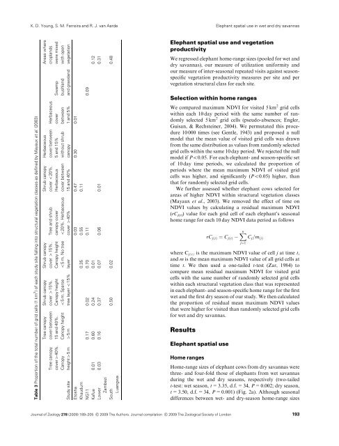
K. D. Young, S. M. Ferreira and R. J. van AardeElephant spatial use in wet and dry savannasTable 3 Proportion of the total number of grid cells (1 km 2 ) of each study site falling into structural vegetation classes as defined by Mayaux et al. (2003)Areas wherecroplandswere mixedwith openvegetationSwampbushlandand grasslandHerbaceouscoverbetween1 and 5%Herbaceouscover between5 and 15%without shrubcanopyShrub canopycover o20%.Herbaceouscover between15 and 40%Tree and shrubcanopy covero20%. Herbaceouscover 440%Shrub canopycover 415%.Canopy heighto5 m. No treelayerShrub canopycover 415%.Canopy heighto5 m. Sparsetree layer o15%Tree canopycover between15 and 40%.Canopy height45mTree canopycover440%.Canopyheight45mStudy siteEtosha 0.03 0.47 0.30 0.01Khaudum 0.35 0.55 0.11NG11 0.17 0.02 0.70 0.11 0.09Kafue 0.01 0.60 0.24 0.01 0.12Lower 0.03 0.16 0.37 0.07 0.06 0.01 0.31ZambeziSouthLuangwa0.50 0.02 0.48Elephant spatial use and vegetationproductivityWe regressed elephant home-range sizes (pooled for wet anddry savannas), our measure of utilization uniformity andour measure of inter-seasonal repeated visits against seasonspecificvegetation productivity measures per site and pervegetation structural class for each site.Selection within home rangesWe compared maximum NDVI for visited 5 km 2 grid cellswithin each 10 day period with the same number of randomlyselected 5 km 2 grid cells (pseudo-absences; Engler,Guisan, & Rechsteiner, 2004). We permutated this procedure10 000 times (see Gentle, 1943) and proposed a nullmodel that the mean value of visited grid cells was drawnfrom the same distribution as values from randomly selectedgrid cells within the same 10 day period. We rejected the nullmodel if Po0.05. For each elephant- and season-specific setof 10 day time periods, we calculated the proportion ofperiods where the mean maximum NDVI of visited gridcells was higher, and significantly (Po0.05) higher, thanthat for randomly selected grid cells.We further assessed whether elephant cows selected forareas of higher NDVI within structural vegetation classes(Mayaux et al., 2003). We removed the effect of time onNDVI values by calculating a residual maximum NDVI(rC j(t) ) value for each grid cell of each elephant’s seasonalhome range for each 10 day NDVI data period as followsrC jðtÞ ¼ C jðtÞX nj¼1C j =m ðtÞwhere C j(t) is the maximum NDVI value of cell j at time t,and m is the mean maximum NDVI value of all grid cells attime t. We then used a one-tailed t-test (Zar, 1984) tocompare mean residual maximum NDVI for visited gridcells with the same number of randomly selected grid cellswithin each structural vegetation class that was representedin each elephant- and season-specific home range for the firstwet and the first dry season of our study. We then calculatedthe proportion of residual mean maximum NDVI valuesthat were higher for visited than randomly selected grid cellsfor wet and dry savannas.ResultsElephant spatial useHome rangesHome-range sizes of elephant cows from dry savannas werethree- and four-fold those of elephants from wet savannasduring the wet and dry seasons, respectively (two-tailedt-test: wet season, t=3.35, d.f.=34, P=0.002; dry season,t=3.50, d.f.=34, P=0.001) (Fig. 2a). Although seasonaldifferences between wet- and dry-season home-range sizesJournal of Zoology 278 (2009) 189–205 c 2009 The Authors. Journal compilation c 2009 The Zoological Society of London 193
Page 1: Journal of ZoologyElephant spatial
Page 6: Elephant spatial use in wet and dry
Page 11 and 12: K. D. Young, S. M. Ferreira and R.
Page 17: K. D. Young, S. M. Ferreira and R.

Journal of Zoology - CERU - University of Pretoria

You also want an ePaper? Increase the reach of your titles

Delete template?

Save as template?