Did you know . . . - the National Drought Mitigation Center

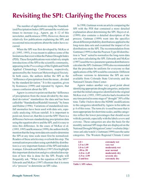
Revisiting the SPI: Clarifying the ProcessThe number of applications using the StandardizedPrecipitation Index (SPI) around the world continuesto increase (e.g., Agnew, pp. 6–12 of thisnewsletter, and Komuscu 1999). However, there arerelatively few publications explaining the SPI, andoccasional misconceptions about the index have occurred.When the SPI was first developed by McKee etal. (1993, 1995), it was meant to address some of thelimitations that exist within the Palmer Drought Index(PDI). These first publications were relatively simpleintroductions of the SPI to the scientific community,appearing in the Proceedings of the Eighth and NinthApplied Climatology Conferences, respectively,sponsored by the American Meteorological Society.In both cases, the authors define the SPI as the“difference of precipitation from the mean...dividedby the standard deviation.” It is this equation, givenby Komuscu (1999) and repeated by Agnew, thatcauses confusion about the SPI.Agnew is correct to point out that the “differenceof precipitation from the mean divided by the standarddeviation” standardizes the data and has beencalled the “Standardized Rainfall Anomaly” by Jonesand Hulme (1996). Variations of standardized rainfallanomalies have been used with data sets, especiallyanalyzing African rainfall. It is important topoint out, however, that this is not the SPI! There is adifference between standardizing precipitation datausing the equation above and the SPI, and it is easy tomiss this difference. In the cases of McKee et al.(1993, 1995) and Komuscu (1999), the authors brieflymention that the long-term data sets used to determinethe SPI at any time scale must first be normalized.Readers of these articles may overlook this step. Thenormalization procedure using a probability distributionis a very important feature of the SPI and makesit unique. Edwards and McKee (1997) first highlightthis important distinction and give a detailed descriptionof how this is done for the SPI. People willfrequently ask, “What is the equation of the SPI?”Edwards and McKee (1997) illustrate that it is moreof a “process” to determine an SPI value.In 1998, Guttman wrote an article comparing theSPI with the PDI that contained a more detailedexplanation about determining the SPI. Hayes et al.(1999) also contains a detailed description of theprocess. Guttman (1999) went into the specificsabout different probability distributions applied to thelong-term data sets and examined the impact of sixdistributions on the SPI. The recommendation fromGuttman (1999) is that the Pearson Type III distributionis “best” suited to normalize the long-term datasets when calculating the SPI. Edwards and McKee(1997) used the two-parameter gamma distribution tocalculate the SPI. Guttman (1999) also recommendedthat the procedure be uniform for everyone so thatapplications of the SPI would be consistent. Differentsoftware versions to determine the SPI are nowavailable from Colorado State University and theNational Climatic Data Center.Agnew makes another very good point aboutidentifying appropriate drought categories, and pointsout that the initial categories identified in the originalMcKee et al. (1993, 1995) articles had a location forany time period in some stage of “drought” 50% of thetime. Table 1 below shows the NDMC modificationsto the categories identified by Agnew in his table onp. 6 of this issue. The term dry is used because that ismore appropriate for short time scales, and the categoriesreflect the lower percentages that should occurwith dry periods, especially with the labels severe andextreme. These categories are also the basis for themonthly national SPI maps that are displayed on theNational Drought Mitigation Center’s website (http://enso.unl.edu/watch/). Guttman (1999) uses the samecategories. The Western Regional Climate Center2.0 + extremely wet1.5 to 1.99 very wet1.0 to 1.49 moderately wet-.99 to .99 near normal-1.0 to -1.49 moderately dry-1.5 to -1.99 severely dry-2 and less extremely dryTable 1. SPI values.Drought Network News13