Techniques in oscillatory shear rheology - Indian Institute of ...

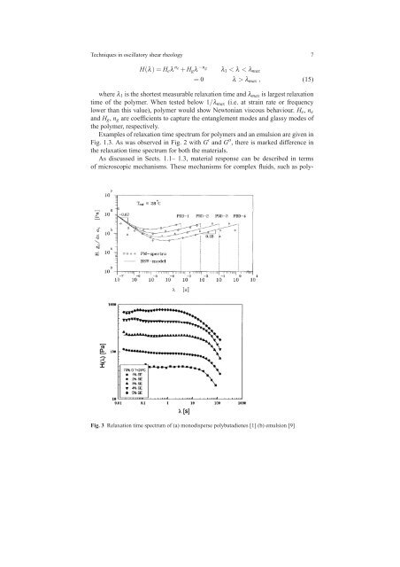
Techniques in oscillatory shear rheology 7H(λ) = H e λ n e+ H g λ −n gλ 1 < λ < λ max= 0 λ > λ max , (15)where λ 1 is the shortest measurable relaxation time and λ max is largest relaxationtime of the polymer. When tested below 1/λ max (i.e. at strain rate or frequencylower than this value), polymer would show Newtonian viscous behaviour. H e , n eand H g , n g are coefficients to capture the entanglement modes and glassy modes ofthe polymer, respectively.Examples of relaxation time spectrum for polymers and an emulsion are given inFig. 1.3. As was observed in Fig. 2 with G ′ and G ′′ , there is marked difference inthe relaxation time spectrum for both the materials.As discussed in Sects. 1.1– 1.3, material response can be described in termsof microscopic mechanisms. These mechanisms for complex fluids, such as poly-Fig. 3 Relaxation time spectrum of (a) monodisperse polybutadienes [1] (b) emulsion [9]