Vandermonde systems on Gauss-Lobatto Chebyshev nodes

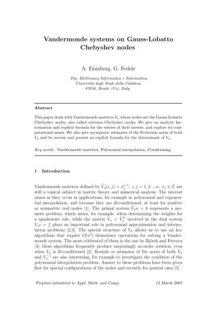
<strong>Vandermonde</strong> <strong>systems</strong> on Gauss-LobattoChebyshev nodesA. Eisinberg, G. FedeleDip. Elettronica Informatica e Sistemistica,Università degli Studi della Calabria,87036, Rende (Cs), ItalyAbstractThis paper deals with <strong>Vandermonde</strong> matrices V n whose nodes are the Gauss-LobattoChebyshev nodes, also called extrema Chebyshev nodes. We give an analytic factorizationand explicit formula for the entries of their inverse, and explore its computationalissues. We also give asymptotic estimates of the Frobenius norm of bothV n and its inverse and present an explicit formula for the determinant of V n .Key words: <strong>Vandermonde</strong> matrices, Polynomial interpolation, Conditioning1 Introduction<strong>Vandermonde</strong> matrices defined by Ṽn(i,j) = x i−1j , i,j = 1, 2...,n; x j ∈ C arestill a topical subject in matrix theory and numerical analysis. The interestarises as they occur in applications, for example in polynomial and exponentialinterpolation, and because they are ill-conditioned, at least for positiveor symmetric real nodes [1]. The primal system Ṽna = b represents a momentproblem, which arises, for example, when determining the weights fora quadrature rule, while the matrix V n = Ṽ nT involved in the dual systemV n c = f plays an important role in polynomial approximation and interpolationproblems [2,3]. The special structure of V n allows us to use ad hocalgorithms that require O(n 2 ) elementary operations for solving a <strong>Vandermonde</strong>system. The most celebrated of them is the one by Björck and Pereyra[4]; these algorithms frequently produce surprisingly accurate solution, evenwhen V n is ill-conditioned [2]. Bounds or estimates of the norm of both V nand Vn−1 are also interesting, for example to investigate the condition of thepolynomial interpolation problem. Answer to these problems have been givenfirst for special configurations of the nodes and recently for general ones [5].Preprint submitted to Appl. Math. and Comp. 12 March 2005

Polynomial interpolation on several set of nodes has received much attentionover the past decade [6]. Theoretically, any discretization grid can be used toconstruct the interpolation polynomial. However, the interpolated solution betweendiscretization points are accurate only if the individual building blocksbehave well between points. Lagrangian polynomials with a uniform grid sufferfor the effect of the Runge phenomenon: small data near the center of theinterval are associated with wild oscillations in the interpolant, on the order2 n times bigger, near the edges of the interval, [7][8]. The best choice is touse nodes that are clustered near the edges of the interval with an asymptoticdensity proportional to (1 − x 2 ) −1/2 as n → ∞, [9]. The family of Chebyshevpoints, obtained by projecting equally spaced points on the unit circle down tothe unit interval [−1, 1] have such density properties. The classical Chebyshevgrids are [10]:• Chebyshev nodesT 1 ={x k = cos• Extended Chebyshev nodes[ ]}2k − 12n π , k = 1, 2,...,n⎧⎨T 2 =⎩ x k = − cos ( ⎫2k−12n π)⎬cos ( ) , k = 1, 2,...,nπ⎭2n• Gauss-Lobatto Chebyshev nodes (extrema)T 3 ={x k = − cos[ ]}k − 1n − 1 π , k = 1, 2,...,n(1)(2)(3)In [11] it is proved that interpolation on the Chebyshev polynomial extremaminimizes the diameter of the set of the vectors of the coefficients of all possiblepolynomials interpolating the perturbed data. Although the set of Gauss-Lobatto Chebyshev nodes failed to be a good approximation to the optimalinterpolation set, such set is of considerable interest since the norm of correspondinginterpolation operator P n (T 3 ) is less than the norm of the operatorP n (T 1 ) induced by interpolation at the Chebyshev roots [12].This paper deals with <strong>Vandermonde</strong> matrices on Gauss-Lobatto Chebyshevnodes. Through the paper we present a factorization of the inverse of such matrixand derive an algorithm for solving primal and dual system. We also giveasymptotic estimates of the Frobenius norm of both V n and its inverse and anexplicit formula for det(V n ). A point of interest in this matrix is the (relative)moderate growth, versus n, of the condition number κ 2 (V n ), [13][3]. Figure 1shows the κ 2 comparison between the <strong>Vandermonde</strong> matrix on the Chebyshevnodes (V n (T 1 )), Chebyshev extesa nodes (V n (T 2 )) and Gauss-Lobatto Chebyshevnodes (V n (T 3 )).2

1κ 2(V n(T 3)/κ 2(V n(T 1))κ 2(V n(T 3)/κ 2(V n(T 2))0.950.90.850.80.750.70 10 20 30 40 50 60 70 80 90 100Fig. 1. Plot of the ratios κ 2(V n(T 3 ))κ 2 (V n(T 1 )) and κ 2(V n(T 3 ))κ 2 (V n(T 2 )) .n2 PreliminariesLet V n be the <strong>Vandermonde</strong> matrix defined on the set of n distinct nodesX n = {x 1 ,...,x n }:V n (i,j) = x j−1i , i,j = 1,...,n (4)In [14] the authors show that the inverse of the <strong>Vandermonde</strong> matrix V n ,namely W n , is:W n (i,j) = φ(n,j)ψ(n,i,j), i,j = 1,...,n (5)where the function ψ(n,i,j) is defined as:n−iψ(n,i,j) = (−1) i+j ∑(−1) r x r jσ(n,n − i − r), i,j = 1,...,n (6)r=0and the functions σ(m,s) and φ(m,s) are recursively defined as follows:3

⎧σ (m,s) = σ (m − 1,s) + x m σ (m − 1,s − 1) , m,s integer⎪⎨σ(m, 0) = 1, m = 0, 1,...(7)⎪⎩ (s < 0) ∨ (m < 0) ∨ (s > m) → σ (m,s) = 0⎧φ(m + 1,s) = φ(m,s)x m+1 −x s,m integer; s = 1,...,m⎪⎨∏φ(m + 1,m + 1) = m 1xk=1 m+1 −x k(8)⎪⎩ φ(2, 1) = φ(2, 2) = 1x 2 −x 1By (5), taking into account the (6), W n can be factorized as:where:W n = S · P · F (9)S(i,j) = (−1) i+j+1 σ(n,n + 1 − i − j), i = 1,...,n;j = 1,...,n + 1 − i(10)P(i,j) = (−1) j x i−1j , i,j = 1,...,n (11)F = diag {φ(n,i)} i=1,2,...,n(12)Note that:m∏m∑S m (x) = (x − x i ) = (−1) r σ (m,r) x m−r (13)i=1r=0S m(x ′ k ) = (−1) m+k 1, k = 1,...,m (14)φ(m,k)4

3 Main resultsWe start by noting that, for some sets of interpolation nodes, explicit expressionfor σ and φ may be found in [15]. We consider the set of Gauss-LobattoChebyshev nodes (X n = T 3 ) and give the proof of some properties useful inthe sequel.Lemma 1⎧σ(n, 2s) = (−1) s 1⌊∑n 2 ⌋ ( ) n−1 q2 ⎪⎨2q−1)( n−2 s , s = 0,..., ⌊n⌋ 2q=1(15)⎪⎩ σ(n, 2s + 1) = 0, s = 0,..., ⌈ n⌉ 2where notations ⌊·⌋ and ⌈·⌉ denote the floor and ceiling functions, respectively[16].Proof. It is easy to show that (13) can be rewritten as:whereS n (x) = 12 n−2(x − 1)(x + 1)U n−2(x) (16)U m (x) =sin [(m + 1) arccos(x)]sin [arccos(x)]is the m-order Chebyshev polynomial of the second kind.But [17]:⌊ n 2 ⌋ ( )∑ n − 1U n−2 (x) = (−1) q+1 x n−2q (1 − x 2 ) q−1 (17)2q − 1q=1by substituting the (17) in (16) one has:and, therefore, the (15) follows.⌊ n 2 ⌋ ( )∑ q∑ n − 1 qS n (x) = (−1) s xq=1 s=02q − 1)( n−2s (18)s5

Lemma 2S ′ n(x k ) = n − 12 n−2 [(−1) n+k − (−1) n δ k,1 + δ k,n](19)Proof. The (16) can be rewritten as:S n (x) = 1[(n + 1) arccos(x)]2n−2(x − 1)(x + 1)sinsin [arccos(x)]therefore, by standard algebraic manipulations:S ′ n(x k ) = 11 cos ( k−1n−12n−2(n − 1) cos [(n − k)π] − π)2 n−2 √ ( sin [(n − k)π]1 − cos 2 k−1n−1 π)Noting that:limk→1cos ( k−1n−1 π)√1 − cos 2 ( k−1n−1 π) sin [(n − k)π] = (−1) n (n − 1)limk→ncos ( k−1n−1 π)√1 − cos 2 ( k−1n−1 π) sin [(n − k)π] = −(n − 1)the (19) follows.By substituting the (19) in (14), one has:⎧⎪⎨φ(n,k) =⎪⎩2 n−3n−1k = 1,n2 n−2n−1k = 2,...,n − 1(20)Lemma 3 An alternative formulation of (15) is:σ(n, 2s) = (−1) s 1 ( ) n − s n 2 ⌊ ⌋− n − 2sn2 2s s (n − s − 1)(n − s) , s = 0, 1,..., 2(21)6

Proof. By the recurrence properties of the second-kind Chebyshev polynomials[18], one has:S n (x) − xS n−1 (x) + 1 4 S n−2(x) = 0therefore⌊ n 2 ⌋∑s=0σ(n, 2s)x n−2s −x⌊ n−12 ⌋∑s=0σ(n−1, 2s)x n−2s−1 + 1 4⌊ n−22 ⌋∑s=0σ(n−2, 2s)x n−2s−2 = 0(22)must holds. The (22) can be proved by standard algebraic manipulations whenn is both odd and even.By rearranging (10), (11) and (12), one has:⎧S(i,j) = (−1) i σ(n,n + 1 − i − j), i = 1,...,n;j = 1,...,n + 1 − i⎪⎨P(i,j) = cos [ j−1n−1 π] i−1, i,j = 1,...,n(23)⎪⎩ F(i,i) = (−1) i φ(n,i)i = 1,...,nFollowing the same line in [19], the matrix P can be factorized as:P = D · U · H (24)where:⎧⎪⎨D(i,i) = 12 i−2 , i = 2,...,n(25)⎪⎩ D(1, 1) = 17

⎧U(2i − 1, 1) = ( ) ⌈ ⌉2i−3i−1 , i = 1,..., n2⎪⎨U(2i, 2j) = ( ) ⌊ ⌊ ⌋2i−1i−j , j = 1,..., n2⌋, i = j,...,n2(26)⎪⎩U(2i − 1, 2j − 1) = ( ) ⌈ ⌈ ⌉2i−2i−j , j = 2,..., n2⌉, i = j,...,n2[ ](i − 1)(j − 1)H(i,j) = cos π , i = 1,...,n, j = 1,...,n (27)n − 1If one defines the matrix Q as:Q(i,j) = 2 n−i−1 [S · D · U] (i,j), i,j = 1,...,n (28)the (9) becomes:W n = 1n − 1 K · Q · H · F (29)whereK = diag{2 i−1 } i=1,2,...,n (30)⎧F(1, 1) = − 1 2⎪⎨F(i,i) = (−1) i , i = 2,...,n − 1(31)⎪⎩ F(n,n) = (−1) n 1 2We present here an efficient scheme for the computation Q. It can be shownthat Q can be build by the following equalities:8

⎧Q(1, n − 2) = 2Q(i, n + 1 − i) = (−1) ii = 1, 2, ..., n⎪⎨ Q(1, n − 2j − 2) = −Q(1, n − 2j),j = 1, 2, ..., ⌈ n−42 ⌉Q(i, n + 1 − i − 2j) = −Q(i, n + 3 − i − 2j) − Q(i − 1, n + 2 − i − 2j), i = 2, 3, ..., n;j = 1, 2, ..., j ∗⎪⎩ Q(i,1) = Q(i,1)/2,i = 1, 2, ..., n(32)where⎧⎪⎨j ∗ =⎪⎩⌊ n−i2 ⌋ n even⌈ n−1−i2⌉ n odd4 The Frobenius norm of V n and W nProposition 1 The Frobenius norm of V n is√ n − 1‖V n ‖ F = n +2 + √ 2 (n − 1) Γ ( n + )122n−3 π Γ(n)(33)where Γ(x) is the gamma function [20].Proof.‖V n ‖ 2 F =n∑n∑i=1 s=1[ ( )] s − 1 2i−2cosn − 1 π (34)But9

[ ( )] s − 1 2i−2cosn − 1 π =(1 2i − 22 2i−2 i − 1)+ 1 ∑i−2( 2i − 22 2i−2 2kk=0)cos[ 2(i − 1 − k)(s − 1)n − 1]π(35)then (34) becomes:‖V n ‖ 2 F =n∑n∑i=1 s=1 k=0n∑n∑i=1 s=1i−2 ∑)(1 2i − 22 2i−2 i − 1)22 2i−2 ( 2i − 2k+[ ]2(i − 1 − k)(s − 1)cosπn − 1(36)By using the identityn∑n∑i=1 s=1( )1 2i − 2= 22 2i−2 i − 1√ n Γ ( n + 1 2π Γ(n))(37)and by standard algebraic manipulations the (33) follows.Proposition 2 The Frobenius norm of W n is given by‖W n ‖ 2 F =[12(n − 1) + 22n−4β 1 (n) + 1 ]n − 1 n − 1 β 2(n)(38)whereβ 1 (n) =n∑k=1⌊ n−k∑2 ⌋ ⌊ n−k∑2 ⌋r=0s=0(−1) n+k+r+s (− 1 2n − k − r − s)σ(2r)σ(2s) (39)andβ 2 (n) =n∑k=1⌊ n−k2 ⌋∑r=0⌊ n−k2 ⌋ ∑s=01σ(2r)σ(2s) (40)2Proof. The (38) follows from standard algebraic manipulations.Taking into account only the term β 1 (n) in (38) and using the facts10

10 x 10−3 n98765432120 30 40 50 60 70 80 90 100Fig. 2. Relative error estimating ||W n || F .n∑k=1⌊ n−k∑2 ⌋ ⌊ n−k∑2 ⌋r=0q∑s=0s=0we give the following conjecture.Conjecture 1‖W n ‖ F∼ √ 2n − 1⌊ n 2 ⌋−1 ∑p=1[·] =⌊∑n−12 ⌋ ⌊∑n−12 ⌋ n−2max (r,s)∑r=0( ) p −32 q=s − 1)(s⌊ n 2 ⌋−1 ∑q=1( n − 12p − 1s=0k=1( ) p + q −32q − 1)( n − 12q − 1[·])( p + q −32q − 1), n → ∞(41)Figure 2 shows the accuracy of the estimate of the Frobenius norm of W n interm of relative error for n in the interval [20, 100] by Eq. 41.5 The determinant of V nThe next proposition gives the value of the determinant of V n .11

Proposition 3det(V n ) = 2√(n − 1)n2 n(n−2) (42)Proof. By the definition of the <strong>Vandermonde</strong> determinant we havedet(V n ) == 2 n(n−1)2∏1≤i

of both our and Björck-Pereyra algorithm. A set of experiments has been run,for n = 3 ÷ 10, 20, 30, 40, 50, 100. We have generated the right-hand sides fand b with random entries uniformly distributed in the interval [−1, 1]. Tables1 and 2 shows maximum and mean value of (43) and (44) over 10000 runs, thefraction of trials in which the proposed algorithms (EF) give equal or moreaccurate result than Björck-Pereyra ones (BP) and also the probability thatɛ c and ɛ a is less or equal than 10nu where u = 2 −53 is the unit roundoff. Asto the computational cost the EF algorithms require 3n 2 + O(n) while BPalgorithms cost 2.5n 2 + O(n) flops. EF algorithms seem to perform betterthan the Björck-Pereyra ones in terms of numerical accuracy and stability asit can be seen for high value of n. Same results are obtained by computingthe approximate solutions ĉ and â in Matlab package and then by migratingthe output in Mathematica in order to compare it with the “exact” one. ForMatlab code refer to Appendix A.n BP EF s.r.max mean max mean EF vs BP p(ɛ c ≤ 10nu)3 2.34-13 3.07-16 2.15-15 4.02-17 0.98 0.994 1.73-12 2.53-15 4.03-13 1.09-15 0.75 0.995 9.31-12 5.82-15 4.65-12 1.51-15 0.93 0.986 1.43-11 1.40-14 1.54-12 2.41-15 0.94 0.977 2.47-11 2.35-14 6.60-12 4.36-15 0.96 0.978 3.24-10 7.90-14 5.67-12 4.69-15 0.99 0.959 6.20-11 6.12-14 1.12-12 2.94-15 0.99 0.9610 1.56-10 1.98-13 9.00-12 6.66-15 0.99 0.9520 1.17-06 4.10-10 5.47-11 2.54-14 1.00 0.9230 2.10-03 9.79-07 2.22-09 3.86-13 1.00 0.9140 5.68+00 3.77-03 1.91-10 1.01-13 1.00 0.9250 7.61+03 1.38+01 4.04-11 9.49-14 1.00 0.90100 8.52+20 1.69+18 1.68-09 7.45-13 1.00 0.88Table 1. Dual problem. Maximum and mean value of ɛ c. Success rate of EF algorithm over 10000 runs.13

n BP EF s.r.max mean max mean EF vs BP p(ɛ a ≤ 10nu)3 1.70-13 2.90-16 5.46-13 3.26-16 0.79 0.994 1.06-10 1.33-14 3.25-11 3.99-15 0.74 0.985 3.96-11 8.87-15 7.94-13 1.32-15 0.86 0.976 6.69-11 2.68-14 3.68-12 2.57-15 0.91 0.977 2.93-11 1.66-14 4.69-12 2.91-15 0.95 0.978 6.00-11 3.52-14 2.48-12 3.15-15 0.98 0.969 9.70-11 4.33-14 6.00-12 3.16-15 0.96 0.9610 8.44-11 7.77-14 3.06-11 7.37-15 0.98 0.9520 1.12-08 3.25-12 4.49-11 1.98-14 1.00 0.9430 1.89-07 9.62-11 2.43-11 2.81-14 1.00 0.9340 1.22-05 4.26-09 2.13-10 4.33-14 1.00 0.9550 1.52-05 3.18-08 1.84-11 2.56-14 1.00 0.94100 3.88+02 1.68-01 1.71-10 7.30-14 1.00 0.94Table 2. Primal problem. Maximum and mean value of ɛ a. Success rate of EF algorithm over 10000 runs.7 ConclusionIn this paper we derived an explicit factorization of the <strong>Vandermonde</strong> matrixon Gauss-Lobatto Chebyshev nodes. Such factorization allows to design anefficient algorithm to solve <strong>Vandermonde</strong> <strong>systems</strong>. The numerical experimentsindicate that our approach is more stable compared with existing Björck-Pereyra algorithm. Starting from these theoretical results we are working witha conjecture on discrete orthogonal polynomials on Gauss-Lobatto Chebyshevnodes and its proof. The operation count and the accuracy obtained in theexperiments on least-squares problems seems to be very competitive.Appendix A - Matlab codefunction c=glc(f);n=max(size(f));nf=floor(n/2);f(1)=f(1)/2;14

f(n)=f(n)/2;for i=1:nf(i)=(-1)^i*f(i);end% Matrix H%--------------------------------------------------------H=zeros(n);H(1,1:nf)=ones(1,nf);H(1:nf,1)=ones(nf,1);if rem(n,2)==0start=1;elsefor j=1:ceil(n/2)H(nf+1,2*j-1)=(-1)^(j+1);endH(:,nf+1)=H(nf+1,:)’;start=2;endfor i=2:nffor j=i:nfH(i,j)=cos(rem((i-1)*(j-1),2*n-2)*pi/(n-1));H(j,i)=H(i,j);endendfor j=1:nfif rem(j,2)==0H(nf+start:n,j)=-flipud(H(1:nf,j));elseH(nf+start:n,j)=flipud(H(1:nf,j));endendfor i=1:nif rem(i,2)==0H(i,nf+start:n)=-fliplr(H(i,1:nf));elseH(i,nf+start:n)=fliplr(H(i,1:nf));endend%--------------------------------------------------------% Matrix Q%--------------------------------------------------------Q=zeros(n);for i=1:nQ(i,n+1-i)=(-1)^i;end15

Q(1,n-2)=2;for j=1:ceil((n-4)/2)Q(1,n-2*j-2)=-Q(1,n-2*j);endfor i=2:nif rem(i,2)==0jmax=floor((n-i)/2);elsejmax=ceil((n-1-i)/2);endfor j=1:jmaxQ(i,n+1-i-2*j)=-Q(i,n+3-i-2*j)-Q(i-1,n+2-i-2*j);endendQ(:,1)=Q(:,1)/2;%--------------------------------------------------------aux=H*f;c=zeros(n,1);for i=1:nfor j=rem(n+i,2)+1:2:n+1-ic(i)=c(i)+Q(i,j)*aux(j);endendfor i=1:nc(i)=2^(i-1)*c(i);endc=c/(n-1);References[1] Gautschi, W., Inglese, G., Lower bounds for the condition number of<strong>Vandermonde</strong> matrix, Numer. Math., 52 (1998), 241-250.[2] Golub, G. H., Van Loan, C. F., Matrix Computation, third ed., Johns HopkinsUniv. Press, Baltimore, MD, 1996.[3] Higham, N. J., Accuracy and Stability of Numerical Algorithms, SIAM,Philadelphia, PA, 1996.[4] Björck, A., Pereyra, V., Solution of <strong>Vandermonde</strong> <strong>systems</strong> of linear equations,Math. of Computation, 24 (1970), 893-903.[5] Tyrtyshnikov, E., How bad are Hankel matrices, Numer. Math., 67 (1994), 261-269.16

[6] Meijering, E., A Chronology of Interpolation: From Ancient Astronomy toModern Signal and Image Processing, Proc. of IEEE, 90 (2002), 319-342.[7] Björck, A., Dahlquist, G., Numerical Methods, Prentice-Hall, Englewood Cliffs,NJ, 1974.[8] Henrici, P., Essentials of Numerical Analysis, Wiley, New York, 1982.[9] Berrut, J. P., Trefethen, L. N., Barycentric Lagrange interpolation, SIAM Rev.46(2004), 501-517.[10] Brutman, L., Lebesgue functions for polynomial interpolation - a survey, Annalsof Numerical Mathematics, 4 (1997), 111-127.[11] Belforte, G., Gay, P., Monegato, G., Some new properties of Chebyshevpolynomials, J. Comput. Appl. Math., 117 (2000), 175-181.[12] Brutman, L., A note on polynomial interpolation at the Chebyshev extremanodes, Journal of Approx. Theory, 42 (1984), 283-292.[13] Gautschi, W., Norms estimates for inverses of <strong>Vandermonde</strong> matrices, Numer.Math., 23 (1974), 337-347.[14] Eisinberg, A., Picardi, C., On the inversion of <strong>Vandermonde</strong> matrix, Proc. ofthe 8th Triennial IFAC World Congress, Kyoto, Japan, 1981.[15] Eisinberg, A., Fedele, G., Polynomial interpolation and related algorithms,Twelfth International Colloquium on Num. Anal. and Computer Science withAppl., Plovdiv, 2003.[16] Knuth, D. E., The Art of Computer Programming, vol. 1, second ed., Addison-Wesley, Reading, MA, 1973.[17] Gradshteyn, I. S., Ryzhik, I. M., Table of Integrals, Series and Products, thirded., Academic Press, New York, 1965.[18] Rivlin, T. J., The Chebyshev Polynomials, John Wiley & Sons, New York, 1974.[19] Eisinberg, A., Franzé, G., Salerno, N., Rectangular <strong>Vandermonde</strong> matrices onChebyshev nodes, Linear Algebra Appl., 338 (2001), 27-36.[20] Gatteschi, L., Funzioni Speciali, UTET, 1973.[21] Wolfram, S., Mathematica: a System for Doing Mathematics by Computers,Second. ed., Addison-Wesley, 1991.17