Introductory Econometrics Exercises for tutorials

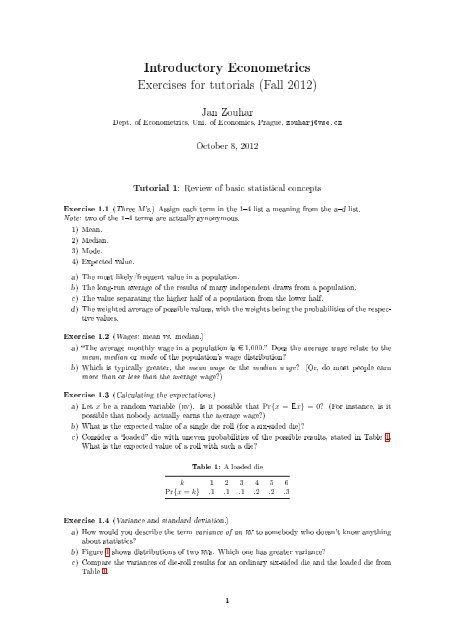
Introductory econometrics: exercises for tutorialsJan ZouharFigure 1: Two distributions, dierent variancesd) Assume that height of a person is approximately normally distributed with a mean of 180 cmand variance σ 2 . What percentage of the population falls within ±σ from the populationaverage (i.e., in the interval [180 − σ, 180 + σ])? And how about the ±2σ or ±3σ range? Drawa plot that illustrates this.e) rv x has the following characteristics: Ex = 10, varx = 0. Is there anything more we can sayabout x?Exercise 1.5 (Calculations with expected value and variance.) Let x and y be independent rvswithEx = 10, Ey = 5,varx = 1, var y = 2.Calculate:a) E[4x].b) E[4x + 5].c ) E[x + y].d) E[x − y].e) E[4x − 3y + 5].f ) var[4x].g ) var[4x + 5].h) var[x + y].i) var[x − y].j) var[4x − 3y + 5].Exercise 1.6 (Multiple dice.)a) Imagine we roll two six-sided dice and add up the results. What are the possible outcomes?What are their probabilities? Draw a plot of the probability function.b) What is the variance of the rv from a? (Hint: the variance of a die roll is 3512 .)c ) Suppose we take the arithmetic average of 10 die rolls. What is the expected value and varianceof the result?Exercise 1.7 (Random sample and sample mean.) The population distribution of the number ofteeth (x) has a mean of 20 with a variance of 100. Assume we draw (at random) a sample of 10people, measure the value of x for each one of them (thus obtaining values x 1 , x 2 , . . . , x 10 ), and thencalculate the arithmetic average ¯x = 1 ∑ 1010 i=1 x i. Due to random sampling, ¯x is a random variable.a) What is the expected value of ¯x? What is its variance?b) (Law of large numbers.) Instead of 10 people, we take n now. What happens to E ¯x and var ¯xif we gradually raise n above all limits?c ) (Central limit theorem.) Again, consider a sample of n people, only that now we study theresult ofy = √ ∑ ni=1n(¯x − 20) =(x i − 20)√ . nAs n grows, what happens to the distribution of y?Exercise 1.8 (Visualizing the central limit theorem.) Download the CLT.zip archive from mywebsite and run the CLT.m le in Matlab. You should obtain a gure similar to Figure 2. It showsprobability distributions of standardized means (see below) of samples with dierent sizes, drawnfrom the population stored in vector x in the Matlab code, line 4. Here, a standardized mean is the2

Introductory econometrics: exercises for tutorialsJan Zouharexpression √ n(¯x − µ), where µ is the population average. Therefore, the gure shows the eect ofthe central limit theorem (clt). The starting population is {1,2,3,4,5,6}, which means that eachobservation is in fact a die roll. Notice how fast the distributions converge to the bell-shaped curveof normal (or Gaussian) distribution. Try changing the population, perhaps repeating some of thenumbers, and see how the convergence process changes.Figure 2: Die-roll standardized means (clt demonstration)Exercise 1.9 (Correlation & covariance.)a) Would you say that wages and education are positively correlated, negatively correlated oruncorrelated? And how about wages a person's height?b) Find an example of negatively correlated economic variables.c ) If we know that two rvs are negatively correlated, what does it tell us about their covariance?d) What are the possible values of a covariance of two rvs?e) Let x and y be independent. Is it possible that cov(x, y) = 0.58? Why?f ) We know that cov(x, y) = 0. Do x and y have to be independent? (If not, nd an example ofrvs that are uncorrelated despite not being independent.)g ) What are the possible values of a correlation coecient of two rvs?h) Which of the following can happen:1) corr(x, y) = −1.56.2) corr(x, y) = 0.28, cov(x, y) = 0.3) corr(x, y) = 0.28, cov(x, y) = −0.5.4) corr(x, y) = 0.28, cov(x, y) = 0.5.Why? What is the relationship between the covariance and correlation coecient of two rvs?Exercise 1.10 (Sharpening your eyes.) In your web browser, type in the addresshttp://www.ruf.rice.edu/~lane/stat_sim/reg_by_eye/.Follow the instructions on the website: rst press the begin button in the upper-left corner, thenlook at the scatterplot of two rvs (we'll denote them x and y here), and guess which of the vesuggested numbers for corr(x, y) is correct. To see the correct value, click on the Show r button.Repeat the procedure (using the New Data button) until you manage to guess the right answer threetimes in a row.Exercise 1.11 (Conditional expectations.)3

Introductory econometrics: exercises for tutorialsJan Zouhara) What is the average monthly wage in your country, expressed in e? (Make a rough guess.)b) Imagine you meet a person on the street and he/she tells you he/she had only nished elementaryschool before getting employed. Does this information change your expectation about theperson's wage?c ) Estimate the following: E[wage|educ = 9], E[wage|educ = 13], E[wage|educ = 18]. 1d) Based on c, try to approximate E[wage|educ] using a linear relationshipE[wage|educ] = β 0 + β 1 educ.e) Based on d, what is the expected dierence in wages for two people with a gap of 1 yearin their education? In other words, what is the population average of ∆wage? (Or: what is∆E[wage|educ]∆educ?)Exercise 1.12 (Calculations with conditional expectations.)∆educa) Let x and y be independent rvs, Ey = 12.5. Find E[y|x].b) Let x and y be rvs, E[y|x] = 2 + 5x. Find E[4y + 3xy + x 2 |x] and E[4y + 3xy + x 2 |x = 5].Exercise 1.13 (Conditional expectations II.) Suppose that at a large university, college grade pointaverage, GPA, and SAT score, SAT , are related by the conditional expectationE[GPA|SAT ] = .70 + .002 SAT .a) Find the expected GPA when SAT = 800. Find E[GPA|SAT = 1,400]. Comment on thedierence.b) If the average SAT in the university is 1,100, what is the average GPA?Exercise 1.14 (Conditional variance.) Do you think the variance of wages varies among groups ofpeople with dierent levels of education? E.g., is there a dierence between var[wage|educ = 9] andvar[wage|educ = 18]?Tutorial 2: Simple regressionExercise 2.1 (Gretl practice.) Import data from the MS Excel le simplereg.xls into Gretl (usethe drag-and-drop trick). (This is a ctitious dataset, the numbers don't have any real meaning.)a) Regress y on x; i.e., estimate (using Model → Ordinary least squares) the modelE[y|x] = β 0 + β 1 x.b) Write down the estimated regression function. (Note: once we've estimated a model, wetypically write ŷ = ˆβ 0 + ˆβ 1 x.)c ) From the Gretl output, read the value of R 2 . What does it tell us about the model?d) Find (in Gretl or by calculation) the values of SST, SSR and SSE.e) Draw the scatterplot of x i 's and y i 's with the estimated regression line in it (Graphs → Fitted,actual plot → Against x).f ) Save the residuals (û i ) from the estimated model as a new variable (Save → Residuals). Next,nd the sample mean of û (View → Summary Statistics) and sample correlation between ûand x (View → Correlation Matrix). Is the result unexpected, or can we generalize it to otherregression models? Explain why.Exercise 2.2 (Campaign expenditures.) Load the data voting.gdt. The data describe electionoutcomes and campaign expenditures for 173 two-party races (A,B) for the U.S. House of Representativesin 1988.1 Here educ is expressed in years, i.e. 9 years typically represent elementary education and 18 years a master's degree.4

Introductory econometrics: exercises for tutorialsJan Zouhara) Consider the following regression model:E[voteA|expenA] = β 0 + β 1 expenA.Does it make sense to use a model like this to describe the relationship between campaignexpenditures and the eventual vote share? How would you interpret β 0 and β 1 ? In a twopartyrace, do you think it makes sense to look at the campaign expenditures of party Aalone?b) Consider the following regression model:E[voteA|shareA] = β 0 + β 1 shareAwhere shareA is A's percentage share in the total campaign expenditures (total meaning thesum across all parties). Generate shareA in Gretl (use Add → Dene new variable), estimatethe model and interpret the estimates.c ) Find a story for the association between voteA and shareA supporting each of the three causationschemes.Exercise 2.3 (Constant elasticity model.) Load the data ceosal1.gdt (the ceos' salaries datafrom Lecture 2). This time, we relate salary to sales.a) Consider the following population regression model:log(salary) = β 0 + β 1 log(sales) + u.Can you express the elasticity of salary with respect to sales in terms of the regression coecientsβ 0 and β 1 ?b) Generate log(salary) and log(sales) in Gretl (use Add → Logs of selected variables) and estimatethe regression model.c ) Regress salary on sales without logarithms and look at the R 2 's in both models. Does acomparison of the two R 2 's tell us something meaningful?Exercise 2.4 (Monte Carlo.) In the lectures, we study the linear regression model (lrm) usinganalytical means. There's another way to study the linear regression model, and that is using acomputer simulation. Consider a population modely = β 0 + β 1 x + u, β 0 = 5, β 1 = 10 (1)and a random sample consisting of 15 observations. Carry out the following simulation in MS Excel.You can use the MonteCarlo.xls le if you like.a) Generate x and u values at random and write them down in two columns. Use the RAND-BETWEEN function to do this (the function generates a random integer within the speciedbounds). You can pick any range for x; however, note that in a clrm, Eu has to be zero.Therefore, the lower and upper bounds for u have to be opposite numbers; i.e., use RANDBE-TWEEN(−u max , u max ).b) Create columns with both y and E[y|x]; these will be calculated based on (1).c ) Draw a scatterplot of y vs. x and include the prf in it (i.e., the line E[y|x] = β 0 + β 1 x). PressF9 repeatedly to see how the random sampling procedure looks like. What does u representin the plot?d) Calculate the ols-estimates ˆβ 0 and ˆβ 1 using INTERCEPT and SLOPE functions. Next, calculatethe values of ŷ and û, and add the srf line (i.e., the line ŷ = ˆβ 0 + ˆβ 1 x) into your plot. Press F9repeatedly to see how accurately the ols procedure estimates β 0 and β 1 . Which one is moreaccurate (on average), ˆβ 0 or ˆβ 1 ?e) Press F9 ten times, write down the results for ˆβ 0 and ˆβ 1 , and then make the arithmetic averageof the 10 trials for both ˆβ 0 and ˆβ 1 . What results would you expect if we did 1000 trials insteadof 10?5

Introductory econometrics: exercises for tutorialsJan Zouharf ) Open the MonteCarlo2.xls le. The experiment from e is automated here, only with 1000trials instead of 10. The 1000 values of ˆβ 0 and ˆβ 1 are shown in columns W and AC. In the samecolumns, you can see the mean and (sample) standard deviation of the 1000 trials. Comparethe standard deviations for ˆβ 0 and ˆβ 1 . Does the dierence in the two values reect yourconclusions about the accuracy of the estimates?g ) The histogram plots on the right show the frequencies of ˆβ0 (green) and ˆβ 1 (blue) valuesamong the 1000 trials in the experiment. These plots tell us something about the shape of thedistribution of rvs ˆβ 0 and ˆβ 1 . Does the shape of the plots remind you of one of the well-knowndistributions?Exercise 2.5 (Conditional variance of ˆβ1 using Monte Carlo simulation.) In the lectures, wederived a formula for conditional variance of ˆβ 1 given x by analytical means. In this exercise, you'llverify the result using Monte Carlo simulation. In principle, this will be the same simulation as inthe previous exercise, only that now we study the conditional distribution of ˆβ 1 . In order to do this,we need to select particular values of the explanatory variable and keep these values xed in therepeated samples (i.e., only the values of u are sampled each time, x remains the same). Proceedas follows:a) Open the MonteCarlo3.xls le.b) Select specic values for x; e.g., replace the formulas in the green column I with odd numbersgoing from 1 to 29.c ) Look at the sample variance of the resulting 1000 trials for ˆβ 1 in cell X1006. Compare thisnumber to the analytic result, which saysvar[ ˆβ 1 |x] = σ2s 2 .xNote that s 2 x = ∑ 15i=1 (x i − ¯x) 2 and σ 2 is the variance of u. We're using RANDBETWEEN togenerate u, which means u has discrete uniform distribution, the variance of which is(b − a − 1) 2 − 1,12where a and b are the lower and upper bound, respectively. (Fill the formulas for σ 2 , s 2 xand var[ ˆβ 1 |x] in cells Q5, Q6 and Q7, respectively.) Press F9 repeatedly and comment on thedierence between the analytical and simulation results.Exercise 2.6 (Factors aecting ˆβ 1 variance.) We'll continue working with the MonteCarlo3.xlsle. From the lectures, you know that . . .i) . . . the less variance in the disturbances,ii) . . . the more variance in the explanatory variable,the more accurate estimates we obtain. Verify this using the simulation model.a) Try changing the range of x-values (e.g., pick the numbers 1024 or 070) and see how thevariance of the estimates varies.b) Try changing the u max value and watch the resulting change in the variance of the estimates.Tutorial 3: Multiple regression IExercise 3.1 (Sleep vs. work). The following model is a simplied version of the multiple regressionmodel used by Biddle and Hamermesh (1990) to study the tradeo between time spent sleeping andworking and to look at other factors aecting sleep:sleep = β 0 + β 1 totwrk + β 2 educ + β 3 age + u,where sleep and totwrk (total work) are measured in minutes per week and educ and age aremeasured in years.6

Introductory econometrics: exercises for tutorialsJan Zouhara) If adults trade o sleep for work, what is the sign of β 1 ?b) What signs do you think β 2 and β 3 will have?c ) Using the data in sleep.gdt, estimate the model and write out the results in equation form.d) If someone works ve more hours per week, by how many minutes is sleep predicted to fall?Is this a large tradeo?e) Discuss the sign and magnitude of the estimated coecient on educ.f ) Would you say totwrk, educ, and age explain much of the variation in sleep? What otherfactors might aect the time spent sleeping? Are these likely to be correlated with totwrk?Exercise 3.2 (Housing prices and pollution). The following equation describes the median housingprice in a community in terms of amount of pollution (nox for nitrous oxide) and the average numberof rooms in houses in the community (rooms):log(price) = β 0 + β 1 log(nox) + β 2 rooms + u. (2)a) What are the probable signs of β 1 and β 2 ? What is the interpretation of β 1 ? Explain.b) Why might nox (or the log of nox ) and rooms be negatively correlated? If this is the case,does the simple regression of log(price) on log(nox) produce an upward or downward biasedestimator of β 1 ?c ) Using the data in houses.gdt, estimate (2) and the following model:log(price) = β 0 + β 1 log(nox) + u.Is the relationship between the simple and multiple regression estimates of the elasticity ofprice with respect to nox what you would have predicted, given your answer in part b? Doesthis mean that ˆβ 1 from (2) is denitely closer to the true elasticity than ˆβ 1 from the simpleregression model?Exercise 3.3 (Building up an econometric model). You were asked to carry out empirical researchin order to quantify the so-called returns to schooling, i.e., the eect of additional education on aperson's wage. In lecture 1, we discussed the steps to be carried out in empirical analysis:Step 1:Step 2:Step 3:Step 4:Step 5:Step 6:Formulate the question of interest.Find a suitable economic model.Turn it into an econometric model.Obtain suitable data.Use econometric methods to estimate the econometric model.If needed, use hypothesis tests to answer the question of interest.Step 1 has already been made for you: the question of interest is stated above. Your task here is todiscuss steps 2, 3 and 4 in detail.a) Put up a list of all thinkable factors that shape a person's wage.b) Try to argue the causal link from each of the factors to a person's wage from the standpointof an economic theory. Arguments such as we all know that clever people earn more moneydo not count here.c ) Explain how you would quantify the factors you identied. First, decide whether a factor isdirectly measurable, or whether we need to nd a suitable proxy variable. Second, explainwhat units you'd use use for quantication.d) Write down the econometric model you would use in order to estimate the eect of wages oneducation. Is it necessary to include all the factors (or their proxies) in the regression model?Are some of them more important than others?e) Is it possible to drop one of the variables you included in the model without violating theE[u|educ] = 0 assumption?f ) Based on your economic argumentation from b, what values of the β parameters do you expect?(For each jth variable, give at least the expected sign of β j .)7

Introductory econometrics: exercises for tutorialsJan Zouharg ) Imagine you've collected the data you need and saved them into an MS Excel le. Sketch astructure of the MS Excel le (think up arbitrary data for the rst two observations).Tutorial 4: Multiple regression IIExercise 4.1 (Partialling out). Using the 526 observations on workers in wage.gdt, regress the logof wage (hourly wage in $) on educ (years of education), exper (years of labor market experience),and tenure (years with the current employer).a) Formulate the population regression model you are estimating.b) Write down the estimated equation and interpret the values of the estimated coecients.c ) Conrm the partialling out interpretation of the ols estimates by explicitly doing the partiallingout. This rst requires regressing educ on exper and tenure, and saving the residuals,ˆr 1 . Then, regress log(wage) on ˆr 1 . Compare the coecient on ˆr 1 with the coecient on educin the regression from b.Exercise 4.2 (Working with categories). In a study relating college grade point average to timespent in various activities, you distribute a survey to several students. The students are asked howmany hours they spend each week in four activities: studying, sleeping, working, and leisure. Anyactivity is put into one of the four categories, so that for each student the sum of hours in the fouractivities must be 168.a) Consider the modelGPA = β 0 + β 1 study + β 2 work + β 3 leisure + β 4 sleep + u.Interpret the coecient β 1 . Does it make sense to hold work, leisure, and sleep xed, whilechanging study?b) Explain why this model violates Assumption MLR.3.c ) How could you reformulate the model so that its parameters have a useful interpretation andit satises Assumption MLR.3?Exercise 4.3 (Harmless multicollinearity ). Suppose you postulate a model explaining nal examscore in terms of class attendance. Thus, the dependent variable is nal exam score, and the keyexplanatory variable is number of classes attended. To control for student abilities and eortsoutside the classroom, you include among the explanatory variables cumulative GPA, SAT score,and measures of high school performance. Someone says, You cannot hope to learn anything fromthis exercise because cumulative GPA, SAT score, and high school performance are likely to behighly collinear. What should be your response?Exercise 4.4 (Variable selection). The causal links between variables y, x, z 1 , z 2 , z 3 and z 4 areshown in Figure 3. Your task is to quantify the causal eect of x on y. Which of the variables willyou include in your equation?y z 1 z 2 z 3z 4xFigure 3: Causal links between variables y, x, z 1, z 2, z 3 and z 4Exercise 4.5 (Used cars). The le used_cars_original.xls contains data on used ’kodas thatI collected in January 2004. At that time, I owned an old ’koda Felicia and was thinking aboutselling it; I didn't sell it in the end, and later in 2009, it suddenly caught re when my dad wasdriving it (accidentaly, this happened very close to our university premises), see8

Introductory econometrics: exercises for tutorialsJan Zouharhttp://www.pozary.cz/clanek/20375-obrazem-u-bulhara-horela-skodovka/.When you open the le in MS Excel, you'll notice that the data format is not suitable for econometricwork (why?). Compare used_cars_original.xls with used_cars.xls and notice the way thequalitative variables were encoded into dummies.a) Regress price on km and age; interpret all the estimated coecients. Is there any meaningfulinterpretation of the intercept? Do you nd its level reasonable?b) Regress price on km and year now. Compare the results with your previous model. Howwould you interpret the intercept in this case?c ) In the data, I created the variable age from the year of manufacture in the following way:age = 2004 − year. Notice the impact this relationship had on the coecients you estimatedin a and b.d) Regress price on all available explanatory variables. Why were some of the variables omittedby Gretl? Interpret the coecients for the dummy variables that were retained.e) Try and nd the best regression model for the price of a used ’koda. Consider (and estimate)various function forms.f ) How much value does a used car lose (on average) with each additional kilometre? Discuss thevarious function shapes you used in e.g ) What price would you ask (in 2004) for ’koda Felicia, which has 100.000 km on the clock, theengine 1.9D and was manufactured in 1998?h) Would be a version with petrol engine be cheaper? By how much?i) What is the price dierence between used Octavias and Felicias? What data will you use tond this out?j) Find out whether the extra charge for the combi version varies for Octavias and Felicias.k ) Find out whether the extra charge for a diesel engine varies for Octavias and Felicias.l) Find out whether the average value loss per km varies for Octavias and Felicias.Tutorial 5: Hypothesis testingExercise 5.1 (Theory check). Which of the following can cause the usual ols t statistics to beinvalid (that is, not to have t distributions under H 0 )?a) Heteroskedasticity.b) A sample correlation coecient of .95 between two independent variables that are in the model.c ) Omitting an important explanatory variable.Exercise 5.2 (Practical vs. statistical signicance). Consider an equation to explain salaries ofceos in terms of annual rm sales, return on equity (roe, in percent form), and return on the rm'sstock (ros, in percent form):log(salary) = β 0 + β 1 log(sales) + β 2 roe + β 3 ros + u.a) In terms of the model parameters, state the null hypothesis that, after controlling for sales androe, ros has no eect on ceo salary. State the alternative that better stock market performanceincreases a ceo's salary.b) Esitmate the equation using the data in ceosal1.gdt. By what percent is salary predicted toincrease, if ros increases by 50 points? Does ros have a practically large eect on salary?c ) Test the null hypothesis that ros has no eect on salary, against the alternative that ros hasa positive eect. Carry out the test at the 10% signicance level.d) Would you include ros in a nal model explaining ceo compensation in terms of rm performance?Explain.Exercise 5.3 (Individual vs. joint signicance). Using the data in sleep.gdt, estimateand report the results in equation form.sleep = β 0 + β 1 totwrk + β 2 educ + β 3 age + u9

Introductory econometrics: exercises for tutorialsJan Zouhara) Is either educ or age individually signicant at the 5% level against a two-sided alternative?Show your work.b) Drop educ and age from the equation and report the results in equation form. Are educ andage jointly signicant in the original equation at the 5% level? Justify your answer.c ) Does including educ and age in the model greatly aect the estimated tradeo between sleepingand working?d) Suppose that the sleep equation contains heteroskedasticity. What does this mean about thetests computed in parts a and b?Exercise 5.4 (Using condence intervals to test hypotheses). The variables in GPA.gdt includecollege grade point average (colGPA), high school GPA (hsGPA), achievement test score (ACT ),and the average number of lectures missed per week (skipped) for a sample of 141 students from alarge university; both college and high school GPAs are on a four-point scale. Estimate the followingequation, which can be used to study the eects of skipping class on college GPA:colGPA = β 0 + β 1 hsGPA + β 2 ACT + β 3 skipped + u.a) Using the standard normal approximation, nd the 95% condence interval for hsGPA.b) Can you reject the hypothesis H 0 : hsGPA = .4 against the two-sided alternative at the 5%level?c ) Can you reject the hypothesis H 0 : hsGPA = 1 against the two-sided alternative at the 5%level?Exercise 5.5 (Linear restrictions). Use the data in wages2.gdt for this exercise.a) Consider the standard wage equationlog(wage) = β 0 + β 1 educ + β 2 exper + β 3 tenure + u.State the null hypothesis that another year of general workforce experience has the same eecton log(wage) as another year of tenure with the current employer.b) Test the null hypothesis in part a against a two-sided alternative, at the 5% signicance level,by constructing a 95% condence interval. What do you conclude?10