Dynamic modal characteristics of transverse vibrations of cantilevers ...

402 D.I. Caruntu / Mechanics Research Communications 36 (2009) 391–404
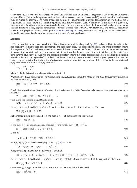
can be used (1) as a source of basic design for situations which happen to fall within the geometry and boundary conditions
presented here, (2) for studying forced and nonlinear vibrations of these cantilevers, and (3) as test cases for the development
of numerical methods. The mode shapes can be used (4) as admissible functions for approximate methods as well.
In general exact mode shapes and natural frequencies have the advantage of being of great ease for further use. In particular,
hypergeometric functions, which are exact mode shapes in this work, are versatile tools. They are included as special mathematical
functions in very popular commercial software packages such as MAPLE, MATHEMATICA, and MATLAB. Also, their
mathematical properties are well developed Abramovitz and Stegun (1965). The results of this paper are limited to Euler-
Bernoulli cantilevers, i.e. they are not accurate in the case of short cantilevers.
Appendix
This shows that the necessary condition of finite displacement at the sharp end, Eq. (27), is also a sufficient condition for
free boundary, leading to zero bending moment and zero shear force. Two propositions follow. The first proposition shows
that in general if a function is continuous on an interval closed at one end, so finite at this end, and its derivatives are continuous
on the open interval, then these are sufficient conditions for the existence of the limits at this end of certain functions
involving function’s derivatives. The second proposition shows that using proposition one zero bending moment and
zero shear force at a sharp end of a parabolic cantilever result. Lagrange’s theorem is used to prove proposition one. Lagrange’s
theorem states that if a function y(x) is continuous in a closed interval [a,b], and differentiable in the open interval
(a,b), then there is a c value in (a,b) such that
y 0 yðbÞ
ðcÞ ¼
b
yðaÞ
;
a
ð54Þ
where 0 =dy/dx. Without loss of generality consider b =1.
Proposition 1. Given a function y(x), continuous on an interval closed at one end (a,1] and its first three derivatives continuous on
the open interval (a,1) then
limð1
xÞ
x!1 n y ðnÞ ðxÞ ¼0; n ¼ 1; 2; 3: ð55Þ
Proof. Due to continuity of function y(x)atx =1,y(1) exists and it is finite. According to Lagrange’s theorem there is a c value
such that
yð1Þ yðxÞ ¼y 0 ðcÞð1 xÞ; x < c < 1: ð56Þ
Thus, using the triangle inequality, it results
jyð1Þ yðxÞj ¼ jy 0 ðcÞð1 xÞj P jy 0 ðcÞð1 cÞj P 0: ð57Þ
If x ? 1, then c ? 1, and jy(1 ) y(x)j ? 0 due to continuity at x = 1 of the function y(x). Therefore
0 P lim jy
c!1
0 ðcÞð1 cÞj P 0 ð58Þ
and consequently, using x instead of c, the case of n = 1 of the proposition is obtained
limð1
xÞy
x!1 0 ðxÞ ¼0: ð59Þ
In the case of n = 2, using Lagrange’s theorem for the function g(x)=(1 x)y 0 (x).
It results
gð1Þ gðxÞ ¼g 0 ðcÞð1 xÞ; x < c < 1: ð60Þ
y 0 ðxÞ ¼ð1 cÞy 00 ðcÞ y 0 ðcÞ; x < c < 1: ð61Þ
Multiplying by (1 c) and rearranging terms, Eq. (61) becomes
ð1 cÞy 0 ðxÞþð1 cÞy 0 ðcÞ ¼ð1 cÞ 2 y 00 ðcÞ: ð62Þ
Using the triangle inequality the following is obtained:
jð1 xÞy 0 ðxÞj þ jð1 cÞy 0 ðcÞj P j ð1 cÞy 0 ðxÞþð1 cÞy 0 ðcÞj ¼ jð1 cÞ 2 y 00 ðcÞj P 0: ð63Þ
If x ? 1, then c ? 1, and both j(1 x)y 0 (x)j ? 0 and j(1 c)y 0 (c)j ? 0 due to case n = 1 of the proposition. Therefore
0 P lim jð1
c!1
cÞ 2 y 00 ðcÞj P 0: ð64Þ
Consequently, using x instead of c, the case of n = 2 of the proposition is obtained
limð1
xÞ
x!1 2 y 00 ðxÞ ¼0: ð65Þ