Dynamic modal characteristics of transverse vibrations of cantilevers ...

Dynamic modal characteristics of transverse vibrations of cantilevers 

of parabolic thickness 

Dumitru I. Caruntu * 

University of Texas-Pan American, Mechanical Engineering Department, Edinburg, TX 78541, USA 

article info 

Article history: 

Received 2 January 2008 

Received in revised form 12 May 2008 

Available online 30 July 2008 

Keywords: 

Nonuniform cantilevers 

Parabolic thickness 

Exact natural frequencies 

Exact mode shapes 

1. Introduction 

abstract 

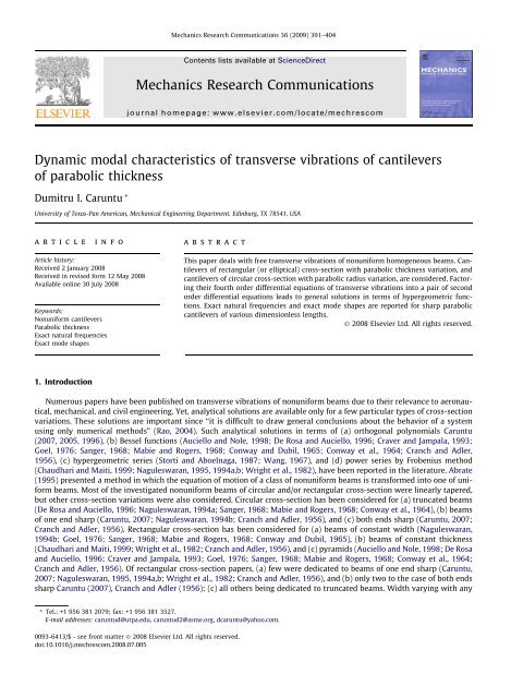
This paper deals with free transverse vibrations of nonuniform homogeneous beams. Cantilevers 

of rectangular (or elliptical) cross-section with parabolic thickness variation, and 

cantilevers of circular cross-section with parabolic radius variation, are considered. Factoring 

their fourth order differential equations of transverse vibrations into a pair of second 

order differential equations leads to general solutions in terms of hypergeometric functions. 

Exact natural frequencies and exact mode shapes are reported for sharp parabolic 

cantilevers of various dimensionless lengths. 

Ó 2008 Elsevier Ltd. All rights reserved. 

Numerous papers have been published on transverse vibrations of nonuniform beams due to their relevance to aeronautical, 

mechanical, and civil engineering. Yet, analytical solutions are available only for a few particular types of cross-section 

variations. These solutions are important since ‘‘it is difficult to draw general conclusions about the behavior of a system 

using only numerical methods” (Rao, 2004). Such analytical solutions in terms of (a) orthogonal polynomials Caruntu 

(2007, 2005, 1996), (b) Bessel functions (Auciello and Nole, 1998; De Rosa and Auciello, 1996; Craver and Jampala, 1993; 

Goel, 1976; Sanger, 1968; Mabie and Rogers, 1968; Conway and Dubil, 1965; Conway et al., 1964; Cranch and Adler, 

1956), (c) hypergeometric series (Storti and Aboelnaga, 1987; Wang, 1967), and (d) power series by Frobenius method 

(Chaudhari and Maiti, 1999; Naguleswaran, 1995, 1994a,b; Wright et al., 1982), have been reported in the literature. Abrate 

(1995) presented a method in which the equation of motion of a class of nonuniform beams is transformed into one of uniform 

beams. Most of the investigated nonuniform beams of circular and/or rectangular cross-section were linearly tapered, 

but other cross-section variations were also considered. Circular cross-section has been considered for (a) truncated beams 

(De Rosa and Auciello, 1996; Naguleswaran, 1994a; Sanger, 1968; Mabie and Rogers, 1968; Conway et al., 1964), (b) beams 

of one end sharp (Caruntu, 2007; Naguleswaran, 1994b; Cranch and Adler, 1956), and (c) both ends sharp (Caruntu, 2007; 

Cranch and Adler, 1956). Rectangular cross-section has been considered for (a) beams of constant width (Naguleswaran, 

1994b; Goel, 1976; Sanger, 1968; Mabie and Rogers, 1968; Conway and Dubil, 1965), (b) beams of constant thickness 

(Chaudhari and Maiti, 1999; Wright et al., 1982; Cranch and Adler, 1956), and (c) pyramids (Auciello and Nole, 1998; De Rosa 

and Auciello, 1996; Craver and Jampala, 1993; Goel, 1976; Sanger, 1968; Mabie and Rogers, 1968; Conway et al., 1964; 

Cranch and Adler, 1956). Of rectangular cross-section papers, (a) few were dedicated to beams of one end sharp (Caruntu, 

2007; Naguleswaran, 1995, 1994a,b; Wright et al., 1982; Cranch and Adler, 1956), and (b) only two to the case of both ends 

sharp Caruntu (2007), Cranch and Adler (1956); (c) all others being dedicated to truncated beams. Width varying with any 

* Tel.: +1 956 381 2079; fax: +1 956 381 3527. 

E-mail addresses: caruntud@utpa.edu, caruntud2@asme.org, dcaruntu@yahoo.com. 

0093-6413/$ - see front matter Ó 2008 Elsevier Ltd. All rights reserved. 

doi:10.1016/j.mechrescom.2008.07.005 

Mechanics Research Communications 36 (2009) 391–404 

Contents lists available at ScienceDirect 

Mechanics Research Communications 

journal homepage: www.elsevier.com/locate/mechrescom

392 D.I. Caruntu / Mechanics Research Communications 36 (2009) 391–404 

positive power of the longitudinal coordinate has been considered along with (a) constant thickness (Naguleswaran, 1995), 

(b) linear thickness (Sanger, 1968; Cranch and Adler, 1956), and (c) any positive power variation of thickness (Wang, 1967). 

Beams of parabolic thickness variation with particular boundary conditions and solutions in terms of orthogonal polynomials 

have been reported as well (Caruntu, 2007, 1996). Beams of exponential thickness and constant width were presented by 

Ece et al. (2007), and constant thickness and exponential width by Cranch and Adler (1956). An asymptotic approach for 

transverse vibrations of variable section beams has been reported by Firouz-Abadi et al. (2007). A recent mathematical investigation, 

Anderson and Hoffacker (2006), was dedicated to the existence of solutions of cantilever beam problem. As one can 

see there is a continuous effort in studying one dimensional continuous systems. 

Cantilevers of parabolic thickness variation are important for studies regarding geometry influence on different phenomena. 

Cantilevers in general are key structures in many engineering applications. In particular they are extensively used as 

resonator sensors. Cantilever structures are integral parts of microelectromechanical (MEMS) biosensors for the detection 

of airborne virus particles (Johnson et al., 2006), and resonant nanoelectromechanical systems (NEMS) for a new class of ultra 

fast, highly sensitive devices (Cimalla et al., 2007). Results regarding nonuniform cantilevers of particular geometry used 

as resonator sensors have been already reported in the literature. For instance Turner and Wiehn (2001) considered the 

dynamics of atomic force microscope (AFM) cantilevers in terms of flexural vibrations. They investigated the sensitivity of 

a nonuniform cantilever beam (triangular with constant width) against a uniform cantilever, and found that for values of 

a studied parameter (the normal contact stiffness relative to the stiffness of the cantilever) greater than 100, the overall sensitivity 

of the triangular cantilever is greater than or equal to that of the uniform beam. The fact that nonuniform cantilevers 

can be, under specific circumstances, more sensitive than uniform cantilevers is an important result. 

To the author’s best knowledge, there are virtually no dynamic modal characteristics available in the literature for transverse 

vibrations of cantilevers of parabolic thickness. This paper aims to fill this gap by presenting the general solution of the 

differential equation of transverse vibrations of parabolic cantilevers, and the exact natural frequencies and exact mode 

shapes for the boundary value problems of sharp parabolic cantilevers. This paper presents a different approach and consequently 

different results than those reported by Caruntu (2007) who reported the class of beams and plates whose boundary 

value problems can be reduced to an eigenvalue singular problem of orthogonal polynomials. In the work of Caruntu (2007) 

the natural frequencies and the mode shapes (which were Jacobi polynomials) resulted directly, without any frequency 

equation to be solved, from the eigenfunctions and eigenvalues of orthogonal polynomials reported by Caruntu (2005). In 

this work, the fourth order differential equation of motion is factored into a pair of second order differential equations. General 

solution in terms of hypergeometric functions, and frequency equation resulting from cantilever boundary conditions, 

are reported. The exact natural frequencies and exact mode shapes are found for sharp parabolic cantilevers by solving the 

frequency equation. 

This paper falls in the category of analytical methods and modeling for linear vibration, benchmark solutions. Results reported 

in this paper, along with already reported data for cantilevers linearly tapered (Cranch and Adler, 1956) and uniform 

cantilevers (Timoshenko et al., 1974) provide the necessary information for studies on geometry influences on free, forced, 

linear and/or nonlinear vibrations of such cantilevers. In particular the results of this paper are useful for studies on mass 

deposition sensitivity of resonator sensors. 

2. Transverse vibration of nonuniform Euler–Bernoulli beams 

Euler–Bernoulli differential equation of transverse vibrations of nonuniform beams is given by 

d 2 

dx2 EI ðxÞ d2yðxÞ dx2 " # 

q0x2 A ðxÞyðxÞ ¼0; x1 < x

The reference cross-section area and moment of inertia, A 0 and I 0, are considered at the longitudinal coordinate n = 0 (or 

x = 0), Fig. 1. 

3. Beam of rectangular cross-section and parabolic thickness 

3.1. Differential equation 

Consider a beam of rectangular cross-section, constant width w * (x), and parabolic thickness h * (x), Fig. 1, as follows: 

x 2 

w ðxÞ ¼w0 ¼ constant; h ðxÞ ¼h0 1 

‘ 2 ; x1 < x


3.2. General solution 

Eq. (10) can be factored as follows: 

ð1 n 2 Þ d2 

dn 2 4n d 

" # 

þ k1 

dn 

ð1 n 2 Þ d2 

dn 2 4n d 

" # 

þ k2 

dn 

Y ¼ 0; ð11Þ 

where 

kj ¼ 2 þð 1Þ j 

ffiffiffiffiffiffiffiffiffiffiffiffiffiffiffi 

4 þ x2 p 

; j ¼ 1; 2: ð12Þ 

Due to the factorization, solving the fourth order differential equation (10) reduces to solving the two second order differential 

equations which are given by Eq. (11). Using the variable changing 

n ¼ 1 2z; ð13Þ 

the two second order differential equations given by Eq. (11) become 

zð1 zÞ d2Y dY 

þ½2 4zŠ 

dz2 dz þ kjY ¼ 0; j ¼ 1; 2: ð14Þ 

Differential equations (14) are Gauss equations. As the canonical form of Gauss equation is 

zð1 zÞ d2y dy 

þ½c ðaþ b þ 1ÞzŠ 

dz2 dz 

abz ¼ 0; ð15Þ 

the Gauss coefficients, aj, bj, cj of the two differential equations (14) are given by 

8 

>< 

cj ¼ 2 

aj þ bj ¼ 3 

; j ¼ 1; 2: ð16Þ 

>: 

p 

ajbj ¼ 2 þð 1Þ j ffiffiffiffiffiffiffiffiffiffiffiffiffiffiffi 

4 þ x 2 

According to Abramovitz and Stegun (1965) the general solutions of the differential equations (14) are 

YjðzÞ ¼Aj 2F1ðaj; bj; cj; zÞþBj wj2ðzÞ; j ¼ 1; 2; ð17Þ 

where Aj, Bj, j = 1,2, are constants of integration, 2F1 (a,b,c,z) is the hypergeometric function 

2F1ða; b; c; zÞ ¼ X1 

n¼0 

wj2(z) function is given by 

ðaÞ n ðbÞ n 

ðcÞ n 

wj2ðzÞ ¼2F1ðaj; bi; cj; zÞ ln z þ X1 

zn ; ð18Þ 

n! 

n¼1 

þ wðcjÞ wðn þ 1Þþwð1ÞŠ Xc j 1 

ðajÞnðbjÞ n z 

n!ðcjÞn n ½wðaj þ nÞ wðajÞþwðbj þ nÞ wðbjÞ wðn þ cjÞ 

n¼1 

ðn 1Þ!ð1 cjÞn z 

ð1 ajÞnð1 bjÞn n ; ð19Þ 

wis the logarithmic derivative of Gamma function C, and (a)n is the Pochhammer symbol or rising factorial 

ðaÞ n ¼ 

Cða þ nÞ 

¼ aða þ 1Þ ...ða þ n 1Þ: ð20Þ 

CðaÞ 

Since the second order differential operators of Eq. (11) are commuting operators, the general solution Y(n) of Eq. (10) is a 

linear combination of the solutions Y1(n) and Y2(n), given by Eq. (17), as follows: 

YðnÞ ¼ X2 

j¼1 

1 n 

Aj 2F1 aj; bj; cj; 

2 

þ Bj wj2 

1 n 

2 

: ð21Þ 

The general solution given Eq. (21) holds for any beam of rectangular cross-section, constant width, and parabolic thickness 

variation, sharp or not, and any boundary conditions. Yet, only the case of sharp parabolic cantilevers is considered in 

what follows. Numerical determinations of the natural frequencies and mode shapes are presented in this case. 

3.3. Boundary conditions and frequency equation of sharp parabolic cantilevers 

Consider a parabolic cantilever with one end sharp. In this case both coefficients B 1 and B 2 of the general solution given by 

Eq. (21) must be zero, therefore the general solution in this case becomes

1 n 

YðnÞ ¼A1 2F1 a1; b1; c1; 

2 

1 n 

þ A2 2F1 a2; b2; c2; 

2 

: ð22Þ 

Both coefficients B 1 and B 2 must be zero because the functions w j2[(1 n)/2], j = 1,2, given by Eq. (19), become infinite at the 

sharp end, n = 1, due to the logarithmic function, and consequently the functions wj2, j = 1,2, cannot be used since the transverse 

displacement of the cantilever must always remain finite. On the boundary n = n 1, the fixed end of the cantilever, the 

following conditions have to be met: 

Yðn 1Þ¼ dY 

dn ðn 1Þ¼0: ð23Þ 

Therefore the boundary value problem in the case of sharp cantilevers is given by Eqs. (22) and (23), and it leads to the following 

natural frequency equation: 

Fðx2 Þ¼ 2F1ða1; b1; c1; 1 n1 2 Þ 2F1 a2; b2; c2; 1 n1 2 

a1b1 2F1 a1 þ 1; b1 þ 1; c1 þ 1; 1 n1 a2b2 2 2F1 a2 þ 1; b2 þ 1; c2 þ 1; 1 n1 2 

¼ 0; ð24Þ 

where coefficients aj, bj, cj, j = 1,2 are given by Eq. (16). Solving Eq. (24), the dimensionless natural frequencies xk are obtained. 

Denoting a jk ¼ ajðx kÞ; b jk ¼ bjðx kÞ; j ¼ 1; 2, the corresponding mode shapes Yk(n) result as 

1 n 

YkðnÞ ¼2F1 a1k; b1k; c1; 

2 

where the coefficients D k are given by 

Dk ¼ 2F1 a1k; b1k; c1; 1 n1 2 

2F1 a2k; b2k; c2; 1 n 1 

2 

1 n 

þ Dk 2F1 a2k; b2k; c2; 

2 

; ð25Þ 

: ð26Þ 

Few remarks regarding boundary conditions follow. First, if the free end of the cantilever was not sharp, i.e. it was a regular 

point of the differential equation, then the general solution of the equation of motion would be given by Eq. (21) and the free 

boundary conditions at this end would be those of zero bending moment and zero shear force. Second, at any sharp end, 

physically no specific displacement or slope can be enforced, so any sharp end must be a free end. Therefore no boundary 

such as pinned, fixed, or simply supported can occur at sharp ends. On the other hand, tacitly it is always required that 

the displacement and its derivatives are finite at every point of the cantilever. However, at the sharp end of the cantilever, 

n = 1, which is a singular point of the differential equation, the condition that the displacement is finite has to be explicitly 

enforced 

Yð1Þ ¼finite: ð27Þ 

Eq. (27) was the boundary condition that reduced Eq. (21) to Eq. (22). Third, the necessary condition of finite displacement 

at the sharp end, Eq. (27), Caruntu (2007), is a sufficient condition for zero bending moment and zero shear force (free 

boundary) in the case of parabolic sharp cantilever, see Appendix. This is consistent with the fact that a sharp end cannot 

sustain any moment or shear force. One can say that the usual boundary conditions of a free end, M = T = 0, zero bending 

moment and zero shear force, have to be replaced by Y = finite at a sharp end. Fourth, the finite displacement condition, 

Eq. (27), eliminates from the general solution given by Eq. (21) the unbounded at n = 1 functions w j2, j = 1,2, and leaves 

the general solution with only hypergeometric functions which are continuous and have continuous derivatives at n =1. 

3.4. Numerical determinations of exact modes 

The exact natural modes, reported in what follows, are of sharp parabolic cantilevers of rectangular (or elliptical) crosssection. 

Eq. (24) has been solved using MATLAB (and MATHEMATICA) to find the first four natural frequencies for different 

values of the dimensionless coordinate of the fixed end, n 1 = 1+k/10, where k =3,4,...,17. One can see from Fig. 1 that the 

cantilever dimensionless length is given by 1 n1. Table 1 shows the first four natural frequencies of the beam and Fig. 2 

graphs the first three natural frequencies. All the necessary coefficients for the corresponding mode shapes are given in Tables 

2 and 3. The Gauss coefficients given by Eq. (16) are found in Table 2, and D coefficients given by Eq. (26) are found in 

Table 1 

First four natural frequencies x ¼ x‘ 2 

n 1 

D.I. Caruntu / Mechanics Research Communications 36 (2009) 391–404 395 

pffiffiffiffiffiffiffiffiffiffiffiffiffiffiffiffiffiffiffiffiffiffiffiffiffiffiffi 

ðq0A0Þ=ðEI0Þ of the cantilever given in Fig. 1 versus the dimensionless coordinate of the fixed end n1 0.7 0.6 0.5 0.4 0.3 0.2 0.1 0 0.1 0.2 0.3 0.4 0.5 0.6 0.7 

x1 1.050 1.469 1.936 2.465 3.070 3.770 4.593 5.576 6.772 8.263 10.17 12.72 16.27 21.60 30.47 

x 2 7.606 8.958 10.42 12.02 13.83 15.91 18.32 21.18 24.65 28.96 34.47 41.78 51.99 67.26 92.66 

x 3 18.25 20.91 23.79 26.96 30.54 34.63 39.40 45.05 51.90 60.41 71.29 85.72 105.9 136.0 186.2 

x4 32.54 36.96 41.73 46.99 52.92 59.70 67.61 76.98 88.34 102.4 120.5 144.4 177.8 227.8 310.9


Dimensionless natural frequency 

200 

180 

160 

140 

120 

100 

Table 3. For instance one can read for the case of n 1 = 0 that the second dimensionless natural frequency is x2 ¼ 21:18 from 

Table 1, the Gauss coefficients for the corresponding mode shape given by Eq. (25) are a12 = 6.552 and a22 = 1.5 + 4.126i from 

Table 2, and D 2 = 17.78 10 4 from Table 3. The coefficients b 12 = 3.552 and b 22 = 1.5 4.126i result from Eq. (16). Therefore, 

for the case of n1 = 0, the second dimensionless natural frequency and mode shapes are 

x2 ¼ 21:18; ð28Þ 

1 n 

Y2ðnÞ ¼2F1 6:552; 3:552; 2; 

2 

80 

60 

40 

20 

0 

-0.8 -0.6 -0.4 -0.2 0 0.2 0.4 0.6 0.8 

Dimensionless coordinate of the fixed end 

Fig. 2. First three dimensionless natural frequencies x ¼ x‘ 2pffiffiffiffiffiffiffiffiffiffiffiffiffiffiffiffiffiffiffiffiffiffiffiffiffiffiffi 

ðq0A0Þ=ðEI0Þ of the cantilever, Fig. 1, versus the coordinate n1 of the fixed end; (––––) first 

frequency, (----) second frequency, and (......) third frequency. 

Table 2 

Gauss coefficients a 1k, a 2k of the first four mode shapes k = 1,2,3,4 (see Eq. (25)) of the cantilever given in Fig. 1 

a11 a21 a12 a22 a13 a23 a14 a24 n1 0.7 4.051 2.911 4.981 1.5 + 1.901i 6.255 1.5 + 3.756i 7.571 1.5 + 5.325i 

0.6 4.095 2.830 5.164 1.5 + 2.220i 6.526 1.5 + 4.094i 7.924 1.5 + 5.724i 

0.5 4.152 2.711 5.354 1.5 + 2.521i 6.803 1.5 + 4.430i 8.284 1.5 + 6.126i 

0.4 4.225 2.537 5.554 1.5 + 2.818i 7.094 1.5 + 4.774i 8.661 1.5 + 6.541i 

0.3 4.313 2.266 5.769 1.5 + 3.119i 7.404 1.5 + 5.134i 9.064 1.5 + 6.979i 

0.2 4.419 1.5 + 0.1329i 6.003 1.5 + 3.432i 7.740 1.5 + 5.517i 9.499 1.5 + 7.449i 

0.1 4.543 1.5 + 0.8715i 6.262 1.5 + 3.765i 8.110 1.5 + 5.933i 9.979 1.5 + 7.962i 

0 4.690 1.5 + 1.294i 6.552 1.5 + 4.126i 8.525 1.5 + 6.391i 10.51 1.5 + 8.530i 

0.1 4.863 1.5 + 1.677i 6.884 1.5 + 4.526i 8.996 1.5 + 6.906i 11.12 1.5 + 9.172i 

0.2 5.071 1.5 + 2.062i 7.269 1.5 + 4.978i 9.543 1.5 + 7.496i 11.83 1.5 + 9.910i 

0.3 5.324 1.5 + 2.474i 7.727 1.5 + 5.502i 10.19 1.5 + 8.190i 12.67 1.5 + 10.78i 

0.4 5.638 1.5 + 2.937i 8.288 1.5 + 6.130i 10.99 1.5 + 9.028i 13.69 1.5 + 11.84i 

0.5 6.044 1.5 + 3.485i 9.002 1.5 + 6.912i 11.99 1.5 + 10.08i 14.99 1.5 + 13.17i 

0.6 6.594 1.5 + 4.177i 9.958 1.5 + 7.940i 13.34 1.5 + 11.48i 16.73 1.5 + 14.95i 

0.7 7.398 1.5 + 5.127i 11.35 1.5 + 9.404i 15.30 1.5 + 13.49i 19.25 1.5 + 17.51i 

Table 3 

Coefficients D k of the first four mode shapes k = 1,2,3,4 (see Eq. (26)) of the cantilever given in Fig. 1 

D1 10 2 

D2 10 4 

D3 10 6 

D4 10 7 

n 1 

0.7 0.6 0.5 0.4 0.3 0.2 0.1 0 0.1 0.2 0.3 0.4 0.5 0.6 0.7 

45.25 33.83 25.41 19.30 14.86 11.62 9.219 7.424 6.060 5.009 4.187 3.537 3.016 2.593 2.247 

75.11 55.87 43.51 34.99 28.82 24.19 20.61 17.78 15.50 13.64 12.09 10.79 9.695 8.754 7.943 

152.7 125.6 106.0 91.18 79.61 70.32 62.73 56.40 51.06 46.50 42.57 39.15 36.16 33.51 31.16 

43.79 37.78 33.20 29.58 26.63 24.19 22.12 20.35 18.82 17.49 16.31 15.26 14.33 13.48 12.72 

17:78 10 4 

1 n 

2F1 1:5 þ 4:126i; 1:5 4:126i; 2; 

2 

: ð29Þ

Figure 3 shows the first three cantilever mode shapes for three different values of the dimensionless coordinates of the 

fixed end. One can use Fig. 1 to see the three geometry cases of the cantilever. 

3.5. Approximate natural frequencies by Galerkin method 

An approximate method, namely Galerkin method, is used to find approximations of the first two natural frequencies of 

transverse vibrations of a parabolic sharp cantilever whose fixed end is at n1 =0,Fig. 1, for comparison with the exact solutions 

reported in this paper. These approximations are shown to be close to the exact values reported in previous Section 3.4. 

The boundary value problem to be solved by Galerkin method is given by Eqs. (10) and (23). Look for a trial solution for the 

boundary value problem as follows 

yðnÞ ¼ X2 

i¼1 

biu i ðnÞ; ð30Þ 

where ui(n)=n i+1 , and bi are adjustable constants, i = 1,2. One can see that the trial solution satisfies the boundary conditions 

given by Eq. (23) and is finite at n =1.IfyðnÞ was the true solution, then it would satisfy Eq. (10) identically. An approximate 

solution by Galerkin method is found from the requirement that the differential operator of Eq. (10) be orthogonal to the 

linear span of {u i} which results into the following equations: 

Z 1 

0 

0.8 

0.6 

0.4 

0.2 

- 0.4 - 0.2 0.2 0.4 0.6 0.8 1.0 

- 0.2 


a 1.0 

b 

( ) 

uiðnÞ ð1 n 2 Þ 2 d 4 y 

dn 4 12nð1 n 2 Þ d3y dn 3 6ð1 5n 2 Þ d2y dn 2 

c 

1.0 

0.8 

0.6 

0.4 

0.2 

- 0.4 - 0.2 0.2 0.4 0.6 0.8 1.0 

- 0.2 

- 0.4 - 0.2 0.2 0.4 0.6 0.8 1.0 

- 0.2 

Fig. 3. First thee mode shapes of the cantilever given in Fig. 1 for three values of the dimensionless coordinate of the fixed end n 1: (a) n 1 = 0.4, (b) n 1 = 0.0, 

and (c) n 1 = 0.4. 

x2 y 

dn ¼ 0; i ¼ 1; 2; ð31Þ 

The constants bi are determined from Eq. (31). After calculations the following algebraic system is obtained: 

b1 8:0 x2 5 þ b2 15:0 x2 6 ¼ 0; 

b1 7:0 x2 6 þ b2 14:4 x2 8 

>< 

>: 

7 ¼ 0: 

This system of equations has nontrivial solutions if and only if its determinant is zero, which represents the eigenvalue 

equation. Solving this equation, the approximate values of the first two natural frequencies are found to be 5.54 and 20.44. 

These values are close to the exact values of 5.576 and 21.18 given in Table 1. 

1.0 

0.8 

0.6 

0.4 

0.2 

ð32Þ


4. Beams of circular cross-section and parabolic radius variation 

4.1. Differential equation 

Consider a beam of circular cross-section of parabolic radius variation, Fig. 4. The current radius R * (x) is given by 

x 2 

R ðxÞ ¼R0 1 

‘ 2 ; x1 < x

" # 

ð1 n 2 Þ d2 

dn 2 

6n d 

þ k1 

dn 

" # 

ð1 n 2 Þ d2 

dn 2 

6n d 

þ k2 

dn 

Y ¼ 0; ð39Þ 

where 

kj ¼ 3 þð 1Þ j 

ffiffiffiffiffiffiffiffiffiffiffiffiffiffiffi 

9 þ x2 p 

; j ¼ 1; 2: ð40Þ 

Using the variable changing given by Eq. (13), the two second order differential equations of the factored equation (39) become 

Gauss differential equations with coefficients aj, bj, cj given by 

8 

>< 

cj ¼ 3 

aj þ bj ¼ 5 

; j ¼ 1; 2: ð41Þ 

>: 

p 

ajbj ¼ 3 þð 1Þ j ffiffiffiffiffiffiffiffiffiffiffiffiffiffiffi 

9 þ x 2 

The general solution given by Eqs. (21) and (41) holds for any boundary conditions of parabolic cantilevers of circular 

cross-section. Eqs. (22) and (24) are the general solution and the frequency equation, respectively, of the boundary value 

problem of sharp parabolic cantilevers given by Eqs. (38) and (23), where the coefficients aj, bj, cj are given by Eq. (41). 

The mode shapes are given by Eqs. (25) and (41). Yet, only sharp parabolic cantilever case is considered for numerical 

determinations. 

4.3. Numerical determinations of exact modes 

The exact natural modes, reported in what follows, are of sharp parabolic cantilevers of circular cross-section. Eq. (24) 

with Gauss coefficients given by Eq. (41) has been solved using MATLAB (and MATHEMATICA) for finding the first four natural 

frequencies. Different values of the dimensionless coordinate of the fixed end, n1 = 1+k/10, where k =3,4,...,17, were 

considered. Table 4 shows the first four natural frequencies of the beam. Fig. 5 graphs the first three natural frequencies. All 

the necessary coefficients for the first four corresponding mode shapes are given in Tables 5 and 6. The Gauss coefficients are 

given in Table 5, and the D coefficients given by Eq. (26) are found in Table 6. For instance one can read for the case of n 1 =0 

Table 4 

First four natural frequencies x ¼ x‘ 2 

n 1 


ðq0A0Þ=ðEI0Þ of the cantilever given in Fig. 4 versus the dimensionless coordinate of the fixed end n1 0.7 0.6 0.5 0.4 0.3 0.2 0.1 0 0.1 0.2 0.3 0.4 0.5 0.6 0.7 

x1 1.011 1.572 2.238 3.020 3.940 5.026 6.322 7.886 9.805 12.21 15.31 19.45 25.26 33.97 48.49 

x 2 8.727 10.57 12.55 14.75 17.23 20.07 23.40 27.35 32.15 38.12 45.75 55.90 70.07 91.29 126.6 

x 3 21.25 24.49 28.12 32.14 36.68 41.88 47.96 55.18 63.93 74.80 88.71 107.2 133.0 171.6 235.8 

x 4 37.25 42.54 48.29 54.66 61.84 70.07 79.68 91.09 104.9 122.1 144.0 173.2 213.9 274.8 376.2 

Dimensionless natural frequency 

250 

200 

150 

100 

50 


0 

-0.8 -0.6 -0.4 -0.2 0 0.2 0.4 0.6 0.8 

Dimensionless coordinate of the fixed end 

Fig. 5. First three dimensionless natural frequencies x ¼ x‘ 2 


ðq0A0Þ=ðEI0Þ of the cantilever, Fig. 4, versus the coordinate n1 of the fixed end; (–––) first 

frequency, (----) second frequency, (...dots) third frequency.


Table 5 

Gauss coefficients a 1k, a 2k of the first four mode shapes k = 1,2,3,4 (see Eq. (25)) of the cantilever given in Fig. 4 

n1 a11 a21 a12 a22 a13 a23 a14 a24 0.7 6.024 4.967 6.799 2.649 8.033 2.5 + 3.480i 9.328 2.5 + 5.303i 

0.6 6.055 4.921 6.998 2.5 + 1.317i 8.324 2.5 + 3.927i 9.704 2.5 + 5.780i 

0.5 6.105 4.847 7.207 2.5 + 1.912i 8.626 2.5 + 4.362i 10.09 2.5 + 6.256i 

0.4 6.175 4.735 7.429 2.5 + 2.408i 8.944 2.5 + 4.799i 10.50 2.5 + 6.744i 

0.3 6.269 4.573 7.671 2.5 + 2.870i 9.286 2.5 + 5.249i 10.94 2.5 + 7.257i 

0.2 6.386 4.343 7.936 2.5 + 3.324i 9.658 2.5 + 5.722i 11.41 2.5 + 7.803i 

0.1 6.531 4.001 8.231 2.5 + 3.787i 10.07 2.5 + 6.229i 11.93 2.5 + 8.396i 

0 6.706 3.402 8.564 2.5 + 4.274i 10.53 2.5 + 6.783i 12.52 2.5 + 9.049i 

0.1 6.916 2.5 + 1.002i 8.945 2.5 + 4.800i 11.06 2.5 + 7.400i 13.19 2.5 + 9.783i 

0.2 7.172 2.5 + 1.824i 9.391 2.5 + 5.384i 11.67 2.5 + 8.100i 13.96 2.5 + 10.62i 

0.3 7.485 2.5 + 2.521i 9.923 2.5 + 6.050i 12.40 2.5 + 8.9173i 14.88 2.5 + 11.61i 

0.4 7.879 2.5 + 3.230i 10.58 2.5 + 6.836i 13.29 2.5 + 9.899i 16.01 2.5 + 12.81i 

0.5 8.389 2.5 + 4.023i 11.41 2.5 + 7.803i 14.43 2.5 + 11.12i 17.44 2.5 + 14.31i 

0.6 9.084 2.5 + 4.985i 12.53 2.5 + 9.060i 15.95 2.5 + 12.74i 19.36 2.5 + 16.30i 

0.7 10.11 2.5 + 6.272i 14.16 2.5 + 10.83i 18.15 2.5 + 15.05i 22.13 2.5 + 19.16i 

Table 6 

Coefficients D k of the first four mode shapes k = 1,2,3,4 (see Eq. (26)) of the cantilever given in Fig. 4 

D1 D2 D3 D4 10 2 

10 4 

10 6 

10 7 

n 1 

0.7 0.6 0.5 0.4 0.3 0.2 0.1 0 0.1 0.2 0.3 0.4 0.5 0.6 0.7 

50.88 37.14 26.45 18.64 13.17 9.397 6.809 5.019 3.765 2.871 2.224 1.748 1.392 1.122 0.914 

81.11 52.72 36.40 26.25 19.57 14.98 11.72 9.332 7.549 6.188 5.132 4.300 3.637 3.101 2.663 

113.6 86.18 67.02 53.26 43.10 35.42 29.50 24.86 21.16 18.17 15.73 13.71 12.03 10.62 9.417 

26.07 21.19 17.46 14.59 12.35 10.57 9.128 7.953 6.981 6.170 5.485 4.903 4.403 3.973 3.599 

that the second dimensionless natural frequency is x2 ¼ 27:35, and the coefficients for the corresponding mode shape given 

by Eq. (25) are a 12 = 8.564 and a 22 = 2.5 + 4.274i from Table 2, and D 2 = 9.332 10 4 from Table 3. The coefficients 

b12 = 3.564 and b22 = 2.5 4.274i result from Eq. (41). Therefore, for the case of n1 = 0, the second dimensionless natural 

frequency and mode shapes are 

x2 ¼ 27:35; ð42Þ 

1 n 

Y2ðnÞ ¼2F1 8:564; 3:564; 3; 

2 

9:332 10 4 

1 n 

2F1 2:5 þ 4:274i; 2:5 4:274i; 3; 

2 

5. Modal characteristics in terms of fixed end cross-section and total length 

: ð43Þ 

This section provides the way of expressing the results reported in this paper in terms of fixed end cross-section characteristics 

and total length of the cantilever, and shows that as the parabolic thickness profile approaches the linear profile so 

do the dimensionless natural frequencies. To express the results in terms of fixed end geometrical characteristics and total 

length of the cantilever Eq. (1) is written in terms of a new independent variable ~x resulted from a translation of the x coordinate 

system to the fixed end by x1 

~x ¼ x x1; 0 < ~x < L ð44Þ 

L ¼ ‘ x1; ~x0 ¼ x1; ð45Þ 

where L is the total length of the cantilever, ‘ is half of the complete beam (sharp at both ends), x 1 is the coordinate of the 

fixed end on the x axis (see Fig. 1), and ~x0 is the ~x coordinate of the origin of x axis. The origin of x axis was taken as the 

midpoint of the complete beam, the point where the complete beam has its maximum thickness. Eq. (1) in variable x and 

Eq. (1) in variable ~x are equivalent, so one can use the results in x for finding the ones in ~x. Denote the dimensionless coordinate 

corresponding to ~x by g. Therefore 

g ¼ ~x 

; 0 < g < 1: ð46Þ 

L 

Using Eqs. (44) and (2) the relationship between the two dimensionless coordinates g and n corresponding to x and ~x coordinates, 

respectively, is 

g c ~x0 

n ¼ ; c ¼ ; ð47Þ 

1 c L

where the geometric parameter c indicates the dimensionless location of the midpoint of the complete beam with respect to 

the fixed end of the actual beam. For instance in Fig. 1 the midpoint of the complete beam is a real point on the actual beam 

and it is on the positive ~x axis whose origin is at the fixed end. Consequently ~x0 is positive and less than L,soc is positive and 

less than one. If the midpoint of the complete beam was on the negative ~x axis then it would have not been a real point of the 

actual beam, and c would have been negative. The larger the absolute value of the negative c the closer the parabolic variation 

to a linear variation. Using Eq. (47) the mode shapes given by Eq. (25) become 

YkðnÞ ¼2F1ða1k; b1k; c1; 

1 g 

2ð1 cÞ ÞþDk 

1 g 

2F1 a2k; b2k; c2; ; 0 < g < 1 ð48Þ 

2ð1 cÞ 

The dimensionless natural frequencies ~x k in terms of the geometrical characteristics of the fixed end cross-section given 

by 

sffiffiffiffiffiffiffiffiffiffi 

~x ¼ xL 2 

q 0 A1 

; ð49Þ 

EI1 

can be found from the dimensionless natural frequency x, given in terms of the geometrical characteristics of the cross-section 

at the midpoint of the complete beam, as follows: 

~x ¼ 

x 

; ð50Þ 

ð1 2cÞ 

where A 1 and I 1 are cross-section area and moment of inertia at the fixed end. The relationship between n 1 and parameter c is 

obtained from Eq. (47) as follows 

c 

n1 ¼ ; ð51Þ 

1 c 

since at the fixed end n = n1 and g = 0. The intervals for the two parameters are n1 2 ( 1,1) and c 2 ( 1,0.5). One can find ~x 

using Tables 1 and 2 as follows. For instance to find ~x1 corresponding to x1 ¼ 8:263 and n1 = 0.2, from Table 1, one uses Eqs. 

(51) and (50) and finds c = 0.25 and ~x1 ¼ 5:509, respectively. 

An interesting remark is that for n1 =0,n1 = 0.2, n1 = 0.5, and n1 = 0.7 for which Table 1 provides x1 ¼ 5:576, x1 ¼ 8:263, 

x1 ¼ 16:27, and x1 ¼ 30:47, respectively, one determines c =0,c = 0.25, c = 1, and c ¼ 2:3, and the frequencies ~x result 

as ~x1 ¼ 5:576, ~x1 ¼ 5:509, ~x1 ¼ 5:423, and ~x1 ¼ 5:377, respectively. This is in good agreement with data reported in the 

literature since as c, given by Eq. (47), decreases from zero, the parabolic thickness profile approaches the linear thickness 

profile and the values of the dimensionless natural frequencies ~x1 approach the value of x1 ¼ 5:31 which was reported by 

Cranch and Adler (1956) as being the dimensionless natural frequency of linear thickness cantilevers. To see that as c decreases 

from zero the parabolic thickness profile approaches a linear profile, one can find from dimensionless thickness h 

expressed in terms of g 

hðgÞ ¼ð1 gÞ 1 þ 1 

g ð52Þ 

1 2c 

the slope of dimensionless thickness h at the fixed end, g = 0, as follows: 

h 0 ð0Þ ¼ 1 þ 1 

: ð53Þ 

1 2c 

For the values of c =0,c = 0.25, c = 1, and c ¼ 2:3, the following values of dimensionless thickness slopes at the fixed 

end are obtained 0.0, 0:3, 0:6, 0.82. These values approach 1 which is the dimensionless thickness slope of cantilevers 

of linear thickness. 

6. Discussion and conclusions 


Numerous investigators reported transverse vibrations of nonuniform structural elements. They used either analytical or 

approximate methods. Yet, closed-form analytical solutions were found only for few classes of nonuniform beams. Other 

solutions than those reported in this work were reported in terms of orthogonal polynomials, Bessel functions, or power series 

by Frobenius method. This paper presented the general solution in terms of hypergeometric functions and the exact modal 

characteristics for transverse vibrations of sharp cantilevers of parabolic variation in two cases, rectangular cross-section 

and circular cross-section. Free transverse vibrations in one principal plane developed on the Euler–Bernoulli hypothesis 

were considered. The beam geometry considered in this paper consisted of constant width and parabolic thickness variation 

if rectangular cross-section, and parabolic radius variation if circular cross-section. The results reported in this work for cantilevers 

of rectangular cross-section can also be used for corresponding cantilevers of elliptical cross-section. The reference 

cross-section area and reference moment of inertia given by Eq. (7) have to change to those of elliptical cross-section, 

although. 

This paper is relevant in a few aspects. It reports the exact mode shapes and the natural frequencies of parabolic cantilevers 

which are next to the linear cantilevers as nonuniform geometry. These exact mode shapes and natural frequencies


can be used (1) as a source of basic design for situations which happen to fall within the geometry and boundary conditions 

presented here, (2) for studying forced and nonlinear vibrations of these cantilevers, and (3) as test cases for the development 

of numerical methods. The mode shapes can be used (4) as admissible functions for approximate methods as well. 

In general exact mode shapes and natural frequencies have the advantage of being of great ease for further use. In particular, 

hypergeometric functions, which are exact mode shapes in this work, are versatile tools. They are included as special mathematical 

functions in very popular commercial software packages such as MAPLE, MATHEMATICA, and MATLAB. Also, their 

mathematical properties are well developed Abramovitz and Stegun (1965). The results of this paper are limited to Euler- 

Bernoulli cantilevers, i.e. they are not accurate in the case of short cantilevers. 

Appendix 

This shows that the necessary condition of finite displacement at the sharp end, Eq. (27), is also a sufficient condition for 

free boundary, leading to zero bending moment and zero shear force. Two propositions follow. The first proposition shows 

that in general if a function is continuous on an interval closed at one end, so finite at this end, and its derivatives are continuous 

on the open interval, then these are sufficient conditions for the existence of the limits at this end of certain functions 

involving function’s derivatives. The second proposition shows that using proposition one zero bending moment and 

zero shear force at a sharp end of a parabolic cantilever result. Lagrange’s theorem is used to prove proposition one. Lagrange’s 

theorem states that if a function y(x) is continuous in a closed interval [a,b], and differentiable in the open interval 

(a,b), then there is a c value in (a,b) such that 

y 0 yðbÞ 

ðcÞ ¼ 

b 

yðaÞ 

; 

a 

ð54Þ 

where 0 =dy/dx. Without loss of generality consider b =1. 

Proposition 1. Given a function y(x), continuous on an interval closed at one end (a,1] and its first three derivatives continuous on 

the open interval (a,1) then 

limð1 

xÞ 

x!1 n y ðnÞ ðxÞ ¼0; n ¼ 1; 2; 3: ð55Þ 

Proof. Due to continuity of function y(x)atx =1,y(1) exists and it is finite. According to Lagrange’s theorem there is a c value 

such that 

yð1Þ yðxÞ ¼y 0 ðcÞð1 xÞ; x < c < 1: ð56Þ 

Thus, using the triangle inequality, it results 

jyð1Þ yðxÞj ¼ jy 0 ðcÞð1 xÞj P jy 0 ðcÞð1 cÞj P 0: ð57Þ 

If x ? 1, then c ? 1, and jy(1 ) y(x)j ? 0 due to continuity at x = 1 of the function y(x). Therefore 

0 P lim jy 

c!1 

0 ðcÞð1 cÞj P 0 ð58Þ 

and consequently, using x instead of c, the case of n = 1 of the proposition is obtained 

limð1 

xÞy 

x!1 0 ðxÞ ¼0: ð59Þ 

In the case of n = 2, using Lagrange’s theorem for the function g(x)=(1 x)y 0 (x). 

It results 

gð1Þ gðxÞ ¼g 0 ðcÞð1 xÞ; x < c < 1: ð60Þ 

y 0 ðxÞ ¼ð1 cÞy 00 ðcÞ y 0 ðcÞ; x < c < 1: ð61Þ 

Multiplying by (1 c) and rearranging terms, Eq. (61) becomes 

ð1 cÞy 0 ðxÞþð1 cÞy 0 ðcÞ ¼ð1 cÞ 2 y 00 ðcÞ: ð62Þ 

Using the triangle inequality the following is obtained: 

jð1 xÞy 0 ðxÞj þ jð1 cÞy 0 ðcÞj P j ð1 cÞy 0 ðxÞþð1 cÞy 0 ðcÞj ¼ jð1 cÞ 2 y 00 ðcÞj P 0: ð63Þ 

If x ? 1, then c ? 1, and both j(1 x)y 0 (x)j ? 0 and j(1 c)y 0 (c)j ? 0 due to case n = 1 of the proposition. Therefore 

0 P lim jð1 

c!1 

cÞ 2 y 00 ðcÞj P 0: ð64Þ 

Consequently, using x instead of c, the case of n = 2 of the proposition is obtained 

limð1 

xÞ 

x!1 2 y 00 ðxÞ ¼0: ð65Þ

In the case of n = 3, using Lagrange’s theorem for function h(x)=(1 x) 2 y 00 (x) 

it results 

hð1Þ hðxÞ ¼h 0 ðcÞð1 xÞ; x < c < 1 ð66Þ 

ð1 xÞy 00 ðxÞ ¼ð1 cÞ 2 y 000 ðcÞ 2cð1 cÞy 00 ðcÞ; x < c < 1: ð67Þ 

Multiplying by (1 c) and rearranging terms it results 

ð1 cÞð1 xÞy 00 ðxÞþ2cð1 cÞ 2 y 00 ðcÞ ¼ð1 cÞ 3 y 000 ðcÞ: ð68Þ 

Using the triangle inequality, the following inequalities can be written as 

jð1 xÞ 2 y 00 ðxÞj þ j2cð1 cÞ 2 y 00 ðcÞj P j ð1 xÞð1 cÞy 00 ðxÞþ2cð1 cÞ 2 y 00 ðcÞj ¼ jð1 cÞ 3 y 00 ðcÞj P 0: ð69Þ 

If x ? 1, then c ? 1, and both j(1 x) 2 y00 (x)j ? 0 and j(1 c) 2 y 0 

(c)j ? 0 due to case n = 2 of the proposition. Therefore 

0 P lim 

c!1 jð1 cÞ 3 y 000 ðcÞj P 0: ð70Þ 

Consequently, using x instead of c, the case of n = 3 of the proposition is obtained 

limð1 

xÞ 

x!1 3 y 000 ðxÞ ¼0: ð71Þ 

Proposition 2. The necessary condition of finite displacement Y(n) at the sharp end, n = 1, is a sufficient condition for free 

boundary (zero bending moment and zero shear force) at this end for beams of parabolic thickness. 

Proof. In general, the dimensionless bending moment M(n) and shear force T(n) are given by 

MðnÞ ¼IðnÞ d2yðnÞ dn 2 ; TðnÞ ¼ dMðnÞ 

: ð72Þ 

dn 

In the case of parabolic thickness variation, Eq. (72) become 

MðnÞ ¼ð1 n 2 Þ 3 d 2 yðnÞ 

dn 2 ; ð73Þ 

TðnÞ ¼ð1 n 2 Þ 3 d 3 yðnÞ 

dn 3 6nð1 n 2 Þ 2 d 2 yðnÞ 

dn 2 

ð74Þ 

by using the dimensionless cross-section moment of inertia I(n), Eq. (8). Using Proposition 1, the bending moment at the 

sharp end is found to be zero 

lim MðnÞ ¼limð1 

þ nÞ 

n!1 n!1 3 limð1 

n!1 

nÞ limð1 

n!1 

nÞ 2 y 00 ðnÞ ¼ 0: ð75Þ 

Analogously, the shear force at the sharp end is found to be zero 

lim TðnÞ ¼limð1 

þ nÞ 

n!1 n!1 3 

lim 

n!1 ð1 nÞ 3 y 000 ðnÞ lim 

n!1 6nð1 þ nÞ 2 

lim 

n!1 ð1 nÞ 2 y 00 ðnÞ ¼ 0: ð76Þ 

Remark. Another way to prove Proposition 2 without using Proposition 1 is the following. In the case of general solution 

given by Eq. (21), as mentioned in the last paragraph of Section 3.3, the finite displacement at the sharp end condition 

eliminates the unbounded at n = 1 functions w j2, j = 1,2, and leaves the general solution with only hypergeometric functions 

which are continuous and have continuous derivatives at n = 1. This way, because d 2 y(n)/dn 2 and d 3 y(n)/dn 3 are finite at n =1, 

according to Eqs. (73) and (74), both the bending moment and shear force vanish at n =1. 

References 


Abramovitz, M., Stegun, I., 1965. Handbook of Mathematical Functions. Dover, New York. 

Abrate, S., 1995. Vibration of nonuniform rods and beams. Journal of Sound and Vibration 185 (4), 703–716. 

Anderson, D.R., Hoffacker, J., 2006. Existence of solutions for a cantilever beam problem. Journal of Mathematical Analysis and Applications 323, 958–973. 

Auciello, N.M., Nole, G., 1998. Vibrations of a cantilever tapered beam with varying section properties and carrying a mass at the free end. Journal of Sound 

and Vibration 214 (1), 105–119. 

Caruntu, D.I., 2007. Classical Jacobi polynomials, closed-form solutions for transverse vibrations. Journal of Sound and Vibration 306 (3–5), 467–494. 

Caruntu, D.I., 2005. Self-adjoint differential equation for classical orthogonal polynomials. Journal of Computational and Applied Mathematics 180 (1), 107– 

118. 

Caruntu, D.I., 1996. On bending vibrations of some kinds of beams of variable cross-section using orthogonal polynomials. Revue Roumaine des Sciences 

Techniques. Série de Mécanique Appliquée 41 (3–4), 265–272.


Chaudhari, T.D., Maiti, S.K., 1999. Modeling of transverse vibration of beam of linearly variable depth with edge crack. Engineering Fracture Mechanics 63, 

425–445. 

Cimalla, V., Niebelschutz, F., Tonisch, K., Foerster, C.H., Brueckner, K., Cimalla, I., Friedrich, T., Pezoldt, J., Stephan, R., Hein, M., Ambachera, O., 2007. 

Nanoelectromechanical devices for sensing applications. Sensors and Actuators B 126, 24–34. 

Conway, H.D., Dubil, J.F., 1965. Vibration frequencies of truncated wedge and cone beam. Journal of Applied Mechanics 32E, 932–935. 

Conway, H.D., Becker, E.C.H., Dubil, J.F., 1964. Vibration frequencies of tapered bars and circular plates. Journal of Applied Mechanics, 329–331. 

Cranch, E.T., Adler, A., 1956. Bending vibrations of variable section beams. Journal of Applied Mechanics, 103–108. 

Craver Jr., W.L., Jampala, P., 1993. Transverse vibrations of a linearly tapered cantilever beam with constraining springs. Journal of Sound and Vibration 166 

(3), 521–529. 

De Rosa, M.A., Auciello, N.M., 1996. Free vibrations of tapered beams with flexible ends. Computers and Structures 60 (2), 197–202. 

Ece, M.C., Aydogdu, M., Taskin, V., 2007. Vibration of a variable cross-section beam. Mechanics Research Communications 34, 78–84. 

Firouz-Abadi, R.D., Haddadpour, H., Novinzadeh, A.B., 2007. An asymptotic solution to transverse free vibrations of variable-section beams. Journal of Sound 

and Vibration 304 (3–5), 530–540. 

Goel, R.P., 1976. Transverse vibration of tapered beams. Journal of Sound and Vibration 47 (1), 1–7. 

Johnson, L., Gupta, A.K., Ghafoor, A., Akin, D., Bashir, R., 2006. Characterization of vaccinia virus particles using microscale silicon cantilever resonators and 

atomic force microscopy. Sensors and Actuators B 115, 189–197. 

Mabie, J.J., Rogers, C.B., 1968. Traverse vibrations of tapered cantilever beams with end support. Journal of Acoustical Society of America 44, 1739–1741. 

Naguleswaran, S., 1995. The vibration of a ‘‘complete” Euler–Bernoulli beam of constant depth and breadth proportional to axial co-ordinate raised to a 

positive exponents. Journal of Sound and Vibration 187 (2), 311–327. 

Naguleswaran, S., 1994a. Vibration in the two principal planes of a nonuniform beam of rectangular cross-section, one side of which varies as the square 

root of the axial co-ordinate. Journal of Sound and Vibration 172 (3), 305–319. 

Naguleswaran, S., 1994b. A direct solution for the transverse vibration of Euler–Bernoulli wedge and cone beams. Journal of Sound and Vibration 172 (3), 

289–304. 

Rao, S.S., 2004. Mechanical Vibrations, fourth ed. Person Prentice Hall. 

Sanger, D.J., 1968. Transverse vibration of a class of nonuniform beams. Journal of Mechanical Engineering Science 16, 111–120. 

Storti, D., Aboelnaga, Y., 1987. Bending vibrations of a class of rotating beams with hypergeometric solutions. Journal of Applied Mechanics 54, 311–314. 

Timoshenko, S., Young, D.H., Weaver Jr., W., 1974. Vibration Problems in Engineering, fourth ed. John Wiley & Sons, New York. 

Turner, J.A., Wiehn, J.S., 2001. Sensitivity of flexural and torsional vibration modes of atomic force microscope cantilevers to surface stiffness variations. 

Nanotechnology 12, 322–330. 

Wang, H.C., 1967. Generalized hypergeometric function solutions on the transverse vibrations of a class of nonuniform beams. Journal of Applied Mechanics 

34E, 702–708. 

Wright, A.D., Smith, C.E., Thresher, R.W., Wang, J.L.C., 1982. Vibration modes of centrifugally stiffened beam. Journal of Applied Mechanics 49, 197–202.

Dynamic modal characteristics of transverse vibrations of cantilevers ...

You also want an ePaper? Increase the reach of your titles

Delete template?

Save as template?