Patch dynamics in a landscape modified by ecosystem engineers

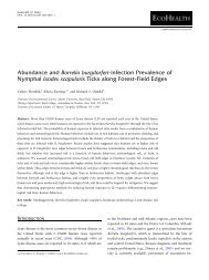
is critical for predicting the effect of engineers on speciesrichness at the landscape scale.Gurney and Lawton (1996) developed a model of thepopulation dynamics of ecosystem engineers that linkedthe production and decay of engineered habitats to thepopulation dynamics of engineers. Specifically, themodel focused on allogenic engineers that must modifytheir habitat to survive, (e.g. beaver damming streamsand pocket gophers digging burrows) as opposed tothose where the engineering activity has no effect on theengineers performance (e.g. hippopotamus forming trailsand buffalo creating wallows). Allogenic engineers arethose engineers that modify the environment by transformingliving or non-living materials from one physicalstate to another primarily by mechanical means (Jones etal. 1994), and as a result create patches that can persisteven if the organism that created them is no longerpresent. Gurney and Lawton (1996) focused primarily onthe conditions for stability of populations of engineers.However, their model also predicted steady state valuesfor the proportion of engineered and unmodifiedhabitats.Here, we modify Gurney and Lawton’s original (1996)model and analyze how the model’s parameters affectthe steady state abundance of different habitat types. Wealso use data collected on the population dynamics of aparticularly well-studied ecosystem engineer, the beaver,to estimate values for several of the model’s parameters.Using these estimated parameter values, we explore theeffects of varying parameters on the relative abundanceof different habitat types.ModelsSimple patch dynamic modelIn the simplest version of the model, patches within alandscape can be found in one of three potential states:potential, active, and degraded. Patches in the potentialstate are transformed into active patches via the processof colonization of the patch by dispersing ecosystemengineers arriving from active patches. Patches aretransformed from the active state to the degraded statewhen the patch is abandoned, and patches change fromdegraded to potential through a process of recovery (Fig.1A, Table 1). If we denote the proportion of patches inthe potential, active, and degraded states at time t by P,A, and D respectively, then we know that1PAD (1)We assume that a unit of active habitat has a constantprobability per unit time of decaying into the degradedstate (d) and that a unit of degraded habitat has aconstant probability per unit time of recovering to thepotential state (r). We further assume that each activepatch generates a constant number of individuals perFig. 1. A) Structure of the simple (3-patch) model and B)complex (4-patch) model of the dynamics of patches in anengineered system. Patches that are actively occupied byengineers are designated A, and decay into degraded patches(D) following abandonment. Degraded patches recover intopotentially habitable patches (P) which are then recolonized toform active patches. In the 4-patch model, if potential patchesare not recolonized, they progress to the fully recovered (F)state.Table 1. Description of the parameters in simple (3-patch) andcomplex (4-patch) models of the dynamics of patches in anengineered system.Parameter Descriptionndrirzunit time that succeed in converting a potential patchinto an active patch (n). Recalling that Eq. 1 allows us tocalculate P t given A t and D t , we can describe thedynamics of this system by two differential equations:dAdt nA(1AD)dAdDdt dArD(2a)(2b)This system has two biologically relevant steady states.One, which we call the zero-engineer state has A* (theproportion of the landscape in the active state atequilibrium)/D*/0 and P*/1. The other, which wecall the finite engineer state, hasA 1 d=n1 d=rPer-patch production rate of new colonistsDecay rate of patches from active (A) to degraded(D) stateRecovery rate of patches from degraded (D) topotential (P) stateImmigration rateRecovery rate of patches from potential (P) state tofully recovered (F) stateDiscrimination of colonists against potential (P)relative to fully recovered (F) patchesD dA rFor this steady state to be biologically meaningful, itmust have A*/0 and D*/0, which in turn requiresn/d/0. This implies that for the engineer to persist,the number of new patches created per unit time mustexceed the patch degradation rate.(3)OIKOS 105:2 (2004) 337

Simple patch dynamic model with immigrationIn the initial formulation of the model, the rate oftransformation of all P patches to A patches is dependenton the abundance of A patches in the landscape.This is the case when dispersing engineers can only arisefrom engineered patches within the system. However, itis conceivable that there are patches in the landscape thatcan support engineers without habitat modification andthus persist indefinitely. For example, beaver live primarilyin ponds that they create by damming streams(converting a patch from P to A). These active coloniesproduce new colonists that disperse and create newactive patches. However, beaver can also live in naturallakes and ponds, producing a source of colonists that isindependent of the number of beaver-created ponds inthe landscape. To address a situation where there is asource of colonists independent of the stock of engineeredpatches, we modify the original model to includean additional constant inflow of immigrants at rate i,thus yielding:dAdt (nAi)(1AD)dA(4a)dDdt dArD(4b)This system has only one biologically meaningful steadystate, at which A* is a solution of(n[1d=r])A 2 (i[1d=r]dn)A10 (5)If all parameters (including i) are assumed to takepositive values, this equation must have exactly onefinite positive solution. Thus, when immigration is addedto the model, the system always has a single finiteengineersteady state but no longer has a zero-engineersteady state.Partial patch recoveryWe now recognize an additional patch state to reflect anadditional stage of recovery from the effects of ecosystemengineering (Fig. 1B). This can occur when ecosystemengineers create patches where recovery rates of thenecessary resource are not equal throughout the patch.For example, beaver can recolonize a meadow site thathas undergone sufficient forest regeneration around theedge of the former pond prior to any woody regenerationwithin the former pond site itself. In this system,patches in the P state represent a recolonisable but notfully recovered state, and patches can additionally existin the fully recovered state. Hence, if we denote theproportion of fully recovered patches in the landscape byF, then1FADP (6)We again assume that a unit of active habitat has aconstant probability per unit time of decaying into thedegraded state (d), that a unit of degraded habitat has aconstant probability per unit time of recovering to thepotential state (r), and that each active patch generates aconstant number of individuals per unit time thatsucceed in converting a potential patch into an activepatch (n). The rate at which A is generated is no longerstrictly dependent on P, but on the sum of (F/zP) wherez represent the degree of discrimination against previouslymodified patches. At this point we assume thatproduction of colonists from active patches is independentof patch history. We also assume that patches in theP state recover at a constant rate per unit time to the Fstate (r). Remembering Eq. 6 allows us to calculate anygiven state variable if we know the other three, so we canrepresent the dynamics of our extended system by:dAdt nA(Fz)dA(7a)dDdt dArD(7b)dPdt rDrPnAzP(7c)The system has two steady states / the zero engineerstate where A*/D*/P*/0 and F*/1, and a finiteengineersteady state, at which A* is the solution of(nz[1d=r])A 2 (r[1d=r]d[1z]nz[1d=n])Ar(1d=n)0 (8)Thus, as long as the patch specific colonization rate isgreater than the degredation rate (n/d) there must be atleast one non-zero positive (real) solution for A*.Beaver as a model systemBeaver are a particularly well-studied example of ecosystemengineers. Beaver have been documented to affectriparian trees (Barnes and Dibble 1986, Nummi 1989,Johnston and Naiman 1990b), biogeochemistry ofstreamwater (Naiman et al. 1986, Margolis et al. 2001)and soil (Johnston et al. 1995), fish populations (Hansonand Campbell 1963, Snodgrass and Meffe 1998), diversityof aquatic invertebrates (McDowell and Naiman1986), birds (Grover and Baldassarre 1995, Nummi andPoysa 1997), and herbaceous plants (Wright et al. 2002),and succession (McMaster and McMaster 2000). Allriparian effects of beaver are the result of their ecosystemengineering activities, with the possible exception ofchanges in the composition of riparian trees, due in partto herbivory. Specifically, these effects are caused by abeaver dam transforming a free-running stream into apond that floods the adjacent riparian zone, or by the338 OIKOS 105:2 (2004)

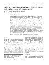
draining of a pond and exposure of accumulatedsediments following abandonment of a site and subsequentdam failure.In the model, beaver ponds with a resident colony areconsidered as active patches (A). Typically, only theoldest pair of beaver in a colony will reproduce,producing on average 3 or 4 young annually (Jenkinsand Busher 1979). Colonies typically consist of an adultpair, yearlings, and kits, with an average size of 5.859/0.61 (SE) individuals (Svendsen 1980). Young beaverdisperse at about 2 or 3 years of age (Jenkins and Busher1979, Svendsen 1980), although if food supplies areplentiful or local population densities are high, as manyas 50% of two-year old beaver can remain at their natalcolony (van Deelen and Pletscher 1996). Dispersaldistances tend to be less than 16 km (Beer 1955, Leege1968), but distances of up to 110 km have been reported(Hibbard 1958). Mortality during dispersal tends to behigh relative to non-dispersing beaver, with mortalityrates of 40% being reported for the 1.5/2.5 year class ofbeaver in Newfoundland (Payne 1984). Birth rates percolony, site fidelity and mortality during dispersal areimportant factors in determining the model parameter n,or the per patch production rate of successful colonists.Although these factors are likely to vary across the rangeof beaver, if one assumes the figures reported above arestandard for beaver across their range, one can estimatea value for n of 0.7 successful immigrants per year.It is also possible that the creation of active patchesmay be affected by the presence of colonies of beaverthat occur in sites that do not require habitat modification.Beaver are known to build lodges on naturallyoccurring lakes and ponds as well as in the banks oflarger rivers without performing any significant engineering.In landscapes where such patches are present,the number of successful colonists that are produced bythese non-engineered sites (i) will influence the rate atwhich new active patches are formed. Although it ispossible that the number of colonists coming from nonengineeredpatches is not constant and might depend onthe number of engineered patches in a landscape, tosimplify analysis of the model, we have assumed aconstant rate of immigration.Over time, active colonies deplete the food resourcesadjacent to the pond, ponds fill with sediment, andresident beaver die eventually leading to abandonment.The rate at which this occurs (d) will be a function ofcolony size, beaver activity, the composition and abundanceof riparian zone trees or other food resources, andsediment loads of dammed streams. Knudson (1962)reported that beaver ponds may remain active for as longas 8/10 years, while in Algonquin Provincial Park,Canada, sites were occupied for an average of 5.89/0.46 (SE) years over a ten year period (Fryxell 2001).Once ponds are abandoned, they develop into wetlandswith variable hydrologic regimes and vegetation composition(Remillard et al. 1987, Johnston and Naiman1990c, McMaster and McMaster 2000, Wright et al.2002). The sites remain in this state (equivalent todegraded, D, patches) until the vegetation in the areaadjacent to the former pond site has recovered to adegree sufficient to support a new beaver colony. Therate at which this transformation from D patches to Ppatches occurs (r) depends on the successional dynamicsof the forests surrounding pond sites.In most areas, once beaver have colonized a site, thesite enters into a pattern of cyclic abandonment andrecolonization. It is relatively rare for a site that has beencolonized by beaver to revert back to a forested riparianzone (equivalent to the F state in the more complexpatch dynamic model, Ives 1942, Remillard et al. 1987,Johnston and Naiman 1990a, Pastor et al. 1993,Terwilliger and Pastor 1999), thus the parameter r islikely to be extremely low in most ecosystems affected bybeaver. The degree to which beaver prefer or avoid sitesthat have been previously colonized relative to forestedriparian zone (z) will again depend on the successionaldynamics of the riparian zone vegetation. In many areas,recently abandoned sites are dominated by species ofSalix, Populus and Alnus, preferred food species ofbeaver (Jenkins and Busher 1979). The situation whereherbivores, such as beaver, create environments favorablefor the growth of early-successional species, which areoften preferred by beaver, has been termed the retardedsuccession hypothesis (Pastor and Naiman 1992). However,it is also possible for beaver foraging to facilitate thedominance of conifers and other late-successional speciesthat are typically avoided as food sources, (theaccelerated succession hypothesis, Fryxell 2001).Furthermore, it has been shown that browsing by beavercan increase rates of phenolic glycoside production inPopulus fremontii (Martinsen et al. 1998). If suchchemical defenses against mammalian herbivory persistor browsing by beaver leads to dominance of nonpreferredspecies, sites that have been previously occupiedby beaver might be avoided.Beaver activity on the Huntington Wildlife Forest(HWF) has been surveyed annually since 1979. TheHWF is a 6000-hectare preserve located in the centralAdirondack Mountains, NY (latitude 44800?N, longitude74813?W). The topography is mountainous withelevations ranging from 457 m to 823 m. Vegetationconsists of mixed northern hardwood and coniferousforest. As part of the Adirondack Long Term MonitoringProject (ALTEMP), all active beaver sites on HWFhave been identified and mapped every fall since 1979.Although the number of colonies has fluctuated overtime (Fig. 2), the number of beaver colonies hasremained relatively constant, particularly since 1990.Although there is some variability in the numbers ofindividuals per colony, colony counts can provide auseful estimate of population sizes for beaver (BergerudOIKOS 105:2 (2004) 339

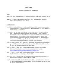
Fig. 2. Number of active beaver colonies on the HuntingtonWildlife Forest (HWF) recorded during annual censuses fromthe period 1979/1998.and Miller 1977). Assuming that beaver populations areclose to steady state in the central Adirondacks, datafrom these surveys can be used to estimate several of theparameters of the model.We estimated d, the rate of decay from A (active) to D(degraded) patches, by calculating the mean period oftime that ponds remained active, considering only pondsthat were colonized after 1979 and abandoned prior to1999. If one assumes that d is distributed exponentially,then the rate of decay is the inverse of the mean age ofthe patch. For the period from 1979/1999, the meantime of occupation for beaver ponds on HWF was 4.8years9/0.34 (SE) yielding an estimate of d/0.21.The production rate of successful colonists per patch(n) is slightly more difficult to estimate. Since beavercolonies occur on natural lakes in HWF, dispersal ofindividuals from patches not created by beaver almostcertainly occurs. However, dividing the number of newlyactive sites in a year by the number of active colonies inthe previous year produces an upper bound for theestimate of n (essentially ignoring the effects of nonengineeringcolonies). For the period from 1980/1999,this technique yields an average estimate of n/0.399/0.03, lower than the value of 0.7 predicted from theliterature.The data from the annual beaver census are insufficientfor estimating the other parameters of the simplepatch dynamic model. Estimating the rate of recoveryfrom degraded (D) to potential (P) patches, r, requiresmeasuring recovery in the forests adjacent to pond sitesas well as determining the minimum requirements forcolonization by beaver. However, the mean time periodthat ponds were abandoned was 4.799/0.35 years,suggesting a minimum value of r/0.21. Estimatingimmigration from non-engineering patches (i) wouldrequire tracking dispersing individuals from suchpatches and determining successful colonization rates.Estimating the additional parameters of the morecomplex patch model is also somewhat challenging.The rate of recovery from previously used sites toforested riparian zone is difficult to estimate, but canbe safely assumed to be extremely low given the raritywith which such transitions have been observed (Remillardet al. 1987, Pastor et al. 1993). We can estimatebeaver relative preference for virgin or fully recoveredversus previously modified patches (z) using data fromthe annual beaver surveys. The ratio of the proportion ofpreviously used available patches that are colonized tothe proportion of virgin habitat colonized in a given yearis an index of habitat preference. Values greater than 1indicate a preference for previously used habitat whilevalues less than 1 indicate preference for virgin habitat.If one assumes that all possible patches on HWF havebeen colonized by the latest year of the beaver survey(1999), one can calculate a lower limit for z. Ignoringyears in which no beaver colonized previously virginhabitat, the mean value of z between 1981 and 1998 is1.21, indicating a slight preference by beaver forpreviously engineered habitat. There is a significanttrend for this estimate of z to decrease over time(F 1,12 /21.32, r 2 /0.66, p/0.0007, Fig. 3), with preferencefor previously modified habitats switching topreference for virgin habitat around 1986.We solved the system of differential equations todetermine the steady state values of the proportions ofthe different habitat types while varying one parameterand holding all other parameters in the model constant.In solutions in which they were held constant we usedthe values of d (0.21), n (0.39), and z (1.21) estimatedfrom annual beaver surveys. We held r constant at 0.25(yielding a mean recovery time from degraded intopotential patches of 4 years), r at 0.01 (yielding a meanrecovery time from potential into fully recovered patchesof 100 years), and i at 0.1.Fig. 3. Log of preference index for fully recovered (F) versuspreviously modified sites (P) for use as sites for colonizationderived from HWF beaver censuses between 1980 and 1998.Untransformed values greater than one indicate a preference forpreviously occupied habitat. The equation for the best fitregression is log (y)/167.44/0.08x.340 OIKOS 105:2 (2004)

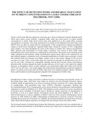
ResultsSimple modelAs d, the decay rate of patches from the active todegraded state, increases, the proportion of the landscapein the P* (potential) state increases in a near linearfashion until d/n, the per-patch production rate of newcolonists, at which point P* reaches a maximum at 1(Fig. 4A). At low values of d, most of the landscape is inthe A (active) state, but the proportion of A* decreasessteadily as d increases, reaching 0 when d/n. Theproportion of D* (degraded) patches in the landscapeshows a unimodal relationship as d increases, representinga trade-off between low production of degradedpatches at low d, and a low supply of active patches athigh d.Varying r, the recovery rate of degraded patches intopotential patches, while keeping the values of the otherparameters constant has no effect on the steady statevalue of P* (Fig. 4B), as potential patches are rapidlytransformed to active patches. As r increases, D*decreases and A* increases, with dominance betweenthe two patch types switching when r/d, representingthe point at which old patches decay more rapidly thannew patches are created.At levels of nB/d, the landscape is at the zero-engineersteady state with P*/1, and A*/D*/0 (Fig. 4C). Asn increases above this point, P* decreases steadily whileA* and D* increase. If dB/r, A* will increase morerapidly than D* and reach a higher value as n increaseswhile if d/r, D* will increase more rapidly.Simple model with immigrationAdding immigration changes the dynamics of the systemquite considerably. Fig. 5A illustrates that increasing dagain causes A* to decrease steadily although, withimmigration, a value of 0 is no longer possible. The moststriking difference is that even with small amounts ofimmigration, P* increases much more slowly with d andat a rate that is far from linear (compared to Fig. 4A).Also, D* only decreases slightly at high values of d ratherthan peaking at low values of d and then decreasing.With immigration, P* is no longer independent of r,but decreases to values near 0 at low values of r (Fig.5B). However, adding immigration does not affect thebasic relationship between r and A* or D*. At lowvalues of n, immigration prevents the system frombecoming fixed at P*/1 and A*/D*/0 (Fig. 5C).Apart from that, the relationship between the steadystate values of the state variables and different values ofn are similar with and without immigration (Fig. 4C,5C), although the responses are dampened with immigration.Fig. 4. Dynamics of steady state values for state variables of thesimple (3-patch) model without immigration in response tochanges in the model parameters. In simulations where theywere held constant, d/0.21 (A), r/0.25 (B), and n/0.39 (C).Although adding immigration to the model alters therelationships between the other parameters and the statevariables, varying the immigration rate itself has arelatively small effect on A* and D* (Fig. 5D). At verylow levels of i, P* increases while A* and D* decrease.Figure 6A shows that at low values of d, addingimmigration has little effect on the steady state values ofOIKOS 105:2 (2004) 341

Fig. 6. Difference between the steady state values for statevariables with (i/0.1) and without immigration. In simulationswhere they were held constant, d/0.21 (A), r/0.25 (B), andn/0.39 (C).Fig. 5. Dynamics of steady state values for state variables of thesimple (3-patch) model with immigration in response to changesin the model parameters. In simulations where they were heldconstant, d/0.21 (A), r/0.25 (B), n/0.39 (C), and i/0.1(D).any of the state variables. At high values of d, the majoreffect of adding immigration is to increase the proportionof D* while decreasing the proportion of P*.Immigration causes the relative abundance of A* andD* to increase and P* to decrease until d/n. At valuesof d/n, the differences between the values of the statevariables with and without immigration begin to decrease.Adding immigration only causes small changes inthe effect of r, on the steady state values of the state342 OIKOS 105:2 (2004)

variables, and this effect is largest at low values of r (Fig.6B). Adding immigration also affects the relationshipbetween n and the steady state values of the statevariables at low values of the parameter, but themagnitude of the effect is much larger (Fig. 6C). Thedifferences between the steady state values of the statevariables in the model with and without immigrationbegin to decrease at n/d. For all values of all threeparameters, the effect of adding immigration (at i/0.1)is to reduce the proportion of P* while increasing theproportion of A* and D*.Partial recovery modelAdding a fourth patch type to the model causes severalimportant changes to the behavior of the model.Increasing d causes A* to decrease steadily and F* toincrease steadily while D* and P* reach a maximum atintermediate values of d (Fig. 7A). Not surprisingly,increasing r causes D* to decrease (Fig. 7B). Interestingly,varying r only results in a slight increase in P*except at low values of r presumably because patches inthe P state are quickly transformed into A accountingfor the increase in A* as r increases. Increasing r has anegative effect on F*, particularly at low values of r. Atvalues of n/d, F* and P* steadily decrease as nincreases while A* and D* increase (Fig. 7C). Increasingr has a negligible effect on A* and D*, and servesprimarily to increase F* while decreasing P* (Fig. 7D).Varying z, the degree of discrimination againstpartially recovered patches relative to fully recoveredpatches, causes the most interesting changes in thesteady state values of the state variables. Increasing z,or causing the engineer to prefer sites in the partiallyrecovered state to fully recovered patches, causes bothA* and D* to increase (Fig. 7E), presumably since itessentially increases the number of patches that areavailable to colonization. Interestingly, increasing zcauses F* to decrease. This is because, as the willingnessof engineers to colonize partially recovered patchesincreases, partially recovered patches tend to be colonizedand converted to active patches before they canfully recover. P* shows a unimodal relationship with z,with a maximum at intermediate values of z. Thisrelationship represents a balance between the directincrease in the rate at which P is converted into A andthe indirect effect of increasing A on the production of P(via an increase in D) as z increases. At both highervalues of d and lower values of n, the peak in P*, occursat lower values of z.Although this model is significantly less analyticallytractable than the simpler models, under certain conditions,the system behaves essentially like the simplesystem discussed above. Specifically, as r approaches 1,particularly at values of z close to (or greater than) 1, theFig. 7. Dynamics of steady state values for state variables of thecomplex (4-patch) model in response to changes in the modelparameters. In simulations where they were held constant, d/0.21 (A), r/0.25 (B), n/0.39 (C), r/0.01 (D), and z/1.21(E).OIKOS 105:2 (2004) 343

Fig. 8. Effect of varying the rate of recovery from partiallyrecovered patches (P) to fully recovered patches (F) and level ofpreferences for previously used versus fully recovered habitat (z)on the difference between the simple (3-patch) model andcomplex (4-patch) model in the steady state proportion of activepatches (A). Values of z greater than one indicate a preferencefor previously used habitat. In all simulations, d/0.21, r/0.25and n/0.39.values of the state variable at steady state approach thoseof the simple model with the same parameters (Fig. 8).DiscussionModel predictionsThe three versions of the model presented here producequantitatively different predictions about the proportionof engineered landscapes in different habitat types as theparameters are varied. However, all three models agreeon several important qualitative predictions aboutengineered landscapes (Table 2). Landscapes will tendto have large proportions of active patches (A) whenecosystem engineers are efficient in their resource use,producing many new colonists while only graduallydegrading the resources of the patch, and when resourcerenewal occurs rapidly after engineers abandon a site.Engineers that create landscapes dominated by abandoned(D) patches would produce large numbers ofcolonizers by rapidly depleting the resource levels of apatch, and leaving abandoned patches that recover veryslowly. In most respects, the proportion of potential sitesin the simple model (P) reacts to changes in theparameters in a manner similar to the proportion offully recovered sites (F) in the more complex model.Ecosystem engineers that create patches that producefew new colonizers and are abandoned quickly, yetrecover rapidly should create landscapes dominated bythese fully recovered patch types. In landscapes bestdescribed by the partial recovery model, partiallyrecovered patches (P) will be most abundant whenabandoned patches rapidly recover to a state sufficientto allow recolonization, but only slowly regenerate to thefully recovered state.In many cases, sites currently used by ecosystemengineers, and those recently abandoned are easilydistinguished from patches that have not been modifiedby engineers. For example, pocket gophers form distinctmounds of loose soil in many prairie ecosystems (Huntlyand Inouye 1988), grizzly bears create extensive patchesof tilled soil in alpine meadows while foraging for lilybulbs (Tardiff and Stanford 1998), tilefish and grouperexcavate marine sediments (Coleman and Williams2002), and leaves occupied by shelter-building Gelechiidcaterpillars are strikingly tied together, Lill and Marquis2003. Because these states are readily identifiable, itshould be feasible to compare the relative abundance ofdifferent patch types in landscapes where the sameengineer operates, but where values of the parametersare likely to be different (e.g. predation risk is higherthus lowering the number of successful colonizers, orproductivity is higher, thereby speeding up recovery fromabandoned sites). Such an analysis would serve as acritical test of whether these models successfully capturethe relationship between the population dynamics of anecosystem engineer and the dynamics of the patches itcreates.Differences between modelsAdding a fourth patch type to represent habitat that ispartially recovered, yet still capable of being engineereddoes not alter the fundamental patch dynamics of themodel. In both the original and partial recovery versionsof the model, the proportion of the landscape that willbe in the active and degraded states at steady state reactssimilarly to changes in the parameters d, r, and n.Furthermore, the steady state proportion of potentialpatches (P) in the simple model behaves similarly to thesteady state proportion of fully recovered patches (F) inthe complex model with respect to changes in d and nTable 2. Summary of the parameter combinations that lead to high relative abundance of each of the patch types in the threemodels.Patch type 3-Patch model without immigration 3-Patch model with immigration 4-Patch modelA / r, n;¡/ d / r, n;¡/ d / r, n;¡/ dD / n; ¡/ r; intermediate d / d, n;¡/ r / n; ¡/ r; intermediate dP / d; ¡/ n / d, r; ¡/ n, i / r; ¡/ n, r; intermediate d, zF N.A. N.A. / d, r;¡/ r, n,z344 OIKOS 105:2 (2004)

(and to a lesser degree, to changes in r). Given the addeddifficulty of determining analytical solutions to the morecomplex model and estimating an additional parameter,the benefits of the four-patch model seem limited. Onlyin systems where there are important differences betweenpartially recovered and fully recovered patches, e.g.between the vegetation of beaver meadows and riparianzone forest (Terwilliger and Pastor 1999, Wright et al.2002), would it be worthwhile to model the patchdynamics of the system using the four-patch model.Immigration, either from outside the boundaries ofthe system, or from patches within the system whereengineers can reproduce without having to modifyhabitat has the potential to alter the dynamics of thesystem. With even small amounts of immigration, thezero engineer steady state is no longer possible. Theeffects of immigration will be highest when engineersreside in a patch for a short time (i.e. high d), producefew successful colonizers (i.e. low n), and where degradedpatches recover rapidly (i.e. low r).Model parametersWhile the relative abundance of different patch types in alandscape can be relatively easy to determine, estimatingthe parameters of the model is somewhat more challenging.Although we were able to estimate some of themodel parameters indirectly using data on beaverpopulations and patch transitions in the central Adirondacks,we are unaware of any data set that wouldallow independent estimation of all of the model’sparameters. Future studies of the effects of ecosystemengineers on patch dynamics would benefit by structuringtheir questions in a manner that would allowinvestigators to estimate the parameters of these models.Of all the parameters, d, or the rate at which activesites are abandoned, is likely to be the easiest to estimate.Careful long-term monitoring of patch use by engineerswill yield average lifetimes of engineered patches, whichcan be converted into probabilities of patch decay. Ingeneral, organisms that exhaust patch resources graduallyrelative to the rate of resource renewal, e.g. moundbuildingdesert shrubs (Shachak et al. 1998), should tendto create patches with lower values of d than organismsthat are short-lived, e.g. leaf-tying caterpillars (Lill andMarquis 2003), or that use the resources in engineeredpatches much more rapidly than they are replenished.Estimating the number of successful colonists producedper engineered patch (n) is a bit more challenging.It can be inferred by dividing the number of newlyformed patches by the number of active patches at theprevious time step. However, independent measurementof n requires determining two variables: the number ofdispersers produced per engineered patch, and rate atwhich dispersers successfully establish new patches. Thefirst variable will be a function of birth rates and theprobability of individuals to leave their natal patch. Thesecond variable is a function of mortality rate duringdispersal and the probability that dispersing individualswill establish new colonies. In general, ecosystem engineerswith high fertility, low natal site fidelity, and lowmortality during dispersal should have high values of n.The rate at which abandoned patches recover intopotential patches (r) is probably the most difficult toestimate independently. This is because the resourcesnecessary for an engineer to recolonize a patch are likelyto accumulate steadily over time. Determining when thenecessary resources reach the critical level that separatesdegraded patches from potential patches requires athorough knowledge of the requirements of the ecosystemengineer. Furthermore, the level to which criticalresources are depleted in recently abandoned patches islikely to vary, thus the time needed for a degraded patchto recover will vary, even if recovery rates are constantacross the landscape. In general, engineers with lowresource requirements and systems with high resourcesupply rates should have high values of r.In systems where dispersing engineers are produced inpatches that have not been modified by the ecosystemengineer, one must differentiate between the proportionof successful colonists that are produced in nonengineeredpatches (i) and the proportion of coloniststhat are produced in engineered patches (n). If birth ratesare the same in the two patch types and individuals fromengineered and non-engineered patches have identicalprobabilities of successfully producing new patches, therelative importance of n and i in controlling theproportion of active patches will depend on the relativeabundance of active engineered and active nonengineeredpatches in the landscape. If however, birthrates or successful dispersal rates differ between engineeredand non-engineered patches, estimating i willrequire accurate measurements of birth rates in andsuccessful dispersal from non-engineered sites that containengineers.Estimating the rate at which partially recoveredpatches recover fully (r) (i.e. from P to F) has similarchallenges to estimating recovery rates from degradedpatches to potential patches (i.e. r). Tracking patchesover time allows estimates of the amount of timerequired from abandonment to full recovery (assumingone can set the criteria that determine full recovery).However, such an analysis cannot determine how muchof the recovery time is spent in the degraded state versusthe potential state. Independent estimation of r wouldagain require detailed understanding of the criteria usedby engineers when selecting sites, and may requiremeasurements difficult to obtain using typical methodsof surveying habitat such as the nutritional quality ofdifferent plants species (Martinsen et al. 1998). Despitethese difficulties in estimating r, we hypothesize thatOIKOS 105:2 (2004) 345

systems where engineers perform qualitative transformationof the physical state of the patches they modify, e.g.beaver transforming terrestrial patches into aquaticpatches, are likely to have much lower values for r thansystems where the engineers only perform quantitativetransformations of habitats, e.g. shrub mounds increasingwater infiltration rates in desert soils (Shachak et al.1998).In systems where engineers can recolonize patchesbefore they have fully recovered, one must also determinethe degree to which engineers prefer or avoidpartially recovered patches relative to fully recoveredpatches (z). As illustrated above with data from annualbeaver surveys, if one can determine the total number ofpatches available in a landscape, this metric is notdifficult to estimate. It requires calculating the degreeto which new patches are formed in each of the twohabitat types (partially and fully recovered) relative totheir availability. In general, most systems are likely tohave values of z less than one, indicating that engineersprefer fully recovered to partially recovered patches.However, as suggested by the data from the annualbeaver surveys, it is possible for positive feedbacks tooccur whereby conditions in abandoned sites are favorablefor the establishment of species that are preferred tothose found in fully recovered sites.Implications for beaverOver the past 20 years, beaver populations on HWF haveremained relatively constant. The large jump in observedcolonies between 1985 and 1986 is due, at least in part, toan increase in the area covered during annual beaversurveys (C. Demers, pers. com.). Since 1989, the numberof active colonies on HWF has fluctuated relatively littleamong years. These data are consistent with theassumption that the beaver populations and the patchdynamics of beaver-modified habitats are at steady state.Since we were unable to independently estimate all ofthe model’s parameters, we could not directly test themodel’s predictions as to the relative abundance ofdifferent patch types in the landscape. Nevertheless,analyzing the model’s behavior using parameters estimatedfrom the annual beaver surveys reveals someinteresting features of the system. Our estimate of thenumber of successful colonists produced per engineeredpatch (n) is doubtless an overestimate. The calculation ofn ignored the role of colonists that originated from nonengineeredpatches (e.g. natural lakes). Even with theoverestimate, our estimate of n (0.39) is close to ourestimated value of the decay rate of active patches (d/0.21). In both versions of the model without animmigration term, engineers cannot persist in a systemwhere the decay rate, d, is greater than the patch creationrate, n. Thus, immigration, either from outside thesystem or from non-engineered patches, is likely to beimportant in maintaining beaver populations in thecentral Adirondacks. The habitat within the HWF isessentially identical to the surrounding area, so there isno reason to expect that HWF is receiving significantlymore dispersing beaver than it is losing through emigration.This points to the central importance of colonies oflake-dwelling beaver in maintaining the patch dynamicsof beaver-modified habitats.If the estimates of the model parameters are correct, itwould suggest that the relative abundance of differenthabitat types should be most sensitive to changes in thedecay rate of active patches (d), and the successfulcolonization rate (n). While decay rates depend primarilyon the rate at which beaver use up resources in a site andare unlikely to vary significantly over time, successfulcolonization rates could vary significantly depending onpredation rates during dispersal. Wolf reintroduction tothe Adirondacks or increasing populations of coyotescould potentially increase predation during dispersal,thereby lowering n. Based on our parameter estimates,such changes in n would lead to large decreases in theproportion of active ponds and young meadows withconcomitant increases in old meadows with welldevelopedsurrounding forests. Older meadows tend tobe much dryer than new meadows and as a result,contain a quite different community of wetland plants(Wright et al. 2003). Thus, changes in n due to increasedmortality during dispersal could have strong effects ondiversity at the landscape-scale.The decline in beaver preference for previously usedsites (z) over time is somewhat counterintuitive. If thereis variability in site quality, and beaver first selectoptimal sites (Howard and Larson 1985), one mightassume that beaver would prefer to re-use high qualitysites rather than colonize poorer quality sites, leading tohigher values of z. The relationship is in part due to theassumption that all possible sites had been colonized bythe time of the last survey. However, if we assume thatonly half of the available sites had been colonized in1999, the decline over time, while weaker, still remainssignificant (F 1,11 /25.14, r 2 /0.68, p/0.0004). It maybe that patches that are repeatedly used begin to declinein quality over time, particularly if repeated browsing bybeaver leads to dominance by non-preferred species suchas conifers or other late-successional species. There issome evidence of such an accelerated succession dynamiccaused by beaver in Algonquin Provincial Park(Fryxell 2001), thus it is certainly possible that this isoccurring in the Adirondacks as well. If so, this wouldcause beaver to increasingly avoid previously usedpatches over time, leading to the observed lower valuesof z. The model predicts that decreases in z should leadto decreased proportions of active ponds and newmeadows and increased proportions of old meadows,mirroring the effects of lower n.346 OIKOS 105:2 (2004)

ConclusionsThe set of models developed here helps link thepopulation dynamics of ecosystem engineers to thedynamics of the patches that they create. By predictingthe relative abundance of engineered and unengineeredpatches in a landscape, it has the potential to serve as animportant tool in determining the effects of ecosystemengineers on ecosystem structure and function at thelandscape scale. Application of the model to a populationof beaver in the central Adirondack Mountainssuggests that because successful colonization rates arelow and site abandonment rates are high, the populationpersistence may depend on dispersers from beavercolonies in unmodified patches such as natural lakes.Although we are not aware of any data set that wouldallow for complete parameterization of the model,analysis of the model suggests a number of possibletests of its structure and assumptions. The model makesnumerous testable predictions about how the distributionof patch types in a landscape should change inresponse to changes in the population dynamics ofengineers or the recovery rate of patches after theyhave been abandoned. Furthermore, by combining thismodel with an understanding of how ecosystem engineeringaffects diversity at the landscape scale, we nowhave the tools to relate the population dynamics of anorganism to patterns of landscape-level diversity.Acknowledgements / The authors gratefully acknowledge theAdirondack Ecological Center for access to the long-term dataset on beaver dynamics of the Huntington Wildlife Forest.Special thanks to C. Demers and R. Sage for their help inorganizing and maintaining this valuable resource. A. Flecker, P.Marks, B. Goodwin, R. Root and P. Nummi provided manyuseful comments and suggestions for improving the manuscript.This work was funded by Sigma Xi, the Laurel Foundation, theKieckhefer Adirondack Fellowship, the Institute of EcosystemStudies, and an NSF GRT for Human AcceleratedEnvironmental Change. This study is a contribution to theInstitute of Ecosystem Studies.ReferencesBarnes, W. J. and Dibble, E. 1986. The effects of beaver inriverbank forest succession. / Can. J. Bot. 66: 40/44.Beer, J. R. 1955. Movements of tagged beaver. / J. Wildl.Manage. 19: 492/493.Bergerud, A. T. and Miller, D. R. 1977. Population dynamics ofNewfoundland beaver. / Can. J. Zool. 55: 1480/1492.Coleman, F. C. and Williams, S. L. 2002. Overexploiting marineecosystem engineers: potential consequences for biodiversity./ Trends Ecol. Evol. 17: 40/43.Collins, S. L. and Uno, G. E. 1983. The effect of early springburning on vegetation in buffalo wallows. / Bull. TorreyBot. Club 110: 474/481.Crooks, J. A. 2002. Characterizing ecosystem-level consequencesof biological invasions: the role of ecosystemengineers. / Oikos 97: 153/166.Fryxell, J. M. 2001. Habitat suitability and source-sinkdynamics of beavers. / J. Anim. Ecol. 70: 310/316.Grover, A. M. and Baldassarre, G. A. 1995. Bird speciesrichness within beaver ponds in south-cenral New York./ Wetlands 15: 108/118.Guo, Q. 1996. Effects of bannertail kangaroo rat mounds onsmall-scale plant community structure. / Oecologia 106:247/256.Gurney, W. S. C. and Lawton, J. H. 1996. The populationdynamics of ecosystem engineers. / Oikos 76: 273/283.Hanson, W. D. and Campbell, R. S. 1963. The effects of poolsize and beaver activity on distribution and abundance ofwarm-water fishes in a north Missouri stream. / Am. Midl.Nat. 69: 136/149.Hibbard, E. A. 1958. Movements of beaver transplanted inNorth Dakota. / J. Wildl. Manage. 22: 209/211.Howard, R. J. and Larson, J. S. 1985. A stream habitatclassification system for beaver. / J. Wildl. Manage. 49:19/25.Huntly, N. J. and Inouye, R. S. 1988. Pocket gophers inecosystems: patterns and mechanisms. / BioScience 38:786/793.Ives, R. L. 1942. The beaver/meadow complex. / J. Geomorph.5: 191/203.Jenkins, S. H. and Busher, P. E. 1979. Castor canadensis./ Mammalian Species 120: 1 /8.Johnston, C. A. and Naiman, R. J. 1990a. Aquatic patchcreation in relation to beaver population trends. / Ecology71: 1617/1621.Johnston, C. A. and Naiman, R. J. 1990b. Browse selection bybeaver: effects on riparian forest composition. / Can. J. For.Res. 20: 1036/1043.Johnston, C. A. and Naiman, R. J. 1990c. The use of ageographic information system to analyze long-term landscapealteration by beaver. / Landscape Ecol. 4: 5 /19.Johnston, C. A., Pinay, G., Arens, C. et al. 1995. Influence ofsoil properties on the biogeochemistry of a beaver meadowhydrosequence. / Soil Sci. Soc. Am. J. 59: 1789/1799.Jones, C. G., Lawton, J. H. and Shachak, M. 1994. Organismsas ecosystem engineers. / Oikos 69: 373/386.Jones, C. G., Lawton, J. H. and Shachak, M. 1997. Positive andnegative effects of organisms as physical ecosystem engineers./ Ecology 78: 1946/1957.Knudson, G. J. 1962. Relationship of beavers to forests, troutand wildlife in Wisconsin. Tech. Bull. No. 25. / WisconsinConserv. Dept.Leege, T. A. 1968. Natural movements of beavers in southeasternIdaho. / J. Wildl. Manage. 32: 973/976.Lill, J. T. and Marquis, R. J. 2003. Ecosystem engineering bycaterpillars increases insect herbivore diversity on white oak./ Ecology 84: 682/690.Margolis, B. E., Castro, M. S. and Raesly, R. L. 2001. Theimpact of beaver impoundments on the water chemistry oftwo Appalachian streams. / Can. J. Fish. Aquat. Sci. 58:2271/2283.Martinsen, G. D., Driebe, E. M. and Whitham, T. G. 1998.Indirect interactions mediated by changing plant chemistry:beaver browsing benefits beetles. / Ecology 79: 192/200.McDowell, D. M. and Naiman, R. J. 1986. Structure andfunction of a benthic invertebrate stream community asinfluenced by beaver (Castor canadensis). / Oecologia 68:481/489.McMaster, R. T. and McMaster, N. D. 2000. Vascular flora ofbeaver wetlands in western Massachusetts. / Rhodora 102:175/197.Naiman, R. J., Melillo, J. M. and Hobbie, J. E. 1986. Ecosystemalteration of boreal forest streams by beaver (Castorcanadensis). / Ecology 67: 1254/1269.Nummi, P. 1989. Simulated effects of the beaver on vegetation,invertebrates and ducks. / Ann. Zool. Fenn. 26: 43/52.Nummi, P. and Poysa, H. 1997. Population and communitylevel responses in Anas-species to patch disturbance causedby an ecosystem engineer, the beaver. / Ecography 20: 580/584.OIKOS 105:2 (2004) 347

Pastor, J. and Naiman, R. J. 1992. Selective foraging andecosystem processes in boreal forests. / Am. Nat. 139: 690/705.Pastor, J., Bonde, J., Johnston, C. A. et al. 1993. Markoviananalysis of the spatially dependent dynamics of beaverponds. / Lectures Math. Life Sci. 23: 5/27.Payne, N. F. 1984. Mortality rates of beaver in Newfoundland./ J. Wildl. Manage. 48: 117/126.Remillard, M. M., Gruendling, G. K. and Bogucki, D. J. 1987.Disturbance by beaver (Castor canadensis) and increasedlandscape heterogeneity. / In: Turner, M. G. (ed.), Landscapeheterogeneity and disturbance. Springer-Verlag, pp.103/122.Shachak, M., Sachs, M. and Moshe, I. 1998. Ecosystemmanagement of desertified shrublands in Israel. / Ecosystems1: 475/483.Snodgrass, J. W. and Meffe, G. K. 1998. Influence of beavers onstream fish assemblages: effects of pond age and watershedposition. / Ecology 79: 928/942.Svendsen, G. E. 1980. Population parameters and colonycomposition of beaver (Castor canadensis) in southeastOhio. / Am. Midl. Nat 104: 47/56.Tardiff, S. E. and Stanford, J. A. 1998. Grizzly bear digging:effects on subalpine meadow plants in relation to mineralnitrogen availability. / Ecology 79: 2219/2228.Terwilliger, J. and Pastor, J. 1999. Small mammals, ectomycorrhizae,and conifer succession in beaver meadows. / Oikos85: 83/94.van Deelen, T. R. and Pletscher, D. H. 1996. Dispersalcharacterisitics of two-year-old beavers, Castor canadensis,in western Montana. / Can. Field Nat. 110: 318/321.Wright, J. P., Jones, C. G. and Flecker, A. S. 2002. An ecosystemengineer, the beaver, increases species richness at the landscapescale. / Oecologia 132: 96/101.Wright, J. P., Flecker, A. S. and Jones, C. G. 2003. Local versuslandscape controls on plant species richness in beavermeadows. / Ecology 84: 3162/3173.348 OIKOS 105:2 (2004)