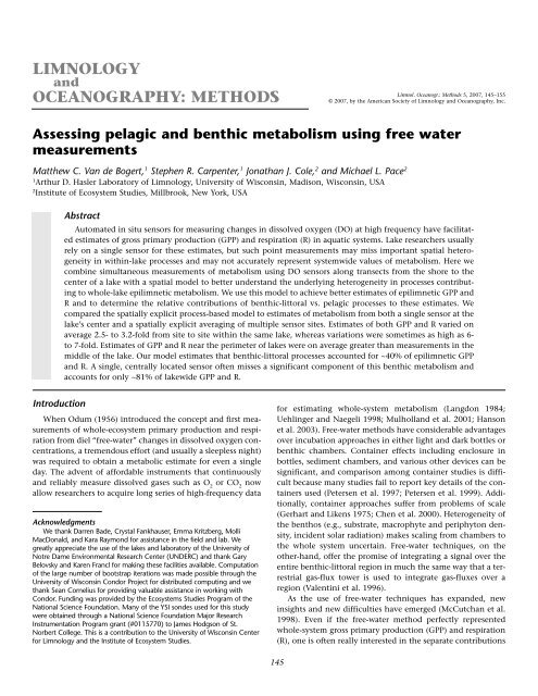
Matthew C. Van de Bogert, Stephen R. Carpenter, Jonathan J. Cole ...

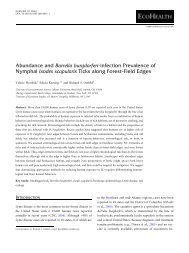
Van de Bogert et al.Benthic and pelagic metabolismFig. 1. Conceptual diagram of a spatial sonde deployment. At eachsonde site (x i) the sensor detects changes in dissolved O 2due to anunknown mixture of benthic and pelagic processes occurring in themixed layer of the lake. In the absence of horizontal dispersion, in shallowwater (where z < z mix) both benthic and pelagic processes would affectthe local sensor. In deep water (where z > z mix) only pelagic processeswould affect the local sensor. At all sites horizontal dispersion tends tohomogenize the O 2signals. Under the right conditions the spatial profilesof dissolved oxygen changes over a transect of sonde sites (x 1to x 6) canbe used to separately compute the benthic contributions to GPP and R.of benthic and pelagic habitats to this whole (Vadeboncoeuret al. 2003). These contributions are sometimes obtained bymeasuring the metabolism of the whole and one of the parts(using bottles or chambers and their associated uncertainties)and inferring the other component by difference (Naegeli andUehlinger 1997; Fellows et al. 2001; Carpenter et al. 2005).However, it is not clear whether free-water techniques actuallymeasure the metabolism of the whole system or some part ofit. To date, most estimates of whole-system metabolism haverelied on single sensors in the middle of the pelagic region.However, dissolved oxygen sensors placed in different habitatsin both rivers (Caraco and Cole 2002) and lakes (Lauster et al.2006) yield estimates of metabolism that vary with location.In both of those studies, oxygen concentrations were moredynamic in shallow, littoral habitats than in open water. If asingle measurement location were able to provide a completeintegration of whole-ecosystem processes, we would notexpect to see different estimates among sites.Lauster et al. (2006) found that differences in bottle (planktonic)estimates of metabolism between pelagic and littoralhabitats were relatively small, suggesting that planktonicmetabolism was nearly evenly distributed throughout the epilimnion.They also found that although differences were greatestnear-shore, free-water metabolism estimates were greaterthan bottle estimates for both the littoral and pelagic habitats.Lauster et al. (2006) attribute the higher estimates of pelagicmetabolism using the free-water method to benthic sourceswhich are not accounted for by bottle methods. Therefore, afree-water estimate of metabolism from the center of a lake mayinclude some portion (but not necessarily all) of the benthic-littoralsignal. Although the free-water method integrates all signalsthat reach a sensor, the challenge is determining howmuch of the benthic or pelagic signals reach any given location.If localized benthic-littoral processes contribute to wholelakemetabolism in addition to spatially less variable planktonicprocesses, metabolism as measured by free-water methodsshould be greatest near shore (planktonic and benthicprocesses) and lowest at the center of the lake (planktonicprocesses plus advection of some portion of the benthic signal)(Fig. 1). The degree to which measurements near shore arehigher than measurements at the center depends on the magnitudeof the benthic signal as well as the degree of horizontalmixing. Given time-series of measurements at only twolocations, even if one is near shore and the other at the centerof the lake, it is not possible to determine how much of themetabolic signal is derived from benthic sources because thereare two unknown factors: the magnitude of benthic metabolismand the degree of advection from the littoral zone to thepelagic. Several series of measurements along a transect, however,might allow one to simultaneously estimate the rate ofhorizontal advection and partition the metabolism signal intobenthic and pelagic sources. Here we use continuous freewatermeasurements of dissolved oxygen at several locationsalong a littoral-pelagic transect to (1) assess the variation inmetabolism estimates among measurement locations, (2) estimatewhole-lake epilimnetic metabolism based on spatiallyexplicit volume-weighted averages of individual measurements,and (3) develop a spatially explicit model of wholelakeepilimnetic metabolism that partitions the whole-lake estimateinto benthic and pelagic components.Materials and proceduresData for this study were collected from Peter Lake, locatedat the University of Notre Dame Environmental Research Center(UNDERC) near Land O’Lakes, Wisconsin, USA, over thecourse of two summers (2002 and 2003). Peter Lake is a 2.5-hacircular lake with a mean depth of 6 m, a maximum depth of19 m, and an upper mixed layer during summer stratificationof approximately 3 m (Carpenter and Kitchell 1993). In 2002,Peter Lake was fertilized with nitrogen and phosphorus toincrease primary production (Carpenter et al. 2005). As a consequenceof the added nutrients, average phytoplanktonbiomass increased 10-fold in 2002 relative to other years. Wepresent data for both 2002 (fertilized) and 2003 (not fertilized).Dissolved oxygen and temperature were measured usingYSI model 600XLM multiparameter sondes calibrated invapor-saturated air before each deployment. Each deploymentconsisted of 4 to 6 sondes placed within the epilimnion alonga linear transect from the shore to the middle of the lake.Approximately half of the sondes from any deployment werewithin the littoral zone and half in the pelagic. The sondeclosest to shore was placed at a distance from shore where thewater depth was approximately 1 m. Measurements of temperatureand dissolved oxygen were recorded every 5 min at a146

Van de Bogert et al.Benthic and pelagic metabolismdepth of 0.7 m. Deployments lasted from 5 to 10 days, afterwhich the sondes were brought back to the lab to be cleanedand prepared for the next deployment.We followed YSI’s guidelines for deployment and calibration(YSI Environmental, Technical Note #610, www.ysi.com).Briefly, our procedures were as follows. Before each deploymentwe reconditioned the surface of the probe (if necessary)and replaced the dissolved oxygen membrane. Proper probefunctioning was tested using YSI’s suggested diagnostics. Theprobe was initialized to log every 5 min and placed in watersaturatedair to allow the membrane to relax to a stable state.After the membrane had relaxed (4–8 h, verified by stable dissolvedoxygen readings), we calibrated the sensor to the ambientbarometric pressure. Sondes were kept in the laboratorywhile logging data for a minimum of 2 additional hours inwater-saturated air. These predeployment data were used toverify, and correct if necessary, the initial calibration. Uponretrieval (5–10 days later), probes were again placed in watersaturatedair and allowed to log an additional 2–4 h at a stabletemperature. These postdeployment data were used to determinethe drift of the sensor. We corrected the data assumingany drift occurred linearly over the course of the deployment.On average, sonde drift (± 1 SD) was 0.043 ± 0.042 mg L –1 d –1 .Before deploying the transects, we assessed sonde-to-sondevariability by allowing all 6 sondes to simultaneously collectdata from the center of Peter Lake for 5 days. These data wereindependently corrected for drift and used with the modelsdescribed below to obtain daily estimates of metabolism (GPPand R) for each sonde. These estimates were used to determinebaseline sonde-to-sonde variability.Because the oxygen sensors were located within the epilimnionof a strongly stratified lake, we assume they did notmeasure metabolism occurring below the mixed layer. Thisassumption is supported by tracer additions in Peter Lake andcalculations of a vertical mixing coefficient based on heat fluxcalculations. In a previous study, lithium bromide (LiBr) addedto the epilimnion of Peter Lake in May of 1993 was notdetectable below the thermocline over the entire summerstratified season (Cole and Pace 1998). Calculation of masstransfer of oxygen across the thermocline based on the equationsof Chapra (1997) indicates that 3.5 mg O 2m –2 d –1 may belost to the hypolimnion. This amounts to approximately0.04% of the standing stock per day and is less than 0.50% ofthe magnitude of the daily change in epilimnetic dissolvedoxygen concentration. Similarly, Gelda and Effler (2002)accounted for vertical transport of O 2in their metabolismmodels and concluded that this component was unimportantand could be ignored. Therefore, we assume exchange acrossthe thermocline over any given 24-h period is negligible, andfor the purposes of our analyses, whole-lake metabolism refersto horizontal integration of benthic-littoral and pelagicprocesses within the epilimnion and not vertical integrationof all stratification layers. This assumption is not valid for alllakes and all time periods; exchange of O 2across the thermoclinemay need to be accounted for in other circumstancesand could be incorporated into the modeling framework presentedbelow.Photosynthetically active radiation was measured using amechanical pyranograph in 2002 and a Li-COR quantum sensorin 2003. The mechanical pyranograph provided estimatesof total daily radiation, whereas the Li-COR sensor loggedradiation every 5 min. To estimate PAR received every 5 minfrom the 2002 data, the total daily PAR values were partitionedaccording to the potential irradiance curve on a cloudless dayusing the equations of Iqbal (1983). In 2003, wind speeds at 2 mabove the water surface were measured using an R.M. Younganemometer. Five-minute wind speed averages, as well as minimumand maximum values, were recorded with a CampbellScientific 6250 data logger.Site-specific metabolism—To estimate lake metabolism at eachsite, we fitted a simple model to the time series of dissolvedoxygen concentration measured at 5-min intervals. For a singlesonde at a given time, the rate of change of dissolved oxygenconcentration is the result of metabolism and exchange withthe atmosphere.dY= GPP− R+D(1)dtAll symbols in this equation and below are defined in Table 1.Over a short interval, such as the 5-min interval between sondemeasurements, the solution of equation 1 is approximatelyY = Y + ( GPP − R + D)Δtt+ 1 tTo estimate GPP and R from our data, we modified equation2 to account for irradiance and diffusion rate in each 5-mintime interval:Y = Y + GPP24(3)PAR× PAR − R24Δt + D Δt + Zt+ 1 t t t t24Given estimates of the parameters GPP24 and R24, equation 3predicts the next oxygen concentration using measurementsof PAR tand PAR24 and the exchange rate of oxygen with theatmosphere. For a 5-min time interval Δt, the diffusive flux D twas computed asD k ([ O ] − Y )2 SAT , t t=(4)tzwhere [O 2] SAT,tis the concentration of dissolved oxygen inequilibrium with the atmosphere which was calculated at eachtime step from temperature data and the equation of Weiss(1970) and corrected for barometric pressure according to theequations in USGS Water Quality Technical Memoranda#81.11 and #81.15 (United States Geological Survey 1981a;1981b). The coefficient k was computed from the Schmidtnumber (Sc) and the gas piston velocity corresponding to aSchmidt number of 600 (k 600).1−⎛ Sc ⎞ 2k = k(5)600⎝⎜ 600⎠⎟The Schmidt number is dependent on water temperatureand was calculated at each time step using the O 2-specificequation of Wanninkhof (1992). For this analysis, we used a(2)147

Van de Bogert et al.Benthic and pelagic metabolismTable 1. Definition of symbols used in the models.Symbol Definition Unitsa shape parameter (vertical stretch) for the dimensionlessinverse tangent functionA Bratio of benthic area to lake surface area dimensionlessb shape parameter (horizontal shift) for the dimensionlessinverse tangent functionD instantaneous rate of diffusion between mmol m –3 d –1lake and atmosphereGPP instantaneous rate of gross primary mmol m –3 d –1productionGPP24 daily rate of gross primary production mmol m –3 d –1GPP bdaily rate of benthic gross primary mmol m –2 d –1productionGPP pdaily rate of planktonic gross primary mmol m –3 d –1productionk coefficient of gas exchange m d –1k 600coefficient of gas exchange for a gas with m d –1a Schmidt number of 600m xproportion of metabolism (GPP or R) from dimensionlessbenthic sources sensed by a sondeplaced at distance x from shorePAR photosynthetically active radiation on the μmol m –2 Δt –1lake surface over a 5-min intervalPAR24 daily photosynthetically active radiation μmol m –2 d –1on the lake surfaceR instantaneous rate of whole ecosystem mmol m –3 d –1respirationR24 daily rate of whole ecosystem respiration mmol m –3 d –1R bdaily rate of benthic respiration mmol m –2 d –1R pdaily rate of planktonic respiration mmos m –3 d –1t time dY dissolved oxygen concentration μMz xdepth of water in the epilimnion at mlocation xZ autocorrelated model error μMΔt small interval dε model error corrected for autocorrelation μMϕ autocorrelation coefficient dimensionlessconstant value for k 600of 0.4 m d –1 , which is within the rangeof estimates based on wind, CH 4flux measurements, and anSF 6addition to this lake (Bade and Cole 2006). Finally, theareal diffusive flux is divided by the epilimnion depth, z, toexpress the value in volumetric units.The prediction error Z tis autocorrelated, and an autocorrelationcorrection is computed asZ= ϕZ+ εt t−1tTo estimate the parameters GPP24 and R24, we minimizedthe normal negative log likelihood of the Z t(Hilborn andMangel 1997). To determine the autocorrelation coefficient, ϕ,we then minimized the normal negative log likelihood of the ε t.(6)Table 2. Steps in bootstrappingStepDescription1) Fit model Y = f( X, θ)+ ε Determine nominal set of parameters, θ,by minimizing the normal negativelog likelihood of the ε. Computepredictions as Yˆ = f( X, θ).Save Ŷ , θ, and ε.2) Bootstrapping loop2a) Compute pseudo- Randomly sample, with replacement, theobservationsε as ε R. Create pseudo-observationsas Y = Y ˆ + ε .PR2b) Refit model Find new set of parameters, θ B, byminimizing the normal negative loglikelihood of the ε R. Save bootstrapestimates, θ B.2c) Repeat Return to 2a and repeat 10,000 times.3) Compute Statistics Find mean, standard deviation, confidenceintervals, covariance matrix, and soon, for bootstrap estimates of theparameters, θ B.Minimization was computed using the fminsearch function ofMatlab (v. 7). We computed 95% confidence intervals of theparameters by bootstrapping with 10,000 iterations (Efron andTibshirani 1993). Estimates of GPP24 and R24 were computedfor each 24-h period beginning at sunrise as calculated fromthe latitude of Peter Lake and the declination of the sun oneach day (Hartmann 1994).Site-specific estimates of metabolism obtained by fittingequations 3 and 6 to the data make no assumptions aboutsource (benthic or pelagic) of the metabolic fluxes. The estimatesof GPP24 or R24 represent the sum of the processesaffecting the concentration of oxygen at that locationregardless of whether they are benthic or pelagic. We usedthese site-specific estimates in two ways. First, on all days, wecalculated spatially explicit volume-weighted estimates ofwhole-lake GPP and R and compared these to estimates madeby a single sensor at the middle of the lake. Second, weapplied, when possible, a model of whole-lake metabolism tocalculate the separate contributions of benthic and pelagicprocesses to GPP and R.Spatially explicit volume-weighted estimate of whole lakemetabolism—For each of the 40 dates on which we measuredfree-water metabolism, we applied the measured rates fromeach transect location to the volume of the epilimnion representedby that location. We first calculated the surface area ofconcentric rings divided at the midpoints between each sondesite and then calculated the volume of water within each concentricring based on the hypsographic curve for the lake.Metabolic rates for each ring were multiplied by the appropriatevolume of water and summed for the entire epilimnion.Estimating rates of benthic and pelagic metabolism—Wheremetabolism changes monotonically from inshore to the center148

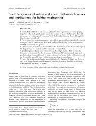
Van de Bogert et al.Benthic and pelagic metabolismof the lake, it is possible to partition metabolism between benthicand planktonic sources. Here “benthic” refers only to benthicprocesses occurring within the littoral zone (and thuswithin the mixed layer). In this analysis, we assume that theplanktonic GPP and R are uniform in space and benthic metabolismonly occurs where the bottom of the lake is within theupper mixed layer (>30% of the area of Peter Lake). To computeoxygen dynamics at any point x along a transect from shore tothe center of the lake, we adapt equation 3 as follows:Y = Y + ⎡m GPPb PAR(7)PAR− ⎤ 1 ⎡ GPPpRb txt , + xt , x⎢Δt ⎥ +1⎢ PAR − Rp t D Zt x t x t⎣ 24⎦ z PAR24Δ ⎤⎥ + + , ,x ⎣⎦As in the site-specific model, prediction errors Z x,tareautocorrelated and can be corrected for autocorrelationusing equation 6. Given a value of the spatial weightingfunction m x(explained below), measurements of PAR24 andPAR t, and estimates of D, equation 7 can be fitted to the datato estimate the parameters GPP b, R b, GPP p, and R pand theirconfidence intervals as described above for site-specificmetabolism.The value of m x(which is a function of distance from shore)can be viewed as the proportion of the GPP or R produced in1 m 2 of benthic habitat that is seen by a sensor at location x.A sensor directly above benthic sediment may “see” nearly allof the benthically derived metabolism produced there. A sensornear the boundary between the littoral and pelagic zonemay see only a portion of the benthically derived metabolismbecause the signal may be diluted by water mixing betweenthe zones. A sensor in the middle of the lake may see only asmall portion of the metabolic signal produced near shore (seeFig. 1). The sum of the benthic signal seen at all locations cannotbe more than the benthic area is capable of producing.Thus the mixing function is constrained by the area of benthicsediment in contact with the mixed layer. Two extreme, hypotheticalexamples illustrate this point. If there is no horizontalmixing of water, then 100% of the benthic signal would bemeasured in the littoral zone and 0% measured in the pelagic(Fig. 2a). On the other hand, if there were instantaneous mixing,the benthic signal would immediately be evenly spreadout through the entire epilimnion (Fig. 2b). Intermediate scenariosare more likely, and a couple of examples are drawn inFig. 2c. All of the intermediate scenarios can be described byan inverse tangent function transformed to have a rangebetween 0 and 1:m = ⎛−ax + π ⎞b(8)x ( )+⎝⎜⎠⎟ × 1tan 1 2 πThe shape of the function is determined by the parametersa (vertical stretch) and b (horizontal shift). Because the areaunder each curve is constrained by the area of the lake wherebenthic-littoral metabolism can occur, the two parameters (aand b) can be reduced to one unknown by setting the integralof the function (equation 9) from 0 to 1 equal to the ratio ofbenthic area to lake area (equation 10).1 ⎧⎪1 ⎡−112 ⎤∫ mxdx ( ) = ⋅⎨⋅ ⎢( ax + b)⋅ tan ( ax + b)− ln 1+ ( ax + b)(9)π a2( ) ⎥⎩⎪+ π ⋅ ⎫⎪x ⎬⎣⎦ 2 ⎭⎪Fig. 2. Idealized models of the mixing function used to distribute thebenthic metabolic signal along the transect. The x-axis is the ratio of thearea of the lake from shore to distance x to the area of the entire lake. A Bis the ratio of benthic-littoral area to lake area. The y-axis represents theproportion of benthic-littoral metabolism detectable at a point x. In a,there is no mixing and the entire oxygen signal from benthic metabolismremains in the littoral zone. In b, there is perfect mixing, and the oxygensignal from benthic processes is evenly spread along the entire transect.Examples of intermediate cases are shown in c. In each case, the areaunder the curve is equal to A B.149

Van de Bogert et al.Benthic and pelagic metabolism( )1A = m x dx = 1 ⋅ ⎧⎪1(10)a⋅ ⎡( a + b )⋅ −1( a + b )− 1+2 ⎤aB ∫ ( ) ⎢ tan ln 1 ( + ) ⎥π2+ π ⎫⎪⎨b ⎬0⎩⎪ ⎣⎦ 2 ⎭⎪1 ⎧⎪1 ⎡−11 ⎤⎫2 ⎪− ⋅⎨⋅ ⎢( b)⋅tan ( b)− ln( 1+b ) ⎥⎬π ⎩⎪ a ⎣2 ⎦⎭⎪The arbitrary parameter b can be expressed in terms of thevalue of m xat shore by setting x equal to 0 and solving equation8 for b.b= tan( m × π −π )(11)02During the fitting process, a single value of the intercept (m 0)is estimated for all sensor locations on a given day. Given anestimate of m 0and the ratio of benthic area to lake area, thevalue of b is calculated from equation 11 and the value of acan be solved numerically from equation 10 using the fzerofunction of Matlab 7.0, which finds the root of a continuousfunction of one variable.AssessmentSonde performance—We estimated 24-h GPP and R for each of5 days and for all 6 sondes placed at the same location in thecenter of Peter Lake. Between-sonde variability was low for alldays, and the pooled standard deviation between sondes was3.35 mmol m –2 d –1 , or about 9% of the average metabolism estimatesover the 5 days. In contrast, site-to-site variation in metabolismestimates when sondes were placed along transects was >3times this amount, with a standard deviation of 10.5 mmol m –2d –1 , or 38% of the average metabolism estimate over all transects.Site-specific estimates of metabolism—Using equation 3, weanalyzed 197 sonde-days to estimate GPP and R at each transectlocation. The model captured the diel pattern of dissolvedoxygen dynamics with only the processes of GPP, R, and diffusion(Fig. 3a). The autocorrelation term improved the fit ofthe model and resulted in nonautocorrelated residuals, but didnot change the estimates of the underlying processes (Fig. 3b).Estimates of metabolism for any given day varied based on thelocation of the measurement. For GPP, 40% of the days had acoefficient of variation (CV)

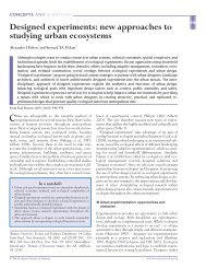
Van de Bogert et al.Benthic and pelagic metabolismFig. 4. Volumetric estimates of site-specific GPP (squares) and R (circles)with respect to distance from shore for 4 dates representative of the varyingspatial patterns observed (a–d). Error bars represent bootstrapped95% confidence intervals and may be obscured by the symbols.that are higher away from shore. We therefore applied thismodel to only the 15 transects in which metabolism decreasedfrom shore to the center of the lake. For 3 of these days, themodel could not adequately fit the diel oxygen curve becauseof irregularities in the shape of the curve that could not beexplained by our simple model. For the remaining 12 days,the simultaneously estimated oxygen curves fit as well ornearly as well as the fits for the individual sondes.Estimates of whole-lake GPP and R based on this modelwere higher than estimates based on single sondes in the middleof the lake. Over the 12 days analyzed, whole-lake GPPranged from 18.7 to 166 mmol O 2m –2 d –1 , with a mean of 54.0(Fig. 7a), whereas GPP estimated from a single sonde in themiddle of the lake had a mean of 37.3 mmol O 2m –2 d –1 , witha range of 8.82 to 134. Whole-lake R ranged from 17.9 to129 mmol O 2m –2 d –1 , with a mean of 52.5 (Fig. 7b). Estimatesof R based on a single sonde in the middle of the lake had amean of 34.6 mmol O 2m –2 d –1 , with a range of 6.20 to 92.2.The estimates for whole-lake GPP and R were highest from the3 transects we deployed in 2002 when the lake was fertilized.Modeled rates of pelagic metabolism were lower than measurementsof metabolism at the center of the lake: meanpelagic GPP was 32.2 mmol O 2m –2 d –1 and mean pelagic R was28.2 mmol O 2m –2 d –1 . Rates of benthic metabolism were morethan twice as high as pelagic metabolism when examined perunit area of littoral habitat, with mean benthic GPP and R of66.5 and 75.0 mmol O 2m –2 d –1 , respectively. When expressedin terms of whole-lake area, benthic GPP and R contributedslightly less (21.7 and 24.3 mmol O 2m –2 d –1 , respectively) toFig. 5. Metabolism values as a function of distance from shore for all 40days of samples on Peter Lake. Boxes represent middle 50% of the data,with the median shown as the center line. Circles show mean values andwhiskers extend to the most extreme value within 1.5 times the interquartilerange of the samples.whole-lake metabolism than pelagic processes. On average,benthic processes made up 39% of whole-lake GPP and 42% ofwhole-lake R but varied considerably between days (Fig. 7).Net ecosystem production also varied between habitats.Pelagic NEP (NEP p= GPP p– R p) was more often positive (netautotrophic), whereas benthic NEP was more often negative(net heterotrophic). Mean pelagic NEP was 4.10 mmol O 2m –2d –1 (range of –8.60 to 40.9), whereas mean benthic NEP was–2.61 (range of –21.4 to 10.3). Whole-lake NEP was on averageslightly positive, with a mean of 1.49 mmol O 2m –2 d –1 (rangeof –13.8 to 37.4).Wind as a homogenizing force—Between-site variation indaily metabolism estimates (GPP and R combined) wasinversely related to the average wind speed (r 2 = 0.33, P

Van de Bogert et al.Benthic and pelagic metabolismFig. 6. Comparison of metabolism values based on 3 different methods.Estimates from the center of the lake are shown in squares, estimatesbased on volume-weighted averages of all sensor locations are shown incircles, and spatially explicit whole-lake model estimates for the 12 dayswhen the model was run are shown with triangles. Estimates based onsingle, central sensors are often much lower than estimates whichaccount for spatial variability in metabolism.When average 5-min wind speeds topped 2.75 m s –1 for morethan a total of 1 of the first 18 h of a day (nearly half of alldays studied in 2003), standard deviation in daily metabolismestimates among sites was 5 mmol O 2m –2 d –1 and of these, 9 displayed the hypothesizedpattern of highest metabolism near shore and lowest atthe center of the lake (Fig. 8).DiscussionModels of dissolved oxygen at individual locations withina lake as well as simultaneous models of whole transectsrevealed that dynamics were not homogenous throughoutspace in our study lake. Indeed, severalfold differences inmetabolism estimates from site to site were common.Although these differences did not always follow predictableFig. 7. Estimates of whole-lake GPP and R (mmol O 2m –2 d –1 ) and thebenthic contribution of each based on the spatially explicit model. Errorbars show 95% confidence intervals based on 10,000 bootstrap iterations.Data from 2002 (fertilized) are shown using squares and data from2003 (not fertilized) are shown using circles.patterns, on average an estimate based on a single, centrallocation underestimated whole lake values.Epilimnetic water circulation may be one factor that determinesthe degree to which a single sonde estimate of metabolismadequately represents whole-lake metabolism. Water circulation(and the differential rates and patterns of that circulation throughtime) can mask the real heterogeneity in underlying ecosystemprocesses which occur at slower rates. When circulation occursquickly relative to the underlying biotic processes, measurementsof metabolism will be similar regardless of location, and a singlemeasurement location may provide a reliable estimate of wholelakeepilimnetic metabolism. When circulation occurs muchmore slowly relative to the biotic processes, site-to-site variationshould occur in a predictable manner, with highest values nearshore and lowest values in the center of the lake.As a driver of water circulation, measurements of wind speedcan provide one prediction of the degree of homogenizationin metabolism estimates among sites. When wind speeds arehigh, metabolism estimates are quite similar between locations.Even short periods of high wind are enough to set cir-152

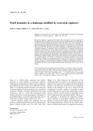
Van de Bogert et al.Benthic and pelagic metabolismFig. 8. Relationship between site-to-site variation in daily metabolismestimates (GPP and R combined) and the amount of time in the first 18 hof the day with 5-min average wind speeds greater than 2.75 m s –1 . Eachpoint corresponds to one 24-h transect from 2003. Filled-in points denotedays when metabolism was highest near shore and lowest in the centerof the lake and are the days when we were able to partition benthic andpelagic metabolism.culation patterns in motion that conceal the underlying heterogeneityin ecosystem processes. For Peter Lake, thereappeared to be a threshold of 1 h with 5-min average windspeeds above 2.75 m s –1 : above this threshold, metabolism estimateswere always similar among sites. This threshold is likelya function of the magnitude of the differences in underlyingecosystem processes. Larger differences between benthic andpelagic metabolism rates could raise this detection threshold.When wind speeds are low, other physical drivers (e.g., precipitation,convection currents) can provide homogenizingforces and may need to be considered.Differences among lakes (e.g., size, morphometry, andtrophic state) may also affect the degree to which a singlesonde estimate of metabolism adequately represents wholelakevalues (Fee 1979; Håkanson 2005). In large lakes withvery steep littoral zones (and thus small littoral area relativeto total lake area), pelagic metabolism may make up a largerproportion of the total. In this case, even if a sonde measuresnone of the benthic metabolism, the measurement should becloser to whole-lake values than one in a smaller lake withlarge littoral zones. The effect of lake size, however, is likelymore complicated and in need of further study. It is reasonableto hypothesize, for example, that across a gradient of increasinglake size, central sondes will receive less and less signalfrom the littoral zone because the increased distance allowsthe littoral signal to be muted by atmospheric diffusion. Thebalance between this signal loss and its initial magnitudewould likely determine how close a single estimate of metabolismin the center of lake approaches the true whole-lakevalue. In lakes smaller and shallower than Peter Lake, benthicmetabolism may make up a greater proportion of the total. Ifbenthic metabolism is not effectively measured by a centralsonde, the measurement may be a more extreme underestimateof the true whole-lake value. Alternatively, if the shorterdistance between the shore and center allows the benthic signalto reach the center of the lake without being muted byatmospheric diffusion, a single sensor may be able to accuratelymeasure whole system metabolism. In any given case,an investigator can use the approach presented here to examinespatial heterogeneity in metabolism and design a deploymentstrategy suitable for capturing whole-lake metabolism.In Peter Lake a sonde placed at a central location measuredpelagic metabolism and an unknown portion of benthic-littoralmetabolism. In the cases where we could apply the spatiallyexplicit model, we found that a sonde in the center of the lakemeasured only an average of 75% of the whole-lake epilimneticGPP and 73% of the whole-lake epilimnetic R. On these days,the central sonde only measured approximately 25% of thebenthic GPP and R—the remaining portion was not detectablewith a single sensor in the center of the lake. Because these dayshad the lowest rates of mixing as determined by wind speed,this estimate may be a lower bound on the proportion of benthicmetabolism seen by the central sonde.Ecologists often are more concerned with net ecosystemproduction than either GPP or R alone (Cole et al. 1994; 2000).The data presented here illustrate that NEP is also heterogeneouswith pelagic metabolism tending toward net autotrophyand benthic processes tending toward net heterotrophy.In this case, inference based on a single measurement maylead to erroneous conclusions about a lake’s trophic status.Similarly, Pace and Prairie (2005) report spatial variation inpCO 2within lakes and surmise that this variation is also dueto spatial heterogeneity in NEP.Although we were only able to apply the spatial model on 12of 40 days, the remainder of the deployments were still usefulfor measuring site-specific and volume-weighted epilimneticmetabolism. Furthermore, collecting data using automatedsamplers is fairly easy. There is not much difference in the workneeded to collect data for 3 days vs. 10 days because the additionalsampling costs only instrument time—not labor ormoney. What might be considered oversampling for answeringthe benthic-pelagic question is still useful for obtaining betterestimates of whole-lake metabolism. The benthic-littoral portioncan be inferred from days during the deployment whenweather conditions (e.g., low wind speed) allow the use of thespatially explicit model presented in this article.Comments and recommendationsThe results of this study suggest that ecologists interested inwhole-lake metabolism should recognize the potential for heterogeneityin within lake processes and acknowledge that singlesiteestimates may not represent whole-lake metabolism or153

Van de Bogert et al.Benthic and pelagic metabolismonly pelagic metabolism, but rather something between thesetwo endpoints. Determining whole-lake metabolism requiresan evaluation of the spatial heterogeneity in one’s study system:How large is the littoral zone—is it 1% or 50% of lakearea? How different are simultaneous metabolism estimatesfrom near shore and at the center of the lake? In larger lakes,are plankton patchy? Questions such as these should beaddressed over a period encompassing a representative rangeof weather patterns (e.g., wind, solar radiation, precipitation),and the answers will help investigators decide whether pursuingmeasurements at higher spatial resolution is necessary oruseful for their particular goals.Although the cost of sensors is dropping, it is still significant.Thus, more work is needed to determine the minimumnumber needed for accurate estimates of whole-lake metabolismacross systems. Our data show that on days with highwind speed, measurements are not significantly differentacross sites and therefore the only benefit of many sensors isto verify the uniformity of metabolism estimates. However,on days with low wind speeds, variation among sites may behigh or low and is not predictable with the data we collected.On low wind days, this study shows that for lakes similar toPeter Lake, the number of sensors needed is >1 and will likelyneed to include enough to separately sample the littoral zone,the pelagic zone, and perhaps a few places along the gradientbetween. Although Peter Lake is small, we suspect theseresults will be applicable for many lakes given that 97% of theworld’s lakes are smaller than or equal to the area of PeterLake and that lakes the same size or smaller account for 22%of the worldwide surface area of lakes (Downing et al. 2006).This study demonstrates the potential for in-lake heterogeneityto bias single-location estimates of whole-lake metabolismby underestimating benthic contributions. The degree towhich similar bias occurs in larger lakes is a question that stillneeds to be studied.Investigators interested in partitioning benthic and pelagicmetabolism from whole-lake values will need to employ severalsensors (4 to 6 were used in this study) along a littoralpelagicgradient. Although this study did not address the optimalnumber of sondes needed to answer this question, wenote that a minimum of 3 sensor locations is needed to be ableto simultaneously estimate the two end members of metabolismand the rate of mixing along the transect.The increased use of automated data acquired from sensorsalong with declining cost is leading to enhanced potential tomeasure ecosystem processes. Free-water oxygen measurementslike those used in this study overcome many of thelimitations of bottle and chamber methods, but there is stillmuch to learn about these methods, particularly what types ofsampling regimens are necessary to adequately capture ecosystemestimates of processes like metabolism. Without furtherevaluation of sensor-based methods, process estimates will sufferambiguities similar to traditional techniques. For example,just as traditional 14 C primary productivity methods measuresome unknown value between net and gross primary production(Peterson 1980), a single centrally located oxygen sensormay measure some unknown value between pelagic metabolismand whole-lake metabolism. These ambiguities may bereduced with improved sampling designs coupled with modelsthat incorporate spatial heterogeneity in ecosystem processes.ReferencesBade, D. L., and J. J. Cole. 2006. Impact of chemicallyenhanced diffusion on dissolved inorganic carbon stableisotopes in a fertilized lake. J. Geophys. Res. Oceans 111:C01014. [doi:10.1029/2004JC002684].Caraco, N. F., and J. J. Cole. 2002. Contrasting impacts of anative and alien macrophyte on dissolved oxygen in a largeriver. Ecol. Appl. 12:1496-1509.Carpenter, S. R., et al. 2005. Ecosystem subsidies: terrestrialsupport of aquatic food webs from C-13 addition to contrastinglakes. Ecology 86:2737-2750.Carpenter, S. R., and J. F. Kitchell. 1993. The Trophic Cascadein Lakes. London: Cambridge University Press.Chapra, S. C. 1997. Surface Water-Quality Modeling. New York:McGraw-Hill.Chen, C. C., J. E. Petersen, and W. M. Kemp. 2000. Nutrientuptakein experimental estuarine ecosystems: scaling andpartitioning rates. Mar. Ecol. Prog. Ser. 200:103-116.Cole, J. J., N. F. Caraco, G. W. Kling, and T. K. Kratz. 1994.Carbon-dioxide supersaturation in the surface waters oflakes. Science 265:1568-1570.Cole, J. J., and M. L. Pace. 1998. Hydrologic variability ofsmall, northern Michigan lakes measured by the additionof tracers. Ecosystems 1:310-320.Cole, J. J., M. L. Pace, S. R. Carpenter, and J. F. Kitchell. 2000.Persistence of net heterotrophy in lakes during nutrientaddition and food web manipulations. Limnol. Oceanogr.45:1718-1730.Downing, J. A., et al. 2006. The global abundance and size distributionof lakes, ponds, and impoundments. Limnol.Oceanogr. 51:2388-2397.Efron, B., and R. Tibshirani. 1993. An Introduction to theBootstrap. New York: Chapman & Hall.Fee, E. J. 1979. Relation between lake morphometry and primaryproductivity and its use in interpreting whole-lakeeutrophication experiments. Limnol. Oceanogr. 24:401-416.Fellows, C. S., H. M. Valett, and C. N. Dahm. 2001. Wholestreammetabolism in two montane streams: contributionof the hyporheic zone. Limnol. Oceanogr. 46:523-531.Gelda, R. K., and S. W. Effler. 2002. Metabolic rate estimatesfor a eutrophic lake from diel dissolved oxygen signals.Hydrobiologia 485:51-66.Gerhart, D. Z., and G. E. Likens. 1975. Enrichment experimentsfor determining nutrient limitation: 4 methods compared.Limnol. Oceanogr. 20:649-653.Håkanson, L. 2005. The importance of lake morphometry forthe structure and function of lakes. Int. Rev. Hydrobiol. 90:154

Van de Bogert et al.Benthic and pelagic metabolism433-461.Hanson, P. C., D. L. Bade, S. R. Carpenter, and T. K. Kratz. 2003.Lake metabolism: relationships with dissolved organic carbonand phosphorus. Limnol. Oceanogr. 48:1112-1119.Hartmann, D. L. 1994. Global Physical Climatology. SanDiego: Academic Press.Hilborn, R., and M. Mangel. 1997. The Ecological Detective:Confronting Models with Data. Princeton, N.J.: PrincetonUniversity Press.Iqbal, M. 1983. An Introduction to Solar Radiation. San Diego:Academic Press.Langdon, C. 1984. Dissolved oxygen monitoring system usinga pulsed electrode: design, performance, and evaluation.Deep-Sea Res. 31:1357-1367.Lauster, G. H., P. C. Hanson, and T. K. Kratz. 2006. Grossprimary production and respiration differences among littoraland pelagic habitats in northern Wisconsin lakes.Can. J. Fish. Aquat. Sci. 63:1130-1141.McCutchan, J. H., W. M. Lewis, and J. F. Saunders. 1998.Uncertainty in the estimation of stream metabolism fromopen-channel oxygen concentrations. J. N. Am. Benthol.Soc. 17:155-164.Mulholland, P. J., et al. 2001. Inter-biome comparison of factorscontrolling stream metabolism. Freshwater Biol. 46:1503-1517.Naegeli, M. W., and U. Uehlinger. 1997. Contribution of thehyporheic zone to ecosystem metabolism in a prealpinegravel-bed river. J. N. Am. Benthol. Soc. 16:794-804.Odum, H. T. 1956. Primary production in flowing waters.Limnol. Oceanogr. 1:102-117.Pace, M. L., and Y. T. Prairie. 2005. Respiration in lakes. In P. A.del Giorgio and P. J. L. Williams [eds.], Respiration in AquaticEcosystems. London: Oxford University Press, p. 103-121.Petersen, J. E., C. C. Chen, and W. M. Kemp. 1997. Scalingaquatic primary productivity: experiments under nutrientandlight-limited conditions. Ecology 78:2326-2338.Petersen, J. E., J. C. Cornwell, and W. M. Kemp. 1999. Implicitscaling in the design of experimental aquatic ecosystems.Oikos 85:3-18.Peterson, B. J. 1980. Aquatic primary productivity and the14C-CO 2method: a history of the productivity problem.Annu. Rev. Ecol. Syst. 11:359-385.Uehlinger, U., and M. W. Naegeli. 1998. Ecosystem metabolism,disturbance, and stability in a prealpine gravel bedriver. J. N. Am. Benthol. Soc. 17:165-178.United States Geological Survey. 1981a. New tables of dissolvedoxygen saturation values. Water Quality TechnicalMemorandum 81.11.———. 1981b. New tables of dissolved oxygen saturation values;amendment of quality of water technical memorandumno. 81.11. Water Quality Technical Memorandum81.15.Vadeboncoeur, Y., et al. 2003. From Greenland to green lakes:cultural eutrophication and the loss of benthic pathways inlakes. Limnol. Oceanogr. 48:1408-1418.Valentini, R., et al. 1996. Seasonal net carbon dioxideexchange of a beech forest with the atmosphere. Glob.Change Biol. 2:199-207.Wanninkhof, R. 1992. Relationship between wind-speed andgas-exchange over the ocean. J. Geophys. Res. Oceans97:7373-7382.Weiss, R. F. 1970. The solubility of nitrogen, oxygen, andargon in water and seawater. Deep Sea Res. 17:721-735.Submitted 1 September 2006Revised 22 February 2007Accepted 16 March 2007155