View - Departament de Matemàtica Aplicada II - UPC

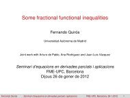
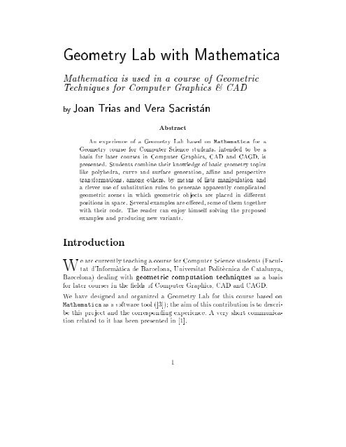
Geometry Lab with MathematicaMathematica isusedinacourse of GeometricTechniques for Computer Graphics & CADby Joan Trias and Vera SacristanAbstractAn experience of a Geometry Lab based on Mathematica for aGeometry course for Computer Science students, intended to be abasis for later courses in Computer Graphics, CAD and CAGD, ispresented. Students combine their knowledge of basic geometry topicslike polyhedra, curve and surface generation, ane and perspectivetransformations, among others, by means of lists manipulation anda clever use of substitution rules to generate apparently complicatedgeometric scenes in which geometric objects are placed in dierentpositions in space. Several examples are oered, some of them togetherwith their code. The reader can enjoy himself solving the proposedexamples and producing new variants.IntroductionWe are currently teaching a course for Computer Science students (Facultatd'Informatica de Barcelona, Universitat Politecnica de Catalunya,Barcelona) dealing with geometric computation techniques as a basisfor later courses in the elds of Computer Graphics, CAD and CAGD.We have designed and organized a Geometry Lab for this course based onMathematica as a software tool ([3]) the aim of this contribution is to describethis project and the corresponding experience. A very short communicationrelated to it has been presented in [1].1

Describing the experienceThe course is intended to cover dierent topics that are useful for computergraphics and computer aided design among others, some of them are: polyhedra,generation of curves and surfaces, ane bi- and three-dimensionaltransformations, perpective transformations, elementary methods of curveand surface design in CAD, geometric algorithms. During the course ourstudents must and also achieve whatwe could consider a certain maturityinthree-dimensional geometry as well as in geometric objects manipulation.More than presenting a classical course covering these subjects, we havepreferred to teach students the basic geometric operations they will needwhile developing geometric applications in computer graphics and relatedelds. We have identied some of these operations namely we want ourstudents to be able to perform the following ones: Place geometric 3D objects onto a plane, such as in gure 1.Figure 1. Torus generatedby shapes that has been putin tangent position onto theplane x + y + z ; 3=0. Draw 2D objects (curves, polygons or similar) onto a plane, for exampleonto the faces of some regular polyhedron (as can be seen in gure 2). Construct geometric objects that are in some sense dened by an \axis"or at least the position of which in space can be essentially determinedby the position of an axis, as would be for example in the case of a cylinder,a cone, an helicoid o a torus (the axis we can consider in the lastcase being the normal to the diametral plane, the problem illustrated2

Figure 2. Rhodonea, epitrochoids and other classical \mechanical"or \spirographical" curves that have been put on severalfaces of a dodecahedron generated byPolyhedra.in gure 1 can be reformulated in terms of an \axis" problem). Figure3 shows an example of this kind of problem.Figure 3. Constructing a circular helix around an axis determinedby the origin and the point (1 1 1).Another problem related to that one could consist of constructing acircle with its center in a curve and placed onto the plane perpendicularto the curve at that point. This can be a point of departure for thesynthesis of tubular surfaces. Produce the most common ane transformations although many problemscan be solved directly by changing the coordinate systems, studentsmust know the specic language of transformations and use it tosolve geometric problems, as for example in gure 4.3

Figure 4. A cylinder in original positionhas been transformed to produceanother copy of it with an axisnow determined by the baricenters ofthe two missing faces of the dodecahedron.As can be seen, our course has a highly practical orientation, that makesnecessary a strong activity in a geometry lab. The examples we have seenare typical exercices we propose to our students.The main toolsWe distinguish between geometric and programming tools.a) Geometric toolsFrom the point ofviewofmathematics, and specically of geometry,therequired background is not much extensive the main tool we sistematicallyuse is the coordinate transformation, specially between cartesian coordinatesystems.To establish some notation, recall that if we consider two coordinate systems,S =(O f~e 1 ~e n g), with O being the origin and f~e 1 ~e n g the basisof the corresponding vector space, determining the coordinate axes, and a\new" coordinate system given by S 0 =(O 0 f~e 10 ~en 0 g), then the \old"coordinates X of a point, and the \new" ones X 0 of the same point arerelated, as is well known, by the matrix equationX = AX 0 + Wwhere W (S)= ;;! OO 0 is the position vector of the new origin expressed in thesystem S, and A is the \change of basis matrix", formed with the columnvectors of the new basis as linear combinations of the old one here W ,4

X and X 0 are also column vectors. We can also derive the relation X 0 =A ;1 (X ; W ). We shall refer to this transformation as the \inverse" one,while the former version will be called the \direct" one.Students can program constructions of complex three-dimensional sceneswith a sistematic and clever use of coordinate transformations, making aproper choice of the coordinate systems involved, sometimes concatenatingand sometimes combining direct and inverse changes. A typical example ofuse of direct and inverse transformations can be seen in gure 5, correspondingto a variant of one of the exercices our students must solve. Seeminglycomplicated efects are not dicult to generate.Figure 5. Observethe cardioid with aninner one, both tangentat a commonpoint.Our main tool is very simple, and with such a simple tool we are able to govery far, from the point of view of the complexity of geometric scenes ourstudents are able to produce.b) Programming toolsFrom the point ofviewof programming, there are many reasons thatexplain why we use Mathematica let us mention, among others, the followingones:5

Proximity to mathematical language, particularly matrix and vectorcalculations, with a simple notation. Extensive supply of geometric objects, as well as incorporated functionsto produce geometric objects such ascurves or surfaces. Powerful 3D graphics processing. Powerful manipulation of lists. Powerful and precise substitution rules.Let us discuss in the sequel the before mentioned items.Proximity to mathematical language allows us to write Mathematica functionsalmost as if we were writing mathematical functions or expressionsconsider for example the denition of norm derived from the dot product:norm[v_]:=N[Sqrt[v.v]]or the denition of cross product:e1={1,0,0}e2={0,1,0}e3={0,0,1}vectorProduct[u_,v_]:=N[{Det[{u,v,e1}],Det[{u,v,e2}],Det[{u,v,e3}]}]The richness of geometric objects, ranging from the most elementary ones(geometric primitives like Polygon, Line, Point, and others) to more complexones, allows us to generate non trivial objects. We also makeaheavy useof the packages Shapes and Polyhedra and, to a minor extent, of Surface-OfRevolution,aswell as of the incorporated functions to produce curves orsurfaces.Powerful 3D graphics processing is important because it allows our studentsto concentrate on geometry, which is the objective of the course: once theplan to solve a problem is traced from the point of view of geometry, then6

Mathematica does the rest, specially 3D rendering and perspective projections,so that they don't need to pay attention to such details, important, butlengthy to solve.Powerful manipulation of lists allows to easily manipulate geometric structures,due to the list structured coding of geometric objects and scenes thepossibility of coding complex geometric scenes by means of lists renders easytheir manipulation and transformation, and permits cumulative constructionfrom simple to more complex structures.As an example, load the package shapes (and suppose it loaded from nowon) and generate a cylinder cyl0 withNeeds["Graphics`Shapes`"]cyl0=Cylinder[]Show[Graphics3D[cyl0]]Observe that what wehave really obtained is a list of polygons, which are thequadrangular faces of the lateral surface by means of which we approximatethe true cylinder by a polyhedral surface indeed, we have cyl0 equal to{Polygon[{{0.951056516295153, 0.3090169943749474, 1},...{0.809016994374947, 0.5877852522924732, 1}}],...Polygon[{{1., 0, 1}, {1., 0, -1},{0.951056516295153, 0.3090169943749474, -1},{0.951056516295153, 0.3090169943749474, 1}}]}It is not dicult now to manipulate this structure having in mind that manipulatinglists produces geometric manipulation of the scenes (gure 6):cyl00=Drop[cyl0,{2,5}]Show[Graphics3D[cyl00],Boxed->False,ViewPoint->{2,2,2}]Perhaps one of the most important characteristics of Mathematica forusisthe possibility to easily program selective substitutions inside a complicated7

Figure 6tree-like structure describing a geometric object or a geometric scene thisallows us to easily program transformations and in general manipulations ofgeometric objects, changing only the coordinates, but retaining the overallstructure.Let us consider an example suppose we want to transform the cylinder cyl0by (x y z) 7! (2x 3y z) just write a substitution rule and look at the resultby representing both objects in the same scene (gure 7):cyl1=cyl0/.{x_?NumberQ,y_?NumberQ,z_?NumberQ}->{2x,3y,z}Show[Graphics3D[{cyl0,cyl1}]]Now we could apply a new transformation to the scene scene={cyl1,cyl0},such as for example to interchange the roles of the axes z and x it sucesto use a substitution rule (see the result in gure 7).scene2=scene/.{x_?NumberQ,y_?NumberQ,z_?NumberQ}->{z,y,x}Show[Graphics3D[scene2]]Figure 7With these possibilities of substitution rules, the point transformation X =AX 0 + W can be easily enlarged to produce the transformation of a wholegeometric object or even a complete geometric scene formed byseveralobjects (with a slightly more robust formulation even graphic objects can betransformed) this means that a complex object or scene can be expressed,as a whole, in an another coordinate system, with no need of decomposingor taking apart the elementary geometric components of the complex object,express each of them in the old or new coordinate system, and nally reconstructthe whole structure, as had to be done in a more classic programming8

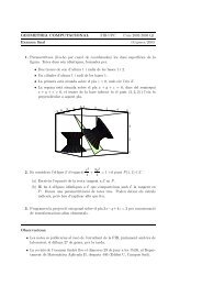
environment. That is the point that makes this method so powerful and easyat the same time, in order to perform geometric transformations.The most simple version for a function transforming new coordinates intoold ones could be the following one, in the 3D case:coordinateTransf[(*X=AX'+W*)obj_, (*object or scene*)A_, (*change of basis (row) matrix*)W_ (*new origin*)]:=N[obj]/.{a_?NumberQ,b_?NumberQ,c_?NumberQ}->A.{a,b,c}+WThis function can be trivially completed to cope with the \inverse" coordinatetransformation, in the case where both vector bases are orthonormal, andeven in other cases, and also enhanced from the programming point ofviewfor the sake of simplicity, we express it in this form.With these tools in hand we are able to challenge our students with sosticated(and, we expect, imaginative) 3D geometric scenes.Letuspresentnow the general strategy of resolution of geometric problemsconsisting of scenes or objects we wish to produce using coordinate transformations,by means of the resolution of some examples.A basic exampleLet us begin with a simple problem: drop a circular cylinder cylA of radius 1,height 1,onto the plane : x + y + z = 3 such that the cylinder's axis passesthrough the point P =(1 1 1) 2 . First of all, generate such a cylinder incanonical position, that is with its symmetry axis coincident with coordinateaxis Oz and the base onto the plane z =0:cylA=ParametricPlot3D[{Cos[t],Sin[t],z},{t,0,2Pi},{z,0,1},PlotPoints->{20,2},DisplayFunction->Identity][[1]]This will be a 3D object precomputed once and for all we thus obtain thecoding not only of this cylinder but of all the cylinders with the same metriccharacteristics in any other cartesian system of coordinates (O 0 fx 0 y 0 z 0 g),9

provided that its position mimics exactly the position of the canonical one,that is, its axis coincides with the third axis of coordinates O 0 z 0 and its baseis on the coordinate plane z 0 =0. This is the basic idea for our strategyof resolution of this kind of problems: suppose the problem solved and thecylinder put onto the plane in the right position place an appropiate cartesiansystem of coordinates, related to the plane and to the cylinder: thenthe description of the object on top of the plane expressed in this system ofcoordinates is exactly the canonical one hence it only remains to express itin the old cartesian system. So, the only problem is to construct the newcartesian system so that the third axis O 0 z 0 coincides with the axis of thecylinder and such that z 0 = 0 is identied with the plane .Let us construct such a basis manually (it can be automatized):uu3={1,1,1} (*normal to the plane*)u3=uu3/norm[uu3]uu1=vectorProduct[u3,e3] (*for example, if not dependent*)u1=uu1/norm[uu1]u2=vectorProduct[u3,u1]AA={u1,u2,u3}A=Transpose[AA]Now, with W={1,1,1}, we can consider the new coordinate system andexpress the cylinder in the ancient one:plane=Polygon[{{3,0,0},{0,3,0},{0,0,3}}]axes[length_:1]:={Line[{{0,0,0},{length,0,0}}],Line[{{0,0,0},{0,length,0}}],Line[{{0,0,0},{0,0,length}}]}axesOnThePlane=coordinateTransf[axes[],A,W]cylinderOnThePlane=coordinateTransf[cylA,A,W]Show[Graphics3D[{axes[3.2],plane,axesOnThePlane}],Boxed->False]Show[Graphics3D[{axes[3.2],plane,cylinderOnThePlane}],Boxed->False]and see the result in gure 8.10

Figure 8A more complete exampleLetusnow consider a more complex scene (gure 9), composed by part of acylinder generated by shapes, of radius 2, height 8, with axis coincident withOy, an icosahedron obtained with Polyhedra, reescaled and with center at(3:5 ;1 2:5) (by means of a coordinate transformation) and three spheresobtained with shapes with centers, respectively, at(0 0 0), (;3 0 0) and(0 0 3), that are \looking at" a point, the center of the polyhedron, that is,with their polar axes pointing to that point.Figure 9This can be obtained by the following code (where we have slightly automa-11

tized the process of contructing an orthonormal basis, in which the third axisis given by two points supposed to be dierent and is also supposed not tobe parallel to the Oz axis):Needs["Graphics`Polyhedra`"]basis[A_,B_]:=Module[{uu3,uu1},uu3=B-A (*supposed different*)u3=uu3/norm[uu3]uu1=vectorProduct[u3,e3] (*supposed independent*)u1=uu1/norm[uu1]u2=vectorProduct[u3,u1]Transpose[{u1,u2,u3}]]lookAt={3.5,-1,2.5}icosa0=Icosahedron[]scale={{.3,0,0},{0,.3,0},{0,0,.3}}icosa1=coordinateTransf[icosa0,scale,lookAt]cyl0=Cylinder[2,4,30]cyl1=Drop[cyl0,{2,5}]cyl2=cyl1/.{x_?NumberQ,y_?NumberQ,z_?NumberQ}->{x,z,y}sph0=Sphere[1,20,20]center1={0,0,0}sph1=coordinateTransf[sph0,basis[center1,lookAt],center1]L1=Line[{center1,lookAt}]center2={0,-3,0}sph2=coordinateTransf[sph0,basis[center2,lookAt],center2]L2=Line[{center2,lookAt}]center3={0,3,0}sph3=coordinateTransf[sph0,basis[center3,lookAt],center3]L3=Line[{center3,lookAt}]12

Show[Graphics3D[{{GrayLevel[.7],cyl2},{GrayLevel[1],sph1,sph2,sph3,icosa1},{L1,L2,L3}}], Boxed->False, PlotRange->All, Lighting->False]Now we are ready to place the new object just created into any other scene,in any desired position (as onto a plane, like in gure 10).Figure 10Some other examplesThere are many additional programming exercices we propose to our studentsthe complete set of them for our Geometry Lab can be found in [2].Let us mention only a sample of them.We sistematically use ParametricPlot and ParametricPlot3D to generatecurves and surfaces, usually in general position in space consider for examplegure 11.Concerning 2D ane transformations, an exercise incorporating a great numberofdierenttransformations is the construction of a toothed wheel fromthe description of its smallest piece: the tooth. After the programming task,prisms based on the wheel can be generated and used as a component inmore complex scenes, concerning now 3D ane transformations, such asfor13

Figure 11. Constructing a spiral helix, with plane projectiononto an Archimedes spiral, and then putting it in a precise positiononto the plane x + y + z =3.example specular symmetry (see gure 12).Figure 12. Toothed wheels, prisms and specular symmetry.Another interesting exercise is the generation of polyhedra of revolutionfrom a plane polygonal prole, as a standard tool for volume generationin solid modelling and CAD one of the most popular objects is the chessqueen, that we also integrate in more complex geometric compositions, suchas in gure 13.14

Figure 13. Compositionwith chess piecesof revolution.ConclusionsOur geometry lab is not merely an experimental complement in our course,but it is an integral part of it, and one of the most important ones. Withoutthe possibilityofusingMathematica wewould not have been able to organizethe course as we have done, and without it our course would have been verydierent.Our impression is that students learn much better geometry with such kindof lab exercices, they become enthousiastic about them and they realize theimportance of the relationship between theory and applications.With our experience, we hope wehavecontributed to makemany people morefamiliar with mathematics laboratories, specially geometry ones, and to behelping that way to the incorporation of the new developing technologiesin mathematical education, to put the teaching of mathematics in a newhigh-tech environment, and consequently, on a new and modern basis.As a byproduct of our preparation of materials for the course we have atour disposal an extensive set of Mathematica functions that constitute apowerful tool for mathematical calculation and illustration (specically, inthe dicult eld of 3D geometrical illustration) once it will be organized asa Mathematica package, it will become available. By now, our contributionto this use of Mathematica in preparing graphic material for teaching canbe found in [2]. Some other authors in our Department have developed15

Mathematica packages for geometrical calculation and have used them as anillustration tool for educational purposes to prepare classroom material ([4]).References[1] Hurtado, F., Trias, J.: Tecnicas geometricas para la informatica graca:practicas de laboratorio, Actas de las Jornadas sobre Nuevas Tecnologasen la Ense~nanza de las Matematicas en la Universidad (Eds. A.Montes,J.M.Brunat), TEMU-95, (241-250), Departament de Matematica AplicadaII, Universitat Politecnica de Catalunya, 1995.[2] Trias, J.: Geometria Computacional, practiques de laboratori, UniversitatPolitecnica de Catalunya, 1995.[3] Wolfram, S.: Mathematica, a system for doing mathematics by computer,Addison-Wesley, 1991.[4] Xambo, S., Grane, J.: Geometra con Mathematica, Actas de las Jornadassobre Nuevas Tecnologas en la Ense~nanza de las Matematicasen la Universidad (Eds. A.Montes, J.M.Brunat), TEMU-95, (425-457),Departament de Matematica Aplicada II, Universitat Politecnica de Catalunya,1995.About the authorsBoth authors are mathematicians and Professors of Mathematics in the Departamentde Matematica Aplicada II, Universitat Politecnica de Catalunya,Barcelona, and are teaching courses in Computational Geometry.Their research interest is also centered in the eld of Discrete, Combinatorialand Computational Geometry (complexity theory and algorithm design).16

Both are enthousiastic about the use of advanced mathematical software forclassroom laboratories, as a valuable aid in teaching mathematics.Joan TriasDept. de Matematica Aplicada IIFacultat d'Informatica de BarcelonaPau Gargallo, 5Universitat Politecnica de CatalunyaE-08028 Barcelona, Spaine-mail: avtrias@ma2.upc.esVera SacristanDept. de Matematica Aplicada IIFacultat d'Informatica de BarcelonaPau Gargallo, 5Universitat Politecnica de CatalunyaE-08028 Barcelona, Spaine-mail: vera@ma2.upc.es17