Digital Signal Processing Chapter 7: Parametric Spectrum Estimation
Digital Signal Processing Chapter 7: Parametric Spectrum Estimation
Digital Signal Processing Chapter 7: Parametric Spectrum Estimation

Create successful ePaper yourself
Turn your PDF publications into a flip-book with our unique Google optimized e-Paper software.
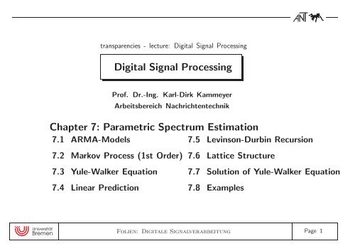
transparencies - lecture: <strong>Digital</strong> <strong>Signal</strong> <strong>Processing</strong><strong>Digital</strong> <strong>Signal</strong> <strong>Processing</strong>Prof. Dr.-Ing. Karl-Dirk KammeyerArbeitsbereich Nachrichtentechnik<strong>Chapter</strong> 7: <strong>Parametric</strong> <strong>Spectrum</strong> <strong>Estimation</strong>7.1 ARMA-Models 7.5 Levinson-Durbin Recursion7.2 Markov Process (1st Order) 7.6 Lattice Structure7.3 Yule-Walker Equation 7.7 Solution of Yule-Walker Equation7.4 Linear Prediction 7.8 ExamplesFolien: <strong>Digital</strong>e <strong>Signal</strong>verarbeitung Page 1
7.1 ARMA-Models7. <strong>Parametric</strong> <strong>Spectrum</strong> <strong>Estimation</strong>H AR (z) = 1A(z) = 1∑1 + n a ν z −νν=1H MA (z) = B(z) = 1 +m∑b µ z −µµ=1∑H ARMA (z) = B(z)1 + m b µ z −µA(z) = µ=1∑1 + n a ν z −νν=1<strong>Parametric</strong> <strong>Spectrum</strong> <strong>Estimation</strong> Page 2
7.2 Markov Process as an Example for a 1st Order AR-Modelx(k) = q(k) − a 1 · x(k − 1) ⇒ H(z) =11+a 1 z −1a 1 = −0.5a 1 = +0.5r xx (κ) →1.510.50-0.5a) Beispiel 1: AKF-1-10 -5 0 5 10κ →S xx (e jΩ ) →b) Beispiel 1: LDS43.532.521.510.50-1 -0.5 0 0.5 1Ω/π →e) Beispiel 3: komplexe AKFa 1 = −0.5e jπ/2 o ˆ= Re{r xx }10.5x ˆ= Im{r xx }0-0.5-1-10 -5 0 5 10r xx (κ) →1.5κ →S xx (e jΩ ) →4r xx (κ) →1.510.50-0.5c) Beispiel 2: AKF-1-10 -5 0 5 10κ →f) Beispiel 3: unsymm. LDS3.532.521.510.50-1 -0.5 0 0.5 1Ω/π →S xx (e jΩ ) →d) Beispiel 2: LDS43.532.521.510.50-1 -0.5 0 0.5 1Ω/π →• limited by model order!• for a 1 ∈ IR ⇒ onlylow- or highpassprocesses producibleMarkov Process Page 3
7.4.1 Linear Prediction: Derivation of the Wiener-Hopf-EquationFrom a sample fuction x(k) of a stationary, mean-free process X(k) an estimate ˆx(k)shall be computed based on past values of x(k) .^( x k)x( k) z –1 P( z)e( k)–+Pe ( z )A prediction-filter P(z) is excited by x(k − 1) ; e(k) is the prediction error.The prediction-error-filter is defined bySample function of the prediction errorP(z) = ∑ nν=1 p ν · z −ν+1 , p ν ǫ CP e (z) = 1 − z −1 · P(z) = 1 − ∑ nν=1 p ν · z −ν .e(k) = x(k) − ∑ nν=1 p νx(k − ν)Linear Prediction Page 4
Past values x(k − 1), · · · ,x(k − n) are summarized in a vector⎡ ⎤x(k − 1)x(k − x(k − 2)) =⎢⎣. ⎥⎦x(k − n)For the coefficients of the predictor definitions of vectors are⎡ ⎤ ⎡ ⎤p 1 p ∗ 1p 2p ∗ 2p =; ¯p =⇒ ¯p H = [p⎢⎣. ⎥ ⎢⎦ ⎣. ⎥1 , p 2 , · · · , p n ]⎦p np ∗ nWith the above definitions we can rewrite the convolution as a scalarproducte(k) = x(k) − ¯p H x(k − ) ;e ∗ (k) = x ∗ (k) − x H (k − )¯pLinear Prediction Page 5
Wiener-Approach for solving the problem of prediction:e(k) → E(k) x(k) → X(k)E{|E(k)| 2 } = E{E(k) · E ∗ (k)} = ! Min.E{|E(k)| 2 } = E{(X(k) − ¯p H X(k − ))(X ∗ (k) − X H (k − )¯p)}= E{X(k) · X ∗ (k)} − ¯p H E{X(k − ) · X ∗ (k)}− E{X(k) · X H (k − )}¯p+¯p H E{X(k − ) · X H (k − )}¯p (1)It is E{X(k)·X ∗ (k)} = σX 2 and furthermore E{X(k− )·X H (k − )} = △ ¯R XX the autocorrelationmatrixwith conjugate complex elements.With the definition of the autocorrelation-vector we obtain:¯r XX = E{X ∗ (k)X(k − )} = [rXX(1), ∗ ...,rXX(n)] ∗ T⇒ E{|E(k)| 2 } = ¯p H ¯R XX¯p − ¯p H¯r XX −¯r H XX¯p + σX 2 .Linear Prediction Page 6
Conjugating all elements yields inIntroducing the quadratic extensionE{|E(k)| 2 } = p H R XX p − p H r XX − r H XXp + σ 2 X .E{|E(k)| 2 } = (p H R XX − r H XX)R −1XX(R XX p − r XX ) − r H XXR −1XXr XX + σ 2 XThe global minimum can be found by setting the term containing p equal to zero. IfR XXis non-singular (in general fulfilled for autocorrelation-matrices) we can set thefollowing linear equation as the condition for a minimum of the prediciton-error :R XX p − r XX = 0.This results in the Wiener-Hopf-Equation providing the coefficient vector.p = R −1XXr XX .• The solution for the nonrecursive prediction-filter is given by the inversionof the autocorrelation-matrix.Linear Prediction Page 7
The power of the remaining prediction-error isMin{E{|E(k)| 2 }} = σ 2 X − rH XXR −1XXr XX .Rewriting the equation using the coefficient-vector p results inMin{E{|E(k)| 2 }} = σ 2 X − rH XXp.Linear Prediction Page 8
7.4.2 The Principle of OrthogonalityExamining the conjugate crosscorrelation-vector⎧⎡⎪⎨¯r EX = E{E ∗ (k) · X(k − )} = E⎢⎣⎪⎩and recalling thatE ∗ (k) · X(k − 1)E ∗ (k) · X(k − 2).E ∗ (k) · X(k − n)⎤⎫⎪⎬⎥⎦⎪⎭e(k) = x(k) − ¯p H x(k − ) ; e ∗ (k) = x ∗ (k) − x H (k − )¯p⇒ ¯r EX = E{[ X ∗ (k) − X H (k − ) ¯p ] · X(k − )}⇒ ¯r EX = E{X(k − ) · X ∗ (k)} − E{X(k − ) · X H (k − )} · ¯pExpressing the expectation values by the help of the autocorrelation-vector and -matrixwith further conjugation givesr EX = r XX − R XX p .Linear Prediction Page 9
For p we insert the solution of the Wiener-Hopf-Equation and since the crosscorrelationvectorvanishesThe principle of orthogonality is:r EX = r XX − R XX [R −1XXr XX ] = 0• The prediction-error-process E(k) and the past values of the processX(k − 1),...,X(k − n) are orthogonal to each other.The ’gapped function’ for a predictor of order n is defined asg n (κ) = E{E(k) · X ∗ (k − κ)}.Since r EX = r XX − R XX [R −1XXr XX ] = 0 the gapped function has the propertyg n (κ) = 0 , 1 ≤ κ ≤ n ;Linear Prediction Page 10
7.4 Linear Prediction (Overview)approach: E{|E(k)| 2 } = min; → σE 2 = σ2 X − rH XX R−1 XX r XXsolution: p = R −1XX · r XX using R XX = E{XX ∗ },and r H XX = [r∗ XX (1), · · ·,r∗ XX (n)]orthogon.: E{E ∗ (k)[X(k − 1), · · · ,X(k − n)] T } = 0gappedfunction:relationship between the linear prediction and the Yule-Walker-equation:a = −R −1XX · r XX→ σ 2 Q · |Pe(ej Ω )| 2|A(e j Ω )| 2= σ 2 QLinear Prediction Page 11
Prediction of Bandlimited White NoiseS VV (jω)A bandlimited white noise process V (k) sampled atf A = 1/T has the ACFN 02−ω gω gωr V V (κT) = σ 2 V · sin(ω gTκ)ω g Tκ , with σ2 V = f g · N 0 .For a first order predictor we getp 1 = r V V (T)r V V (0) = sin(ω gT)ω g Tand σ 2 E = σ2 V − r V V (T) · rV V (T)r V V (0) .60a) PrädiktionsgewinnG/dB →504030n=1620n=210n=100 0.2 0.4 0.6 0.8 1Ω g /π →The prediction gain G dB then is( ) σ2G dB = 10log V10G dB = 10log 10[(1 −σ 2 E(sin(ωg T)ω g T) 2)] −1Linear Prediction Page 12
7.5 Levinson-Durbin Recursion∑A r (z) = r a r,ν · z −ν → iterat. increment of order → A r+1 (z) = r+1 ∑a r+1,ν · z −νν=0design of the gapped function r + 1: g r (κ) = 0 for 1 ≤ κ ≤ rg r (r + 1 − κ) = 0g r (κ) − γ r+1 · g ∗ r(r + 1 − κ)→ g r (r + 1) − γ r+1 · g ∗ r(0)ν=0for 1 ≤ κ ≤ r!= 0 for 1 ≤ κ ≤ r + 1!= 0 → γ r+1 = g r(r + 1)gr(0)∗r + 1: → g r+1 (κ) = g r (κ) − γ r+1 · g ∗ r(r + 1 − κ)PARCOR-coefficients (PARtial CORrelation):γ r+1 =g r (κ) = E{X ∗ (k − κ) · E r (k)} = r ∑ν=0r∑ν=0a r,ν r XX (r+1−ν)r∑ν=0a ∗ r,ν r XX(ν)whereby:a r,ν E{X(k − ν)X ∗ (k − κ)}} {{ } ; }{{} = r XX(κ − ν)Levinson-Durbin Recursion Page 13
ecursive calculation of the prediction errors powerr∑r∑g r (0) = a}{{} r,0 ·r XX (0)+ a r,ν ·r XX (−ν) = σX+2 a r,ν rXX(ν) ∗ = σX 2 +r H XX · }{{} a=1ν=1ν=1−R −1XXr XXWiener-Hopf solution: min { E{|E(k)| 2 } } = σ 2 E = σ2 X −rH XX R−1 XX r XX;recursion: g r+1 (0) = σr+1 2 = g r (0) − γ r+1 gr(r ∗ + 1)} {{ } = σ2 r − γ r+1 gr(r ∗ + 1)using the definition γ r+1 = g r(r+1)g}{{} r(0)∗ → σr 2 γ r+1 = g r (r + 1)σr2σ 2 r+1 = σ 2 r − γ r+1 · γ ∗ r+1 σ 2 r → σ 2 r+1 = σ 2 r[1 − |γ r+1 | 2 ] thus:• |γ r+1 | < 1, because the power must be σ 2 r+1 > 0• σ 2 r+1 ≤ σ 2 r• limr → ∞r > nγ r = 0; σ 2 r+1 → σ 2 r → σ 2 Q if X(k) nth order AR-modelg r (0) = σ 2 E =: σ2 rLevinson-Durbin Recursion Page 14
ecursion for the predictive coefficients (Levinson-Durbin recursion)into the recursion for the “Gapped Function”: g r+1 (κ) = g r (κ) − γ r+1 · gr(r ∗ + 1 − κ)∑insert the definition g r (κ) = r a r,ν r XX (κ − ν) :∑r+1ν=0a r+1,ν r XX (κ − ν) =ν=0r∑a r,ν r XX (κ − ν) − γ r+1 ·ν=0r∑a ∗ r,ν rXX(r ∗ + 1 − κ − ν) ∗)convert the right side: (second term substitute r + 1 − ν = µ)r∑γ r+1 a ∗ r+1 ∑r,ν r XX (κ − (r + 1 − ν)) = γ r+1 a ∗ r,r+1−µ r XX (κ − µ)ν=0µ=1r∑entirely ∗) : a r,0 r XX (κ) + a r,ν r XX (κ − ν)r∑ ν=1− γ r+1 a ∗ r,r+1−µ r XX (κ − µ) − γ r+1 a ∗ r,0 r XX (κ − (r + 1))µ=1= r XX (κ) −γ} {{ } r+1 r XX (κ − (r + 1)) +a r,0 = 1ν=0r∑[(a r,ν − γ r+1 · a ∗ r,r+1−ν) · r XX (κ − ν)]ν=1Levinson-Durbin Recursion Page 15
comparison of the coefficients left and right of ∗) (left side: separation of 2 terms):∑r+1ν=0r∑a r+1,ν r XX (κ − ν) = r XX (κ) + a r+1,r+1 r XX (κ − (r + 1)) + a r+1,ν r XX (κ − ν)= r XX (κ)−γ r+1 r XX (κ − (r + 1)) +ν=1r∑[a r,ν − γ r+1 · a ∗ r,r+1−ν] · r XX (κ − ν)ν=1a r+1,ν = a r,ν − γ r+1 · a ∗ r,r+1−ν(for ν = 1 ,...,r)a r+1,r+1 = −γ r+1vectorized expression:⎡ ⎤ ⎡1 1a r+1,1a r+1,2.=.⎢⎣ a r+1,r⎥ ⎢⎦ ⎣a r+1,r+1 0a r,1a r,2a r,r⎤⎥⎦⎡− γ r+1 ⎢⎣0a ∗ r,ra ∗ r,r−1.a ∗ r,11⎤⎥⎦Levinson-Durbin Recursion Page 16
Levinson-Durbin Recursion• initialization (r = 0): a 0,0 = 1σ0 2 = r XX (0)• 1st iteration (r = 1) :γ 1 = r XX (1)/r XX (0)[ ] [ ] [ ]1 1 0= − γ 1a 11 0 1→ a 11 = −γ 1σ 2 1 = [1 − |γ 1 | 2 ] · σ 2 0 .• rth iteration (r = 2, ...,n) :γ r =r−1 ∑ν=0a r−1,ν r XX (r − ν)σ 2 r−1Levinson-Durbin Recursion Page 17
⎡⎢⎣⎤1a r,1.⎥⎦a r,r=⎡⎢⎣1a r−1,1.a r−1,r−10⎤⎥⎦⎡− γ r ⎢⎣0a ∗ r−1,r−1.a ∗ r−1,11⎤⎥⎦σr 2 = [1 − |γ r | 2 ] · σr−1 2 .• result: nth order predictor respectively nth order AR-model:n∑A n (z) = a n,ν · z −νpower of the prediction-error resp. of the AR models white noise:ν=0σn 2 ≈ σn+1 2 .• after n iterations of the Levinson-Durbin recursionsall predictors of order (r = 1, 2, · · ·,n) are calculated!Levinson-Durbin Recursion Page 18
7.6 The Lattice-Structure7.6.1 Analysis-Filter using the Lattice-FormLevinson-Durbin demonstrates: Predictor fully determined through PARCOR-coefficients→ structure of an implemented predictor using only PARCOR-coefficients∑r+1e r+1 (k) = x(k) + a r+1,ν x(k − ν)} {{ }ν=1→Lev.-Durb.r∑= x(k) + [a r,ν − γ r+1 · a ∗ r,r+1−ν] · x(k − ν) − γ r+1 · x(k − (r + 1))ν=1splitting in two terms (and substitution: µ = r + 1 − ν → k − ν = k − (r + 1) + µ)r∑r∑e r+1 (k) = [x(k) + a r,ν · x(k − ν)] −γ r+1·[x(k − (r + 1)) + a ∗ r,µ · x(k − (r + 1) + µ)]ν=1} {{ }e r (k)definition backward prediction error:µ=1} {{ }?b r (k) = x(k − r) + ∑ rµ=1 a∗ r,µ · x(k − r + µ) → ? = b r (k − 1)Lattice Structure Page 19
• recursive expression for the foreward-prediction errore r+1 (k) = e r (k) − γ r+1 · b r (k − 1)• We need a similar expression for the backward prediction error!apply the Levinson-Durbin equation to b r+1 (k):∑r+1b r+1 (k) = x(k − 1 − r) + a ∗ r+1,µ · x(k − 1 − r + µ)= x(k − 1 − r) +µ=1r∑a ∗ r,µ · x(k − 1 − r + µ)µ=1⇐ b r (k − 1)} {{ }r∑− γr+1 ∗ · [x(k) + a r,r + 1 − µ · x(k −1} {{ } }−{{r + µ})] ⇐ e r (k)µ=1 ν−ν} {{ }• recursive expression forthe backward prediction errorb r+1 (k) = b r (k − 1) − γ ∗ r+1 · e r (k)Lattice Structure Page 20
Lattice Structure:• (r + 1)th stage:• entire (n)th order predictor using the Lattice-Structure:Lattice Structure Page 21
7.6.2 Synthesis Filter using the Lattice Structureanalysis filter:A n (z) = 1 + a n,1 · z −1 + a n,2 · z −2 + . .. + a n,n · z −nsynthesis filter:1A n (z)→ recursiveLattice-Predictor: step-by-step calculation from the output e n (k) to the input x(k)e r+1 (k) = e r (k) − γ r+1 · b r (k − 1)backward prediction unchanged→e r (k) = e r+1 (k) + γ r+1 · b r (k − 1)b r+1 (k) = b r (k − 1) − γ ∗ +r1 · e r (k)Lattice Structure Page 22
7.6.3 Minimal Phase – Stability• synthesis filter (receiver/decoder) is recursive → demand of stability• analysis filter (transmitter/coder) must be minimum phase• necessary and sufficient condition for minimum phase: |γ r | < 1(verification using the Schur-Cohn Test, see Proakis, Manolakis: <strong>Digital</strong> <strong>Signal</strong> <strong>Processing</strong>, Maximillian Pub. 1992)It hast been shown that the solution of the Wiener-Hopf (Yule-Walker) equation usingthe exact ACF *) has generally minimum phase.properties of a predictor using the lattice-structure:• The transfer function from the input to the upper output (foreward predictionerror) A(z) has minimum phase.• The transfer function form the input to the lower output (backward predictionerror) z −n A(1/z ∗ ) has maximum phase.*) if the ACF is estimated minimum phase cannot be guaranteed!Lattice Structure Page 23
7.6.4 Orthogonality of the Backward Prediction Errorb r (k) = b r−1 (k − 1) − γ ∗ r · e r−1 (k) ← e r (k) = e r−1 (k) − γ r · b r−1 (k − 1)γ r · b r (k) = e r−1 (k) − e r (k) − γ r γr ∗ · e r−1 (k) = [1 − |γ r | 2 ] ·e} {{ } r−1 (k) − e r (k)σr/σ 2 r−12⇒γ r· bσr2 r (k) = 1 · e r−1 (k) − 1 · eσr2 r (k) *conventional description: b q (k) =σr−12q+1∑ν=1a ∗ q,q+1−ν · x(k + 1 − ν) with a q,0 = 1; *• target: proof that backward prediction errors b q (k) and b r (k) are orthogonal.• not restricting generality q ≤ r • inserted into CCF * and * :r Br B q(0) = E{B r (k) · B ∗ q(k)}= σ2 ∑q+1rγ rν=1a q,q+1−ν[ 1σ 2 r−1E{X ∗ (k + 1 − ν) · E r−1 (k)} − 1 } {{ } σr2g r−1 (ν − 1)]E{X ∗ (k + 1 − ν) · E r (k)}} {{ }g r (ν − 1)Lattice Structure Page 24
Br B q (0) = σ2 ∑q+1rγ rν=1a q,q+1−ν[ 1σ 2 r−1g r−1 (ν − 1) − 1 σ 2 r]g r (ν − 1)applying: g r (ν − 1) ={0, ν = 2, ...,r + 1σ 2 r, ν = 1; g r−1 (ν − 1) ={0, ν = 2,...,rσ 2 r−1, ν = 1q < rq = r∑≤rν=1∑r+1ν=1a q,q+1−ν[ 1σ 2 r−1a q,q+1−ν[ 1σ 2 r−1g r−1 (ν−1)− 1 σ 2 rg r−1 (ν−1)− 1 σ 2 r]g r (ν−1)]g r (ν−1)[ ] σ2= a r−1q,qσr−12 − σ2 rσr2= g r−1(r)σ 2 r−1= 0= g r−1(r)g r−1 (0) = γ rr Br B q(0) = E{B r (k)·B ∗ q(k)} ={ σ2 rγ r · γ r = σr2 for r = q0 for r ≠ qLattice Structure Page 25
Application: Adaptive Equalization using the “Lattice Gradient” Structurea) adaptive equalizer using the conventional transversal structureb) decorrelation using the Lattice-Structure → fast convergence of the LMS algorithm.Lattice Structure Page 26
2. Covariance Method• disadvantage of the ACF approach: transient response is included→ biased estimation!• new approach: suppression of the transient responses before- and after:N−1∑N−1∑ n∑ n∑|e n (k)| 2 = â ∗ n,ν · â n,µ · x ∗ (k − ν) · x(k − µ) = ! mink=nk=nν=0µ=0minimization (usage of the Wirtinger theorem ∂a ∗ /∂a = 0):∂ N−1 ∑k=n|e n (k)| 2∂â n,r=→ linear equations,n∑â ∗ n,ν ·ν=0N−1∑k=nexample: n = 1, N = 3 |â ∗ 1,1| = |ˆγ 1 | =x ∗ (k − ν) · x(k − r) = 0 ,r = 1, ...,nproblem: minimum phase of the solution cannot be garanteed!∣ x ∗ (1) · x(0) + x ∗ (2) · x(1) ∣∣∣∣> 1|x(0)| 2 + |x(1)| 2forlarge |x(2)|Solution Using Finite Length Sampled Function Page 30
3. Burg Algorithm• ACF approach: biased as a result of transient responses• covariance method: solution not imperative min. phase → unstable synthesis filter• Burg algorithm avoids both disadvantagesapproach: simultaneous minimization of the forward- and backward-prediction errorbecause both must be ideally equal:E{|E r (k)| 2 } + E{|B r (k)| 2 } ! = minestimation of E{·} by means of temporal averaging; suppression of the transient responsesbefore and after:N−1∑ [|er (k)| 2 + |b r (k)| 2] != min → ∂N−1∑ [|er (k)| 2 + |b r (k)| 2] = 0 , r = 1,...,nγ r ∂ˆγ rk=rk=rLattice equations: e r (k) = e r−1 (k) − ˆγ r · b r−1 (k − 1)b r (k) = b r−1 (k − 1) − ˆγ ∗ r · e r−1 (k)using ∂γ∗∂γ = 0→ ∂e r(k)∂ˆγ r= −b r−1 (k − 1);∂e ∗ r (k)∂ˆγ r= 0;∂b r (k)∂ˆγ r= 0;∂b ∗ r (k)∂ˆγ r= −e ∗ r−1(k)Burg algorithm Page 31
N−1∑k=rN−1∂ ∑N−1∑[e r (k) · e ∗∂ˆγr(k) + b r (k) · b ∗ r(k)] = − [b r−1 (k − 1) · e ∗ r(k) + b r (k) · e ∗ r−1(k)] = 0rk=rk=r[][b r−1 (k − 1) · [e ∗ r−1(k) − ˆγ r ∗ · b ∗ r−1(k − 1)] + e ∗ r−1(k)[b r−1 (k − 1) − γr ∗ · e r−1 (k)] = 0transform to ˆγ → estimation of the PARCOR-coefficients of the rth stage(based on the state variables of the (r − 1)th stage):ˆγ r =∑N−1k=r2 · N−1 ∑k=re r−1 (k) · b ∗ r−1(k − 1)(|e r−1 (k)| 2 + |b r−1 (k − 1)| 2 )scalar product: 2|e · b|euclidean norm: ||e|| 2 + ||b|| 2 < 1|ˆγ| < 1→ the Burg Algorithm guarantees a solution with minimum phase!Burg algorithm Page 32
Burg Algorithm• initialization: e 0 (k) = b 0 (k) = x(k) ; k = 0,...,N − 1a 0 = 1; ˆσ 0 2 = 1 N−1∑|x(k)| 2N• 1st iteration:ˆγ 1 =2 · N−1 ∑∑N−1k=1k=1k=0x(k) · x ∗ (k − 1)(|x(k)| 2 + |x(k − 1)| 2 )e 1 (k) = x(k) − ˆγ 1 x(k − 1) ; k = 1, ...,N − 1b 1 (k) = x(k − 1) − ˆγ ∗ x(k) ; k = 1,...,N − 1[ ] [ ] ]1 1a 1,1 0=− ˆγ 1[01→ â 1,1 = −ˆγ 1Â 1 (z) = 1 − ˆγ 1 · z −1 ; ˆσ 2 1 = (1 − |ˆγ 1 | 2 ) · ˆσ 2 0Burg algorithm Page 33
• rth iteration:⎡⎢⎣1â r,1â r,2.ˆγ r =∑N−1k=12 · N−1 ∑k=re r−1 (k) · b ∗ r−1(k − 1)(|e r−1 (k)| 2 + |b r−1 (k − 1)| 2 )e r (k) = e r−1 (k) − ˆγ r · b r−1 (k − 1) k = r,...,N − 1b r (k) = b r−1 (k − 1) − ˆγ r ∗ · e r−1 (k) k = r, ...,N − 1⎤ ⎡ ⎤ ⎡ ⎤10â r−1,1â ∗ r−1,r−1=â r−1,2.− ˆγ r â ∗ r−1,r−2.→ â r,1 ,..,â r,r⎥ ⎢⎦ ⎣ â r−1,r−1⎥ ⎢⎦ ⎣ â ∗ ⎥r−1,1 ⎦01r∑ r (z) = 1 + â r,ν · z −ν ; ˆσ r 2 = (1 − |ˆγ r−1 | 2 ) · ˆσ r−12â r,r−1â r,rν=1Burg algorithm Page 34
• calculation of the power spectrum density after n stepscalculate iteratively n (z) = 1 +n∑â n,ν · z −ν und ˆσ n 2 →ν=1Ŝ ARXX(e jΩ ) =ˆσ n2| n (e jΩ )| = ˆσ n22 ∑|1 + n â n,ν e −jνΩ | 2• An iterative construction of the polynomial A n (z) has only been done to calculate thepower spectrum density. If the PARCOR coefficients have to be calculated – i.e. tobuild a synthesis filter for speech synthesis – A n (z) is not necessary; especially if asynthesis filter uses the lattice structure (e.g. GSM speech decoder).ν=1Burg algorithm Page 35
7.8 Examples for <strong>Parametric</strong> <strong>Spectrum</strong> <strong>Estimation</strong>• testing with synthetic signalssystem for simulationof the Burg analysis:example 1:recursive synthesis filter:poles: z ∞1,2 = ±j0, 95z ∞3,4 = 0, 97 e ±jπ/4a) N = 50; ˆn = n = 4b) N = 150; ˆn = n = 4c) N = 150; ˆn = n − 2 = 2d) N = 150; ˆn = n + 2 = 6Ŝ xx (e jΩ )/dB →Ŝ xx (e jΩ )/dB →a) N=50, ˆn=4302520151050-5-10-15-200 0.2 0.4 0.6 0.8 1c) N=150, --- Ω/π ˆn=2, → -⋅- ˆn=3302520151050-5-10-15-200 0.2 0.4 0.6 0.8 1Ω/π →Ŝ xx (e jΩ )/dB →Ŝ xx (e jΩ )/dB →b) N=150, ˆn=4302520151050-5-10-15-200 0.2 0.4 0.6 0.8 1d) N=150, Ω/π →ˆn=6302520151050-5-10-15-200 0.2 0.4 0.6 0.8 1Ω/π →Examples Page 36
example 2:non recursive synthesis filter:H(z) = 1 − 0.5z −4nulls: z 01,2 = ±0.841z 3,4 = ±j0.841a) N = 512; ˆn = 5b) N = 512; ˆn = 10c) N = 512; ˆn = 15d) N = 4096; ˆn = 30Ŝ xx (e jΩ )/dB →Ŝ xx (e jΩ )/dB →a) N=512, ˆn=51086420-2-4-6-8-100 0.2 0.4 0.6 0.8 1c) N=512, Ω/π →ˆn=151086420-2-4-6-8-100 0.2 0.4 0.6 0.8 1Ω/π →Ŝ xx (e jΩ )/dB →Ŝ xx (e jΩ )/dB →b) N=512, ˆn=101086420-2-4-6-8-100 0.2 0.4 0.6 0.8 1d) N=4096, Ω/π →ˆn=301086420-2-4-6-8-100 0.2 0.4 0.6 0.8 1Ω/π →• AR-spectrum estimation particularly favourable, if measured signal obeys an AR-Model.insensitive for overestimated order – fatal errors for underestimated order!• AR-spectrum estimation unfavourable, if measured signal obeys a MA-Modell.compromise: low order ←→ high orderbad approximation ←→ bad varianceExamples Page 37
• application for speech codingsource filter modelof speech generation:• Waveform-Coding of the exciting signal:transmission of the AR coefficients and prediction error signal in reduced form(e.g. undersampled: RELP = Residual Excited LPC)• Codebook excitation:transmission of the prediction error applying the principle of vector quantization• Pitch excitation:no transmission of the prediction error ⇒ “voiced (including a pitch frequency)/unvoiced”application for speech coding Page 38
data reduction using LPC speech synthesis (pitch excitation)speech non stationary → composing of short semi stationary segments (10-30 ms)parameter of the modeltypical word lengthvoiced/unvoiced1 bitpitch frequency6 bitgain factor G5 bit10-14 AR-(resp. PARCOR-) Coefficients 6 bit per coefficientoverall parameters per segment72-96 bitbitrates: block length bit/Block bitrate30 ms 72 bit 2.4 kbit/s10 ms 96 bit 9.6 kbit/sPCM-speech 8 bit/Sample 64 kbit/s• GSM: fullrate: 13 kbit/shalfrate: 5.6 kbit/senhanced fullrate: 13 kbit/sapplication for speech coding Page 39
example 3:vowel ”a”, german male speakerLDS in dB →0-10-20-30-40-50a) - AR(ˆn=14); -- Welch-600 0.5 1 1.5 2 2.5 3 3.5 4f in kHz →e(k) →b) Prädiktionsfehler10.80.60.40.20-0.2-0.4-0.6-0.8-10 0.02 0.04 0.06 0.08 0.1kT A /s →• − AR-model (N = 200, ˆn = 14); - - Welch estimation (N = 8000, L = 256)• prediction error not white but contains impulsespitch-frequency 1/8ms = 125Hz identifiable!application for speech coding Page 40
example 4:vowels ”e” and ”i”, german male speakera) Vokale "e" und "i", ˆn=14b) Vokale "e" und "i", ˆn=600-10-10LDS in dB →-20-30-40-50"e""i"LDS in dB-20-30-40-50"e""i"-600 0.5 1 1.5 2 2.5 3 3.5 4f in kHz →-600 0.5 1 1.5 2 2.5 3 3.5 4f in kHz• − ”i” (N = 200, ˆn = 14); - - ”e” (N = 200, ˆn = 14)• left: sufficient order of the model ˆn = 14:significant difference of the formants of ”e” and ”i”.• right: insufficient order of the model ˆn = 6: formants are not registered!application for speech coding Page 41
example 5:comparison parametric ←→ traditionalLDS in dB →0-5-10-15-20-25-30Burg-Algorithma) Burg-Algorithmus2σ-Grenzeideal (-)Mittelw.(--)-35-40-45-500 0.5 1 1.5 2 2.5 3 3.5 4f in kHz →Yule-Walker (with/without window function)LDS in dB →0-5-10-15-20-25-30ohneFensterb) Yule-Walker-Methode2σ-Grenzeideal (-)Mittelw.(--)-35-40-45-500 0.5 1 1.5 2 2.5 3 3.5 4f in kHz →• Monte-Carlo simulation ⇒ bias and scattering (2σ(95%)-border)• Burg-Method and Yule-Walker-estimation with window function comparable• Yule-Walker-estimation without window function: bad unbiasedness (bias!)application for speech coding Page 42