Gaussian Elimination-More Examples: Computer Engineering

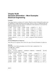
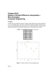
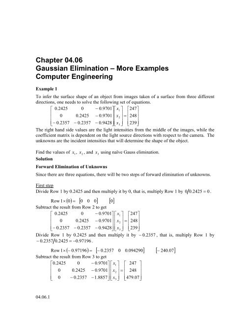
Chapter 04.06Gaussian Elimination – More ExamplesComputer EngineeringExample 1To infer the surface shape of an object from images taken of a surface from three differentdirections, one needs to solve the following set of equations.⎡ 0.2425 0 − 0.9701⎤⎡x1⎤ ⎡247⎤⎢⎥⎢⎥=⎢ ⎥⎢0 0.2425 − 0.9701⎥⎢x2⎥ ⎢248⎥⎢⎣− 0.2357 − 0.2357 − 0.9428⎥⎦⎢⎣x ⎥⎦⎢⎣239⎥3 ⎦The right hand side values are the light intensities from the middle of the images, while thecoefficient matrix is dependent on the light source directions with respect to the camera. Theunknowns are the incident intensities that will determine the shape of the object.Find the values of x1, x2, and x3using naïve Gauss elimination.SolutionForward Elimination of UnknownsSince there are three equations, there will be two steps of forward elimination of unknowns.First stepDivide Row 1 by 0.2425 and then multiply it by 0, that is, multiply Row 1 by 0 0.2425 = 0.( 0) [ 0 0 0] [ 0]Row 1×=Subtract the result from Row 2 to get⎡ 0.2425 0 − 0.9701⎤⎡x1⎤ ⎡247⎤⎢⎥ ⎢ ⎥=⎢ ⎥⎢0 0.2425 − 0.9701⎥ ⎢x2⎥ ⎢248⎥⎢⎣− 0.2357 − 0.2357 − 0.9428⎥⎦⎢⎣x ⎥⎦⎢⎣239⎥3 ⎦Divide Row 1 by 0.2425 and then multiply it by − 0. 2357 , that is, multiply Row 1 by− 0.23570.2425 = −0.97196.( − 0.97196) = [ − 0.2357 0 0.094290] [ − 240.07]Row 1×Subtract the result from Row 3 to get⎡0.24250 − 0.9701⎤⎡x1⎤ ⎡ 247 ⎤⎢⎥ ⎢ ⎥=⎢ ⎥⎢0 0.2425 − 0.9701⎥ ⎢x2⎥ ⎢248⎥⎢⎣0 − 0.2357 −1.8857⎥⎦⎢⎣x ⎥⎦⎢⎣479.07⎥3 ⎦04.06.1

04.06.2 Chapter 04.06Second stepWe now divide Row 2 by 0.2425 and then multiply by − 0. 2357 , that is, multiply Row 2 by− 0.23570.2425 = −0.97196.Row 2 × ( − 0.97196) = [ 0 − 0.2357 0.94290] [ − 241.05]Subtract the result from Row 3 to get⎡0.24250 − 0.9701⎤⎡x1⎤ ⎡ 247 ⎤⎢⎥ ⎢ ⎥=⎢ ⎥⎢0 0.2425 − 0.9701⎥ ⎢x2⎥ ⎢248⎥⎢⎣0 0 − 2.8286⎦⎥⎢⎣x ⎥⎦⎢⎣720.12⎥3 ⎦Back substitutionFrom the third equation,− 2.8286x = 3720.12720.12x3=− 2.8286= −254.59Substituting the value of x3in the second equation,0.2425x2+ ( −0.9701)x3= 248248 − ( −0.9701)x3x2=0.2425248 − ( −0.9701)× ( −254.59)=0.2425= 4.2328Substituting the values of x2and x3in the first equation,0.2425x1+ 0x2+ ( −0.9701)x3= 247247 − 0x2− ( −0.9701)x3x1=0.2425247 − ( −0.9701)× ( −254.59)=0.2425= 0.10905Hence the solution vector is⎡x1⎤ ⎡ 0.10905 ⎤⎢ ⎥=⎢ ⎥⎢x2⎥ ⎢4.2328⎥⎢⎣x ⎥⎦⎢⎣− 254.59⎥3⎦

Gaussian Elimination-More Examples: Computer Engineering 04.06.3SIMULTANEOUS LINEAR EQUATIONSTopic Gaussian Elimination – More ExamplesSummary Examples of Gaussian eliminationMajor Computer EngineeringAuthors Autar KawDate August 8, 2009Web Site http://numericalmethods.eng.usf.edu