Gaussian Elimination-More Examples: Electrical Engineering

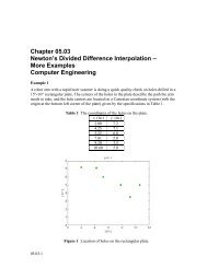
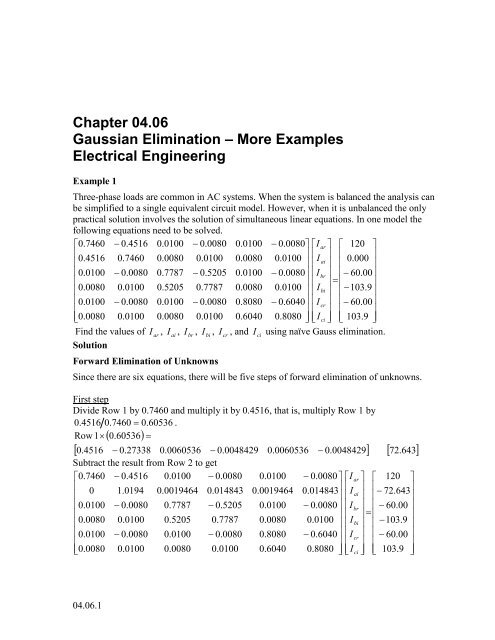
Chapter 04.06Gaussian Elimination – More ExamplesElectrical EngineeringExample 1Three-phase loads are common in AC systems. When the system is balanced the analysis canbe simplified to a single equivalent circuit model. However, when it is unbalanced the onlypractical solution involves the solution of simultaneous linear equations. In one model thefollowing equations need to be solved.⎡0.7460− 0.4516 0.0100 − 0.0080 0.0100 − 0.0080⎤⎡Iar ⎤ ⎡ 120 ⎤⎢⎥ ⎢ ⎥ ⎢ ⎥⎢0.4516 0.7460 0.0080 0.0100 0.0080 0.0100⎢I⎥ai⎥ ⎢0.000⎥⎢0.0100− 0.0080 0.7787 − 0.5205 0.0100 − 0.0080⎥⎢I⎥br⎢−60.00⎥⎢⎥ ⎢ ⎥ = ⎢ ⎥⎢0.00800.0100 0.5205 0.7787 0.0080 0.0100 ⎥ ⎢Ibi ⎥ ⎢−103.9⎥⎢0.0100− 0.0080 0.0100 − 0.0080 0.8080 − 0.6040⎥⎢I⎥ ⎢−60.00⎥cr⎢⎥ ⎢ ⎥ ⎢ ⎥⎣0.00800.0100 0.0080 0.0100 0.6040 0.8080⎦ ⎢⎣Ici ⎥⎦⎣ 103.9⎦Find the values of Iar, Iai, Ibr, Ibi, Icr, and Iciusing naïve Gauss elimination.SolutionForward Elimination of UnknownsSince there are six equations, there will be five steps of forward elimination of unknowns.First stepDivide Row 1 by 0.7460 and multiply it by 0.4516, that is, multiply Row 1 by0 .4516 0.7460 = 0.60536 .Row 1×( 0.60536)=0.4516 − 0.27338 0.0060536 − 0.0048429 0.0060536 − 0.0048429 72.643Subtract the result from Row 2 to get⎡0.7460− 0.4516 0.0100 − 0.0080 0.0100 − 0.0080⎤⎡Iar ⎤ ⎡ 120 ⎤⎢⎥ ⎢ ⎥ ⎢ ⎥⎢0 1.0194 0.0019464 0.014843 0.0019464 0.014843⎢I⎥ai⎥ ⎢− 72.643⎥⎢0.0100− 0.0080 0.7787 − 0.5205 0.0100 − 0.0080⎥⎢I⎥br⎢ − 60.00 ⎥⎢⎥ ⎢ ⎥ = ⎢ ⎥⎢0.00800.0100 0.5205 0.7787 0.0080 0.0100 ⎥ ⎢Ibi ⎥ ⎢ −103.9⎥⎢0.0100− 0.0080 0.0100 − 0.0080 0.8080 − 0.6040⎥⎢I⎥ ⎢ − 60.00 ⎥cr⎢⎥ ⎢ ⎥ ⎢ ⎥⎣0.00800.0100 0.0080 0.0100 0.6040 0.8080⎦ ⎢⎣Ici ⎥⎦⎣ 103.9⎦[ ] [ ]04.06.1

04.06.2 Chapter 04.06Divide Row 1 by 0.7460 and multiply it by 0.0100, that is, multiply Row 1 by0 .0100 0.7460 = 0.013405.Row 1×0.013405 =( )[ 0.0100 − 0.0060536 0.00013405 − 0.00010724 0.00013405 − 0.00010724] [ 1.6086]Subtract the result from Row 3 to get⎡0.7460− 0.4516 0.0100⎢⎢0 1.0194 0.0019464⎢ 0 − 0.0019464 0.77857⎢⎢0.00800.0100 0.5205⎢0.0100− 0.0080 0.0100⎢⎣0.00800.0100 0.0080− 0.00800.014843− 0.520610.7787− 0.00800.01000.01000.00194640.00986600.00800.80800.6040− 0.0080 ⎤ ⎡I0.014843⎥ ⎢⎢I⎥− 0.0078928⎥⎢I⎥ ⎢0.0100 ⎥ ⎢I− 0.6040 ⎥ ⎢I⎥ ⎢0.8080⎦ ⎢⎣Iaraibrbicrci⎤ ⎡ 120 ⎤⎥ ⎢ ⎥⎥ ⎢− 72.643⎥⎥ ⎢−61.609⎥⎥ = ⎢ ⎥⎥ ⎢ −103.9⎥⎥ ⎢ − 60.00 ⎥⎥ ⎢ ⎥⎥⎦⎣ 103.9⎦Divide Row 1 by 0.7460 and multiply it by 0.0080, that is, multiply Row 1 by0 .0080 0.7460 = 0.010724 .Row 1×( 0.010724)=−5 −50.0080 − 0.0048429 0.00010724 − 8.5791×10 0.00010724 − 8.5791×10 1.2869Subtract the result from Row 4 to get⎡0.7460− 0.4516 0.0100 − 0.0080 0.0100 − 0.0080 ⎤ ⎡Iar ⎤ ⎡ 120 ⎤⎢⎥ ⎢ ⎥ ⎢ ⎥⎢0 1.0194 0.0019464 0.014843 0.0019464 0.014843⎢I⎥ai⎥ ⎢− 72.643⎥⎢ 0 − 0.0019464 0.77857 − 0.52061 0.0098660 − 0.0078928⎥⎢I⎥br⎢−61.609⎥⎢⎥ ⎢ ⎥ = ⎢ ⎥⎢ 0 0.014843 0.52039 0.77879 0.0078928 0.010086 ⎥ ⎢Ibi ⎥ ⎢−105.19⎥⎢0.0100− 0.0080 0.0100 − 0.0080 0.8080 − 0.6040 ⎥ ⎢I⎥ ⎢ − 60.00 ⎥cr⎢⎥ ⎢ ⎥ ⎢ ⎥⎣0.00800.0100 0.0080 0.0100 0.6040 0.8080⎦ ⎢⎣Ici ⎥⎦⎣ 103.9⎦[ ] [ ]Divide Row 1 by 0.7460 and multiply it by 0.0100, that is, multiply Row 1 by0 .0100 0.7460 = 0.013405.Row 1×( 0.013405)=[ 0.0100 − 0.0060536 0.00013405 − 0.00010724 0.00013405 − 0.00010724] [ 1.6086]Subtract the result from Row 5 to get⎡0.7460− 0.4516 0.0100 − 0.0080 0.0100 − 0.0080 ⎤ ⎡Iar ⎤ ⎡ 120 ⎤⎢⎥ ⎢ ⎥ ⎢ ⎥⎢0 1.0194 0.0019464 0.014843 0.0019464 0.014843⎢I⎥ai⎥ ⎢− 72.643⎥⎢ 0 − 0.0019464 0.77857 − 0.52061 0.0098660 − 0.0078928⎥⎢I⎥br⎢−61.609⎥⎢⎥ ⎢ ⎥ = ⎢ ⎥⎢ 0 0.014843 0.52039 0.77879 0.0078928 0.010086 ⎥ ⎢Ibi ⎥ ⎢−105.19⎥⎢ 0 − 0.0019464 0.0098660 − 0.0078928 0.80787 − 0.60389 ⎥ ⎢I⎥ ⎢−61.609⎥cr⎢⎥ ⎢ ⎥ ⎢ ⎥⎣0.00800.0100 0.0080 0.0100 0.6040 0.8080⎦ ⎢⎣Ici ⎥⎦⎣ 103.9⎦Divide Row 1 by 0.7460 and multiply it by 0.0080, that is, multiply Row 1 by0 .0080 0.7460 = 0.010724 .

Gaussian Elimination-More Examples: Electrical Engineering 04.06.3Row 1×( 0.010724)=−5 −5[ 0.0080 − 0.0048429 0.00010724 − 8.5791×10 0.00010724 − 8.5791×10 ] [ 1.2869]Subtract the result from Row 6 to get⎡0.7460− 0.4516 0.0100⎢⎢0 1.0194 0.0019464⎢ 0 − 0.0019464 0.77857⎢⎢ 0 0.014843 0.52039⎢ 0 − 0.0019464 0.0098660⎢⎣ 0 0.014843 0.0078928− 0.00800.014843− 0.520390.77879− 0.00789280.0100860.01000.00194640.00986600.00789280.807870.60389− 0.0080 ⎤ ⎡I0.014843⎥ ⎢⎢I⎥− 0.0078928⎥⎢I⎥ ⎢0.010086 ⎥ ⎢I− 0.60389 ⎥ ⎢I⎥ ⎢0.80809⎦ ⎢⎣ISecond stepDivide Row 2 by 1.0194 and multiply it by −0.0019464, that is, multiply Row 2 by− 0.00194641.0194 = −0.0019094.Row 2×− 0.0019094 =( )araibrbicrci⎤ ⎡ 120 ⎤⎥ ⎢ ⎥⎥ ⎢− 72.643⎥⎥ ⎢−61.609⎥⎥ = ⎢ ⎥⎥ ⎢−105.19⎥⎥ ⎢−61.609⎥⎥ ⎢ ⎥⎥⎦⎣ 102.61⎦−6 −5−6−5[ 0 − 0.0019464 − 3.7164×10 − 2.8341×10 − 3.7164×10 − 2.8341×10 ] [ 0.13870]Subtract the result from Row 3 to get⎡0.7460− 0.4516 0.0100⎢⎢0 1.0194 0.0019464⎢ 0 0 0.77857⎢⎢ 0 0.014843 0.52039⎢ 0 − 0.0019464 0.0098660⎢⎣ 0 0.014843 0.0078928− 0.00800.014843− 0.520360.77879− 0.00789280.0100860.01000.00194640.00986970.00789280.807870.60389− 0.0080 ⎤ ⎡I0.014843⎥ ⎢⎢I⎥− 0.0078644⎥⎢I⎥ ⎢0.010086 ⎥ ⎢I− 0.60389 ⎥ ⎢I⎥ ⎢0.80809⎦ ⎢⎣Iaraibrbicrci⎤ ⎡ 120 ⎤⎥ ⎢ ⎥⎥ ⎢− 72.643⎥⎥ ⎢−61.747⎥⎥ = ⎢ ⎥⎥ ⎢−105.19⎥⎥ ⎢−61.609⎥⎥ ⎢ ⎥⎥⎦⎣ 102.61 ⎦Divide Row 2 by 1.0194 and multiply it by 0.014843, that is, multiply Row 2 by0 .014843 1.0194 = 0.014561.Row 2×( 0.014561)=− 5−5[ 0 0.014843 2.8341×10 0.00021612 2.8341×10 0.00021612] [ −1.0577]Subtract the result from Row 4 to get⎡0.7460− 0.4516 0.0100 − 0.0080 0.0100 − 0.0080 ⎤ ⎡Iar⎤ ⎡ 120 ⎤⎢⎥ ⎢ ⎥ ⎢ ⎥⎢0 1.0194 0.0019464 0.014843 0.0019464 0.014843⎢I⎥ai⎥ ⎢− 72.643⎥⎢ 0 0 0.77857 − 0.52036 0.0098697 − 0.0078644⎥⎢I⎥br⎢−61.747⎥⎢⎥ ⎢ ⎥ = ⎢ ⎥⎢ 0 0 0.52036 0.77857 0.0078644 0.0098697 ⎥ ⎢Ibi⎥ ⎢−104.13⎥⎢ 0 − 0.0019464 0.0098660 − 0.0078928 0.80787 − 0.60389 ⎥ ⎢I⎥ ⎢−61.609⎥cr⎢⎥ ⎢ ⎥ ⎢ ⎥⎣ 0 0.014843 0.0078928 0.010086 0.60389 0.80809⎦ ⎢⎣Ici⎥⎦⎣ 102.61⎦Divide Row 2 by 1.0194 and multiply it by −0.0019464, that is, multiply Row 2 by− 0.00194641.0194 = −0.0019094.

04.06.4 Chapter 04.06Row 2×( − 0.0019094)=−6 −5−6−5[ 0 − 0.0019464 − 3.7164×10 − 2.8341×10 − 3.7164×10 − 2.8341×10 ] [ 0.13870]Subtract the result from Row 5 to get⎡0.7460− 0.4516 0.0100 − 0.0080⎢⎢0 1.0194 0.0019464 0.014843⎢ 0 0 0.77857 − 0.52036⎢⎢ 0 0 0.52036 0.77857⎢ 0 0 0.0098697 − 0.0078644⎢⎣ 0 0.014843 0.0078928 0.0100860.01000.00194640.00986970.00786440.807870.60389− 0.0080 ⎤ ⎡I0.014843⎥ ⎢⎢I⎥− 0.0078644⎥⎢I⎥ ⎢0.0098697 ⎥ ⎢I− 0.60386 ⎥ ⎢I⎥ ⎢0.80809⎦ ⎢⎣Iaraibrbicrci⎤ ⎡ 120 ⎤⎥ ⎢ ⎥⎥ ⎢− 72.643⎥⎥ ⎢−61.747⎥⎥ = ⎢ ⎥⎥ ⎢−104.13⎥⎥ ⎢−61.747⎥⎥ ⎢ ⎥⎥⎦⎣ 102.61⎦Divide Row 2 by 1.0194 and multiply it by 0.014843, that is, multiply Row 2 by0 .014843 1.0194 = 0.014561.Row 2×( 0.014561)=− 5−5[ 0 0.014843 2.8341×10 0.00021612 2.8341×10 0.00021612] [ −1.0577]Subtract the result from Row 6 to get⎡0.7460− 0.4516 0.0100 − 0.0080 0.0100 − 0.0080 ⎤ ⎡Iar⎤ ⎡ 120 ⎤⎢⎥ ⎢ ⎥ ⎢ ⎥⎢0 1.0194 0.0019464 0.014843 0.0019464 0.014843⎢I⎥ai⎥ ⎢− 72.643⎥⎢ 0 0 0.77857 − 0.52036 0.0098697 − 0.0078644⎥⎢I⎥br⎢−61.747⎥⎢⎥ ⎢ ⎥ = ⎢ ⎥⎢ 0 0 0.52036 0.77857 0.0078644 0.0098697 ⎥ ⎢Ibi⎥ ⎢−104.13⎥⎢ 0 0 0.0098697 − 0.0078644 0.80787 − 0.60386 ⎥ ⎢I⎥ ⎢−61.747⎥cr⎢⎥ ⎢ ⎥ ⎢ ⎥⎣ 0 0 0.0078644 0.0098697 0.60386 0.80787⎦ ⎢⎣Ici⎥⎦⎣ 103.67⎦Third stepDivide Row 3 by 0.77857 and multiply it by 0.52036, that is, multiply Row 3 by0 .52036 0.77857 = 0.66836 .Row 3×( 0.66836)=[ 0 0 0.52036 − 0.34779 0.0065965 − 0.0052563] [ − 41.269]Subtract the result from Row 4 to get⎡0.7460− 0.4516 0.0100 − 0.0080 0.0100 − 0.0080 ⎤ ⎡Iar⎤ ⎡ 120 ⎤⎢⎥ ⎢ ⎥ ⎢ ⎥⎢0 1.0194 0.0019464 0.014843 0.0019464 0.014843⎢I⎥ai⎥ ⎢− 72.643⎥⎢ 0 0 0.77857 − 0.52036 0.0098697 − 0.0078644⎥⎢I⎥br⎢−61.747⎥⎢⎥ ⎢ ⎥ = ⎢ ⎥⎢ 0 0 0 1.1264 0.0012679 0.015126 ⎥ ⎢Ibi⎥ ⎢−62.860⎥⎢ 0 0 0.0098697 − 0.0078644 0.80787 − 0.60386 ⎥ ⎢I⎥ ⎢−61.747⎥cr⎢⎥ ⎢ ⎥ ⎢ ⎥⎣ 0 0 0.0078644 0.0098697 0.60386 0.80787⎦ ⎢⎣Ici⎥⎦⎣ 103.67⎦Divide Row 3 by 0.77857 and multiply it by 0.0098697, that is, multiply Row 3 by0 .0098697 0.77857 = 0.012677 .

Gaussian Elimination-More Examples: Electrical Engineering 04.06.5Row 3×( 0.012677)=− 5[ 0 0 0.0098697 − 0.0065965 0.00012511 − 9.9695×10 ] [ − 0.78275]Subtract the result from Row 5 to get⎡0.7460− 0.4516 0.0100 − 0.0080⎢⎢0 1.0194 0.0019464 0.014843⎢ 0 0 0.77857 − 0.52036⎢⎢ 0 0 0 1.1264⎢ 0 0 0 − 0.0012679⎢⎣ 0 0 0.0078644 0.00986970.01000.00194640.00986970.00126790.807740.60386− 0.0080 ⎤ ⎡I0.014843⎥ ⎢⎢I⎥− 0.0078644⎥⎢I⎥ ⎢0.015126 ⎥ ⎢I− 0.60376 ⎥ ⎢I⎥ ⎢0.80787⎦ ⎢⎣Iaraibrbicrci⎤ ⎡ 120 ⎤⎥ ⎢ ⎥⎥ ⎢− 72.643⎥⎥ ⎢−61.747⎥⎥ = ⎢ ⎥⎥ ⎢−62.860⎥⎥ ⎢−60.965⎥⎥ ⎢ ⎥⎥⎦⎣ 103.67⎦Divide Row 3 by 0.77857 and multiply it by 0.0078644, that is, multiply Row 3 by0 .0078644 0.77857 = 0.010101.Row 3×( 0.010101)=− 5−5[ 0 0 0.0078644 − 0.0052563 9.9695×10 − 7.9439×10 ] [ − 0.62372]Subtract the result from Row 6 to get⎡0.7460− 0.4516 0.0100 − 0.0080 0.0100 − 0.0080 ⎤ ⎡Iar⎤ ⎡ 120 ⎤⎢⎥ ⎢ ⎥ ⎢ ⎥⎢0 1.0194 0.0019464 0.014843 0.0019464 0.014843⎢I⎥ai⎥ ⎢− 72.643⎥⎢ 0 0 0.77857 − 0.52036 0.0098697 − 0.0078644⎥⎢I⎥br⎢−61.747⎥⎢⎥ ⎢ ⎥ = ⎢ ⎥⎢ 0 0 0 1.1264 0.0012679 0.015126 ⎥ ⎢Ibi⎥ ⎢−62.860⎥⎢ 0 0 0 − 0.0012679 0.80774 − 0.60376 ⎥ ⎢I⎥ ⎢−60.965⎥cr⎢⎥ ⎢ ⎥ ⎢ ⎥⎣ 0 0 0 0.015126 0.60376 0.80795⎦ ⎢⎣Ici⎥⎦⎣ 104.29⎦Fourth stepDivide Row 4 by 1.1264 and multiply it by −0.0012679, that is, multiply Row 4 by− 0.00126791.1264 = −0.0011257.Row 4×( − 0.0011257)=−6 −5[ 0 0 0 − 0.0012679 −1.4273×10 −1.7027× 10 ] [ 0.070761]Subtract the result from Row 5 to get⎡0.7460− 0.4516 0.0100 − 0.0080 0.0100 − 0.0080 ⎤ ⎡Iar⎤ ⎡ 120 ⎤⎢⎥ ⎢ ⎥ ⎢ ⎥⎢0 1.0194 0.0019464 0.014843 0.0019464 0.014843⎢I⎥ai⎥ ⎢− 72.643⎥⎢ 0 0 0.77857 − 0.52036 0.0098697 − 0.0078644⎥⎢I⎥br⎢−61.747⎥⎢⎥ ⎢ ⎥ = ⎢ ⎥⎢ 0 0 0 1.1264 0.0012679 0.015126 ⎥ ⎢Ibi⎥ ⎢−62.860⎥⎢ 0 0 0 0 0.80775 − 0.60375 ⎥ ⎢I⎥ ⎢−61.035⎥cr⎢⎥ ⎢ ⎥ ⎢ ⎥⎣ 0 0 0 0.015126 0.60376 0.80795⎦ ⎢⎣Ici⎥⎦⎣ 104.29⎦Divide Row 4 by 1.1264 and multiply it by 0.015126, that is, multiply Row 4 by0 .015126 1.1264 = 0.013429 .

04.06.6 Chapter 04.06Row 4 ×( 0.013429)=− 5[ 0 0 0 0.015126 1.7027 × 10 0.00020313] [ − 0.84415]Subtract the result from Row 6 to get⎡0.7460− 0.4516 0.0100 − 0.0080⎢0 1.0194 0.0019464 0.014843⎢⎢ 0 0 0.77857 − 0.52036⎢⎢0 0 0 1.1264⎢ 0 0 0 0⎢⎣ 0 0 0 00.01000.00194640.00986970.00126790.807750.60375− 0.0080 ⎤ ⎡I0.014843⎥ ⎢I⎥ ⎢− 0.0078644⎥⎢I⎥ ⎢0.015126⎥ ⎢I− 0.60375 ⎥ ⎢I⎥ ⎢0.80775 ⎦ ⎣IFifth stepDivide Row 5 by 0.80775 and multiply it by 0.60375, that is, multiply Row 5 by0 .60375 0.80775 = 0.74745.Row 5×0.74741 =( )[ 0 0 0 0 0.60375 − 0.45127] [ − 45.621]Subtract the result from Row 6 to get⎡0.7460− 0.4516 0.0100 − 0.0080⎢0 1.0194 0.0019464 0.014843⎢⎢ 0 0 0.77857 − 0.52036⎢⎢0 0 0 1.1264⎢ 0 0 0 0⎢⎣ 0 0 0 00.01000.00194640.00986970.00126790.807750− 0.0080 ⎤ ⎡I0.014843⎥ ⎢I⎥ ⎢− 0.0078644⎥⎢I⎥ ⎢0.015126⎥ ⎢I− 0.60375 ⎥ ⎢I⎥ ⎢1.2590 ⎦ ⎣IThe six equations are0 .7460 Iar+ − 0.4516 Iai+ 0.0100Ibr+ − 0.0080 Ibi+ 0.0100Icr+ − 0.0080 Ici=1.0194Iai+ 0.0019464 Ibr+ 0.014843Ibi+ 0.0019464 Icr+ 0.014843Ici= −72.6430.77857Ibr− 0.52036Ibi+ 0.0098697 Icr+ ( − 0.0078644) Ici= −61.7471.1264Ibi+ 0.0012679 Icr+ 0.015126 Ici= −62.8600.80775Icr+ ( −0.60375)Ici= −61.0351 .2590 Ici= 150.75Back SubstitutionFrom the sixth equation1 .2590 Ici= 150.75150.75Ici=1.2590= 119.74Substituting the value of Iciin the fifth equation,.80775I+ ( −0.60375)I= −61.035araibrbicrciaraibrbicrci⎤ ⎡ 120 ⎤⎥ ⎢− 72.643⎥⎥ ⎢ ⎥⎥ ⎢−61.747⎥⎥ = ⎢ ⎥⎥ ⎢− 62.860⎥⎥ ⎢−61.035⎥⎥ ⎢ ⎥⎦ ⎣ 105.13 ⎦⎤ ⎡ 120 ⎤⎥ ⎢− 72.643⎥⎥ ⎢ ⎥⎥ ⎢−61.747⎥⎥ = ⎢ ⎥⎥ ⎢− 62.860⎥⎥ ⎢−61.035⎥⎥ ⎢ ⎥⎦ ⎣ 150.75 ⎦( ) ( ) ( ) 1200crci

Gaussian Elimination-More Examples: Electrical Engineering 04.06.7− 61.035− ( −0.60375)IciIcr=0.80775= 13.938Substituting the value of Icrand Iciin the forth equation,1.1264I0.0012679 I + 0.015126 I = −62.860bi+crci62.860− 0.0012679 Icr− 0.015126 Ici−Ibi=1.1264= −57.429Substituting the value of Ibi, Icrand Iciin the third equation,0 77857 I − 0.52036I+ 0.0098697 I + − 0.0078644 I = −61.( ) 747.brbicrci− 61.747+ 0.52036Ibi− 0.0098697 Icr− ( −0.0078644)Icibr=I0.77857= −116.66Substituting the value of Ibr, Ibi, Icrand Iciin the second equation,1.0194I 0.0019464 I + 0.014843I+ 0.0019464 I + 0.014843I= −72.643ai+brbicrci72.643− 0.0019464 Ibr− 0.014843Ibi− 0.0019464 Icr− 0.014843Ici−Iai=1.0194= −71.972Substituting the value of Iai, Ibr, Ibi, Icr, and Iciin the first equation,0 .7460 I ( −0.4516)I + 0.0100I+ ( −0.0080)I + 0.0100I+ ( −0.0080)I = 120ar+aibrbicrci120 − ( −0.4516)Iai− 0.0100Ibr− ( −0.0080)Ibi− 0.0100Icr− ( −0.0080)IciIar=0.7460= 119.33Hence the solution vector is⎡Iar ⎤ ⎡ 119.33 ⎤⎢I⎥ ⎢−⎥⎢ai71.972⎥ ⎢ ⎥⎢Ibr⎥ ⎢−116.66⎥⎢ ⎥ = ⎢ ⎥⎢Ibi ⎥ ⎢− 57.429⎥⎢I⎥ ⎢ 13.938 ⎥cr⎢ ⎥ ⎢ ⎥⎣Ici ⎦ ⎣ 119.74 ⎦SIMULTANEOUS LINEAR EQUATIONSTopic Gaussian Elimination – More ExamplesSummary Examples of Gaussian eliminationMajor Electrical EngineeringAuthors Autar KawDate June 15, 2010Web Site http://numericalmethods.eng.usf.edu