Modeling and Inversion in Thermal Infrared Remote Sensing over ...

More documents

Recommendations

Info

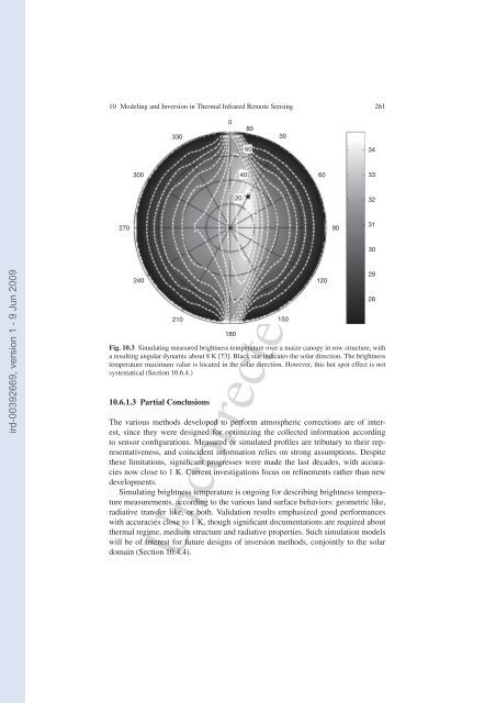
260 F. Jacob et al.ird-00392669, version 1 - 9 Jun 2009content as a polynomial of MODIS near infrared radiance ratios, with a 0.4 g. cm −2accuracy. Atmospheric sounders allow inferring profiles of temperature and watervapor density, using Eq. 10.6 or neural networks [3, 4]. Previous sounders such asTOVS permitted to reach a 0.4 g. cm −2 accuracy on water vapor content [200]. Newsounders such as IASI [201], with finer spectral samplings and spatial resolutions,should provide accuracies better than 1 K and 10% for atmospheric profiles of temperatureand humidity.10.6.1.2 Land Surface Radiative Regime and Related MeasurementsSurface brightness temperature is simulated using simple radiative transfer equationsor simulation models. The former provide easy and efficient solutions for assimilatingTIR remote sensing data into land process models. The latter are fine andaccurate solutions for understanding well TIR remotely sensed measurements.To constrain land process model parameters, surface brightness temperature canbe simulated using simple radiative transfer equations coupled with SVAT models.[39] coupled the composite surface radiative transfer equation (Eq. 10.7) witha crop and a one source SVAT model. The latter calculated ensemble radiometrictemperature by closing surface energy budget. R-emissivity was estimated usingthe SAIL TIR version of [136], documented by the crop model for vegetationstructural parameters. Similarly, [67] coupled the soil and vegetation radiative transferequation (Eq. 10.10) with a two source SVAT model. The latter calculated soiland vegetation temperatures by closing energy budget for each, while setting soiland vegetation emissivities to nominal values.Calculating surface brightness temperature from simulation models requires informationabout vegetation structure (row crop, LAI, LIDF, cover fraction), soiland vegetation radiative properties (emissivity, reflectance), and thermal regime(canopy temperature distribution). The latter can be derived from a SVAT model,which solves local energy budget according to meteorological conditions (solarposition, wind speed, air temperature), vegetation status (leaf stomatal resistance),and soil moisture. Then, simulation models mimic the radiative regime using moreor less complex descriptions of the thermal regime: a unique vegetation temperature[73], soil and vegetation temperatures with optional sunlit and shaded components[74, 137], additional vegetation layer temperatures for specific crops [145], orcanopy temperature profile [78].Simulation models are currently under development, verification and analysis[73, 74, 76, 78, 144, 145]. Current investigations focus on spectral behaviors [120],but especially on directional effects which allow normalizing multiangular observations(Fig. 10.3). For instance, [58, 72] angularly normalized water stress indicesover row structured crops. Similarly, [202] normalized across track observationsfrom sun-view geometry effects, for a daily monitoring at the continental scale.Uncorrected Proof
10 Modeling and Inversion in Thermal Infrared Remote Sensing 261ird-00392669, version 1 - 9 Jun 2009270300240330210018020408060Fig. 10.3 Simulating measured brightness temperature over a maize canopy in row structure, witha resulting angular dynamic about 8 K [73]. Black star indicates the solar direction. The brightnesstemperature maximum value is located in the solar direction. However, this hot spot effect is notsystematical (Section 10.6.4.)10.6.1.3 Partial ConclusionsThe various methods developed to perform atmospheric corrections are of interest,since they were designed for optimizing the collected information accordingto sensor configurations. Measured or simulated profiles are tributary to their representativeness,and coincident information relies on strong assumptions. Despitethese limitations, significant progresses were made the last decades, with accuraciesnow close to 1 K. Current investigations focus on refinements rather than newdevelopments.Simulating brightness temperature is ongoing for describing brightness temperaturemeasurements, according to the various land surface behaviors: geometric like,radiative transfer like, or both. Validation results emphasized good performanceswith accuracies close to 1 K, though significant documentations are required aboutthermal regime, medium structure and radiative properties. Such simulation modelswill be of interest for future designs of inversion methods, conjointly to the solardomain (Section 10.4.4).150120Uncorrected Proof30609034333231302928
Page 1: Author manuscript, published in "Ad
Page 4 and 5: 246 F. Jacob et al.ird-00392669, ve
Page 7 and 8: 10 Modeling and Inversion in Therma
Page 9: 10 Modeling and Inversion in Therma
Page 17: 10 Modeling and Inversion in Therma
Page 53 and 54: Glossaryird-00392669, version 1 - 9

Modeling and Inversion in Thermal Infrared Remote Sensing over ...

You also want an ePaper? Increase the reach of your titles

Delete template?

Save as template?