Modeling and Inversion in Thermal Infrared Remote Sensing over ...

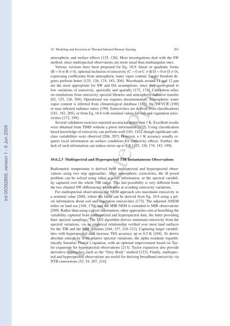
10 Modeling and Inversion in Thermal Infrared Remote Sensing 263ird-00392669, version 1 - 9 Jun 2009atmospheric and surface effects [125, 126]. Most investigations deal with the SWmethod, since multispectral observations are more usual than multiangular ones.Various versions have been proposed for Eq. 10.9: linear or quadratic forms(B = 0orB≠ 0), optional inclusion of emissivity (C = 0orC≠ 0, D = 0orD≠ 0),expressing coefficients from atmospheric water vapor content. Larger freedom degreesperform better [125, 126, 174, 183, 204]. Wavebands around 11 and 12 µmare the most appropriate for SW and DA assumptions, since they correspond tolow variations of emissivity, spectrally and spatially [172, 174]. Calibration relieson simulations from emissivity spectral libraries and atmospheric radiative transfer[82, 125, 126, 204]. Operational use requires documentation. Atmospheric watervapor content is inferred from climatological database [183], the SWVCR [198]or near infrared radiance ratios [199]. Emissivities are derived from classifications[181, 182, 205], or from Eq. 10.8 with nominal values for soil and vegetation emissivities[172, 199].Several validation exercises reported accuracies better than 1 K. Excellent resultswere obtained from TIMS without a priori information [172]. Using classificationbased knowledge of emissivity can perform well [181, 182], though significant subclassvariabilities were observed [206, 207]. However, a 1 K accuracy usually requireslocal information on surface conditions for emissivity effects. Further, thelack of such information can induce errors up to 3 K [125, 126, 174, 183, 199].10.6.2.3 Multispectral and Hyperspectral TIR Instantaneous ObservationsRadiometric temperature is derived from multispectral and hyperspectral observationsusing two step approaches. After atmospheric corrections, the ill posedproblem can be solved using either a priori information, or the spectral variabilitycaptured over the whole TIR range. This last possibility is very different fromthe two channel SW differencing which aims at avoiding emissivity variations.For multispectral observations, the NEM approach sets maximum emissivity toa nominal value [208], where the latter can be derived from Eq. 10.8 using a prioriinformation about soil and vegetation emissivities [173]. The adjusted ANEMrelies on land use [168, 170], and the MIR NEM is extended to MIR observations[209]. Rather than using a priori information, other approaches aim at benefiting thevariability captured from multispectral and hyperspectral data, the latter providingfiner spectral samplings. The TES algorithm derives minimum emissivity from thespectral variations, via an empirical relationship verified over most land surfacesfor the TIR and the MIR domains [104, 157, 210–212]. Capturing larger variabilitieswith hyperspectral data increase TES accuracy up to 0.5 K [104]. To deriveabsolute emissivity from relative spectral variations, the alpha residuals logarithmicallylinearize Planck’s equation, with an optional improvement based on Taylorexpansion for hyperspectral observations [213]. Taylor expansion also providederivative approaches, such as the “Grey Body” method [123]. Finally, multispectraland hyperspectral observations are useful for deriving broadband emissivity viaNTB conversions [52, 54, 207, 214].Uncorrected Proof